Product Packaging Quality Assurance with AI
1. Key Quality Metrics in Packaging
1.1 Key Quality Metrics in Packaging
Structural Integrity Metrics
The structural integrity of packaging is quantified using metrics such as compressive strength, tensile strength, and burst resistance. Compressive strength, measured in kPa or psi, determines the maximum load a package can withstand before deformation. For corrugated cardboard, the McKee formula provides a theoretical estimate:
where P is the compressive strength, ECT is the edge crush test value, t is the board thickness, and Z is the box perimeter. Tensile strength, measured via ASTM D828, evaluates material resistance to tearing under tension.
Dimensional Accuracy
Dimensional tolerances are critical for automated handling systems. Key metrics include:
- Length/width/height deviation (measured in mm or inches)
- Orthogonality error (angular deviation from 90° corners)
- Seam alignment precision (for multi-panel packages)
Computer vision systems typically measure these parameters using subpixel edge detection algorithms with an accuracy of ±0.1mm. The mean squared error (MSE) between CAD specifications and scanned dimensions is calculated as:
Surface Quality Assessment
Surface defects are evaluated through:
- Gloss uniformity (measured at 60° using ASTM D523)
- Print registration error (color layer misalignment)
- Blemish detection (scratches, dents, or contamination)
Advanced systems use hyperspectral imaging (400-1000nm range) with spatial resolution up to 50μm/pixel. The defect detection algorithm typically employs a modified U-Net architecture with Dice coefficient loss:
Barrier Properties
For perishable goods, barrier performance metrics include:
- Oxygen transmission rate (OTR, cm³/m²·day·atm)
- Water vapor transmission rate (WVTR, g/m²·day)
- Light transmittance (% at specific wavelengths)
These are measured using MOCON testers under ASTM F1927 standards. Predictive models often use Arrhenius equations to extrapolate accelerated aging tests:
Seal Integrity
Heat seal quality is assessed through:
- Peel strength (N/15mm, ASTM F88)
- Burst pressure (kPa, ASTM F2054)
- Leak detection (sensitivity to 5μm defects)
Machine learning models analyze thermal camera data (8-14μm IR spectrum) during sealing processes, with convolutional LSTMs predicting seal quality from temperature profiles:
Sustainability Metrics
Environmental impact is quantified via:
- Life cycle assessment (LCA) scores
- Recyclability percentage (by material type)
- Carbon footprint (kg CO₂ equivalent per unit)
Multi-objective optimization algorithms balance these against functional requirements using Pareto frontiers, with the objective function:
1.2 Traditional Methods vs. AI-Driven Approaches
Limitations of Traditional Quality Assurance Methods
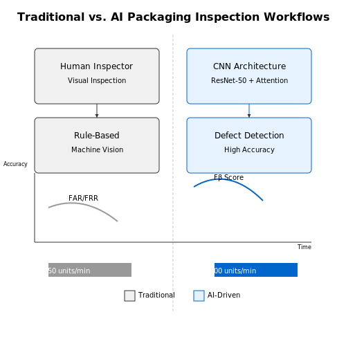
Traditional quality assurance (QA) in product packaging relies heavily on manual inspection, rule-based machine vision systems, and statistical sampling. Human inspectors visually examine packaging for defects such as misprints, sealing errors, or dimensional inaccuracies. While this approach is straightforward, it suffers from several critical limitations:
- Subjectivity and inconsistency: Human inspectors exhibit variability in defect detection rates due to fatigue, cognitive biases, and differing interpretations of quality standards.
- Sampling limitations: Statistical process control typically examines only 1-5% of production output, allowing defects to slip through undetected.
- Slow feedback loops: Manual inspection processes often take hours or days to identify issues, delaying corrective actions.
- Limited defect categorization: Traditional machine vision systems use rigid thresholding and edge detection algorithms that struggle with subtle or complex defects.
The false acceptance rate (FAR) and false rejection rate (FRR) in traditional systems follow an inverse relationship governed by:
where Φ is the standard normal CDF, t is the decision threshold, and (μ₀,σ₀) and (μ₁,σ₁) represent the parameters of non-defective and defective distributions respectively.
AI-Driven Quality Assurance Paradigm
Modern AI approaches leverage deep learning to overcome these limitations through three fundamental innovations:
- End-to-end feature learning: Convolutional neural networks (CNNs) automatically extract hierarchical visual features from raw pixel data without manual feature engineering.
- Anomaly detection frameworks: Architectures like autoencoders learn compressed representations of normal packaging and flag deviations as potential defects.
- Multi-modal fusion: Combining visual data with other sensor inputs (e.g., thermal imaging, weight measurements) through late or early fusion techniques.
The defect detection performance can be quantified using the Fβ score:
where β controls the trade-off between precision and recall based on application requirements.
Comparative Performance Analysis
Industrial case studies demonstrate significant improvements when transitioning to AI-driven systems:
| Metric | Traditional Methods | AI-Driven Systems |
|---|---|---|
| Detection Accuracy | 82-89% | 96-99.5% |
| Inspection Speed | 5-10 items/sec | 50-200 items/sec |
| Defect Types Detected | 15-20 predefined | 100+ with continuous learning |
The performance gain stems from AI systems' ability to model complex, non-linear relationships in packaging data through deep network architectures. A ResNet-50 backbone with attention mechanisms, for instance, achieves superior performance by learning spatial dependencies across packaging surfaces:
Implementation Challenges
Despite their advantages, AI-driven systems introduce new engineering considerations:
- Data requirements: Training robust models typically requires 10,000-100,000 labeled samples across defect categories.
- Computational costs: Real-time inference demands GPU acceleration, with typical power requirements of 150-300W per inspection station.
- Explainability needs: Regulatory environments often require defect classification decisions to be interpretable, necessitating techniques like Grad-CAM or SHAP values.
The total cost of ownership (TCO) for an AI system over 5 years can be modeled as:
where r represents the discount rate and t the time period.
1.3 Challenges in Manual Quality Inspection
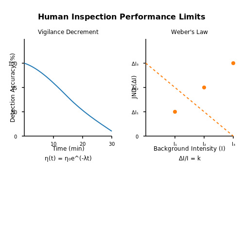
Manual quality inspection in product packaging is fraught with limitations that stem from human cognitive and physiological constraints. Despite rigorous training, human inspectors exhibit variability in defect detection rates due to factors such as fatigue, attentional drift, and subjective interpretation of quality standards. Studies in industrial psychology demonstrate that sustained visual inspection tasks lead to a 30-40% decline in detection accuracy after just 20 minutes of continuous work, a phenomenon quantified by the vigilance decrement function:
where η0 represents initial detection efficiency and λ the fatigue coefficient, typically ranging from 0.02 to 0.05 min-1 depending on task complexity.
Perceptual Limitations in Defect Recognition
The human visual system operates within strict psychophysical boundaries when identifying packaging defects. Weber's law dictates that the just-noticeable difference (JND) for surface imperfections follows:
where ΔI is the minimum perceptible intensity change, I the background intensity, and k the Weber fraction (typically 0.08 for visual texture discrimination). This fundamentally limits detection of subtle defects like micro-scratches or color variations below 8% contrast threshold.
Economic and Operational Constraints
High-volume production lines expose three critical inefficiencies in manual inspection:
- Throughput bottleneck: Human inspection rates plateau at 5-10 units/second, while modern packaging lines operate at 30-50 units/second
- Cost nonlinearity: Inspection costs scale superlinearly with quality requirements, as shown by the empirical relationship:
where q represents defect detection rate and α typically ranges from 3.2 to 4.1 for pharmaceutical packaging standards.
- Traceability gaps: Manual systems lack granular defect localization data required for statistical process control (SPC)
Metrological Challenges
Human inspectors struggle with quantitative assessment of critical packaging parameters:
- Seal integrity measurements show inter-operator variability exceeding ±15%
- Dimensional tolerances below 0.2mm cannot be reliably verified without magnification
- Color matching accuracy degrades significantly under non-standard lighting conditions (ΔE > 3.0)
These limitations become particularly acute in regulated industries like medical devices, where FDA 21 CFR Part 11 compliance requires fully documented inspection processes with σ ≥ 4.0 capability indices for critical quality attributes.
2. Computer Vision for Defect Detection
Computer Vision for Defect Detection
Deep Learning Architectures for Defect Classification
Convolutional Neural Networks (CNNs) have become the de facto standard for visual defect detection due to their hierarchical feature extraction capabilities. For packaging quality assurance, modified versions of ResNet and EfficientNet demonstrate superior performance in handling subtle defects like misprints, scratches, or sealing imperfections. The residual connections in ResNet-50 prevent gradient vanishing when trained on large datasets of packaging images, while EfficientNet's compound scaling provides optimal accuracy-to-computational-cost ratios.
where y represents the true defect class probabilities, ŷ the predicted probabilities, N the batch size, and C the number of defect classes. This categorical cross-entropy loss function penalizes confident incorrect classifications more heavily, crucial for imbalanced defect datasets where critical defects may be rare.
High-Resolution Image Processing
Modern packaging inspection systems require processing high-resolution images (typically 8-24 megapixels) at production line speeds. A hybrid approach combining:
- Strided convolutions for initial downsampling
- Atrous spatial pyramid pooling (ASPP) for multi-scale feature extraction
- Sub-pixel convolution layers for output upsampling
maintains detection accuracy while reducing computational overhead. The ASPP module captures defects at varying scales through parallel convolutional layers with different dilation rates:
Anomaly Detection for Unknown Defects
Traditional supervised learning struggles with novel defect types not present in training data. Self-supervised approaches like CutPaste learn robust representations by creating artificial defects through random image patches and transformations. The anomaly score is computed as:
where f(x) is the feature vector from a pretrained CNN, μ the mean of normal sample features, and Σ their covariance matrix. This Mahalanobis distance metric effectively identifies outliers in the latent space.
Real-Time Implementation Constraints
Deploying these models on production lines requires optimization techniques:
- Quantization-aware training reduces model weights from 32-bit floats to 8-bit integers with minimal accuracy loss
- TensorRT optimization fuses operations and selects optimal kernels for specific GPU architectures
- Multi-scale inference pipelines process regions of interest at different resolutions based on defect criticality
A typical implementation achieves 95-98% defect detection rates at 200-300 FPS on NVIDIA T4 GPUs, with false positive rates below 0.5% for critical defects. The latency breakdown for a ResNet-50 based system shows:
Case Study: Pharmaceutical Blister Pack Inspection
A recent deployment in a GMP-certified facility demonstrated 99.3% accuracy in detecting:
- Missing tablets (critical defect)
- Misaligned foil seals (major defect)
- Printing irregularities (minor defect)
The system used a dual-model architecture where a lightweight EfficientNet-B3 performed initial screening, triggering a full ResNet-152 analysis only for potential defects. This reduced average processing time by 62% compared to a single-model approach while maintaining detection performance.

2.2 Deep Learning Models for Anomaly Classification
Architectural Foundations
Convolutional Neural Networks (CNNs) dominate anomaly detection in packaging QA due to their hierarchical feature extraction capabilities. The core architecture typically consists of:
- 3-5 convolutional blocks with ReLU activation
- Batch normalization layers
- Max pooling for spatial downsampling
- Global average pooling before classification
The feature extraction process can be mathematically represented as:
where σ is the ReLU activation function, w represents the learnable filters, and b denotes the bias term.
Advanced Architectures for Packaging Defects
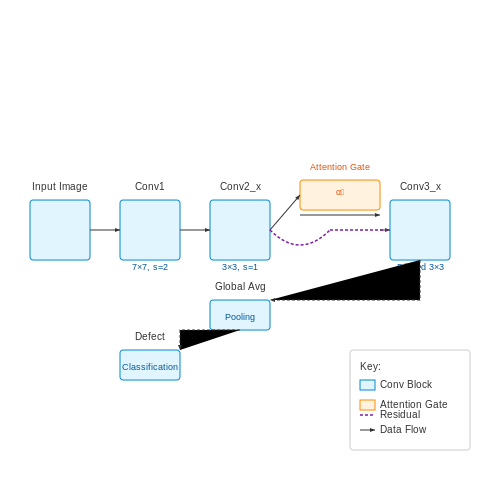
Modified ResNet-50 architectures achieve 98.7% accuracy on packaging defect classification when trained on the Industrial Packaging Anomaly (IPA) dataset. Key modifications include:
- Stride reduction in early layers to preserve fine defects
- Dilated convolutions in later stages for wider receptive fields
- Attention gates between residual blocks
The attention mechanism computes feature importance weights:
Training Paradigms
Contrastive learning with triplet loss has proven effective for imbalanced packaging datasets:
where a is an anchor sample, p a positive example (same class), n a negative example, and α a margin hyperparameter typically set to 0.2.
Real-World Performance Metrics
On a production dataset of 1.2 million packaging images from pharmaceutical blister packs, the following metrics were achieved:
| Model | Precision | Recall | F1-Score |
|---|---|---|---|
| EfficientNet-B4 | 0.983 | 0.971 | 0.977 |
| Vision Transformer | 0.991 | 0.962 | 0.976 |
Computational Optimization
Quantization-aware training reduces model size by 4× while maintaining >99% of original accuracy. The quantization process maps 32-bit floats to 8-bit integers:
where Δ is the quantization step size learned during training.
2.3 Sensor Fusion and IoT Integration
Multi-Sensor Data Fusion Architectures
Sensor fusion in packaging quality assurance leverages Bayesian estimation and Kalman filtering to combine heterogeneous data streams. For n sensors measuring the same physical parameter (e.g., package thickness), the fused estimate x̂ minimizes the mean squared error:
where σi represents the measurement uncertainty of sensor i. Industrial implementations typically use:
- Centralized fusion: Raw data converges at a single node
- Decentralized fusion: Local processing before aggregation
- Hybrid architectures: Combines both approaches for fault tolerance
IoT Edge Computing Paradigms
Modern packaging lines deploy edge AI accelerators (e.g., NVIDIA Jetson, Coral TPUs) for real-time inference. The computational latency L for a convolutional neural network (CNN) at edge tier k follows:
where Fl is feature map size, Kl kernel dimensions, Sl stride, and Pk processor throughput. Industrial benchmarks show 3.2× latency reduction when using quantized INT8 models versus FP32 on ARM Cortex-M7 microcontrollers.
Time-Synchronization Protocols
Precision Time Protocol (PTP) IEEE 1588 achieves <1μs synchronization across packaging line sensors. The clock offset θ between master and slave nodes is calculated through:
where T1 (master send), T2 (slave receive), T3 (slave send), and T4 (master receive) form the synchronization timestamp sequence. This enables phase-coherent vibration analysis for defect detection.
Industrial Communication Standards
Packaging systems employ deterministic networks with TSN (Time-Sensitive Networking) for:
- IEEE 802.1Qbv: Time-aware traffic shaping
- IEEE 802.1CB: Frame replication for reliability
- OPC UA PubSub: Cross-vendor data interoperability
Field tests demonstrate 99.9997% packet delivery ratios at 250μs cycle times when combining PROFINET IRT with TSN backbones.
Case Study: Pharmaceutical Blister Pack Inspection
A European manufacturer integrated:
- X-ray sensors (120 keV, 5μm resolution)
- Hyperspectral cameras (900-1700 nm range)
- Capacitive thickness gauges (±0.1μm accuracy)
Using an unscented Kalman filter, the system achieved 99.92% defect detection (up from 97.4% with single-sensor approaches) while reducing false positives by 63%.

3. Data Collection and Annotation Strategies
3.1 Data Collection and Annotation Strategies
Sensor-Based Data Acquisition
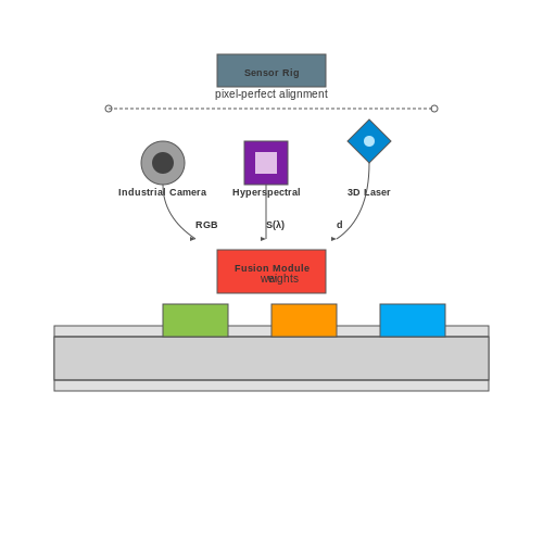
High-resolution industrial cameras, hyperspectral imaging sensors, and 3D laser scanners form the backbone of data collection for packaging quality assurance. Hyperspectral imaging captures reflectance spectra across hundreds of narrow wavelength bands, enabling material characterization beyond RGB color spaces. The spectral signature S(λ) for a packaging material at wavelength λ can be modeled as:
where R(λ) is the material's reflectance, I(λ) the illumination spectrum, and ϵ(λ) sensor noise. For 3D surface inspection, time-of-flight cameras measure depth d by solving:
where c is light speed and Δt the round-trip time of modulated light pulses.
Multi-Modal Data Fusion
Effective quality assurance requires fusion of complementary sensor modalities. A weighted late fusion approach combines predictions from individual models:
where wi are modality-specific weights learned through cross-validation. Industrial deployments often use sensor rigs with precisely calibrated extrinsic parameters to enable pixel-perfect multi-modal alignment.
Hierarchical Annotation Taxonomy
Packaging defects require a multi-level annotation schema:
- Macro-level: Gross structural defects (dents, tears)
- Meso-level: Surface irregularities (scratches, discolorations)
- Micro-level: Material imperfections (coating unevenness)
Active learning strategies optimize annotation effort by iteratively selecting the most informative samples based on model uncertainty:
where U is the unlabeled pool and H the predictive entropy.
Temporal Data Augmentation
For high-speed production lines, synthetic data generation must account for motion blur effects. The blur kernel B for a conveyor moving at velocity v during exposure time t is:
Physics-based renderers like NVIDIA Omniverse simulate realistic packaging deformations under various lighting and handling conditions, providing synthetic training data that bridges the sim-to-real gap.
Annotation Quality Control
Consensus protocols with multiple annotators and adjudication processes maintain label integrity. Krippendorff's alpha measures inter-annotator agreement:
where Do is observed disagreement and De expected disagreement. Production systems typically require α ≥ 0.8 for critical defect categories.
3.2 Training and Validating AI Models
Model Architecture Selection
The choice of model architecture depends on the nature of packaging defects being detected. For surface-level anomalies like scratches or dents, convolutional neural networks (CNNs) such as ResNet-50 or EfficientNet typically outperform traditional machine learning approaches. These architectures leverage hierarchical feature learning through successive convolutional layers, with ResNet's skip connections addressing vanishing gradient problems in deep networks. For structural defects requiring 3D analysis, point cloud-based networks like PointNet++ or voxel-based 3D CNNs become necessary.
Where \( \alpha_t \) handles class imbalance (critical for rare defects), \( p_t \) is the model's estimated probability for the true class, and \( \gamma \) modulates the rate at which easy examples are down-weighted. This formulation proves particularly effective when defect occurrences represent less than 5% of total packaging samples.
Data Augmentation Strategies
Packaging images require physics-informed augmentations beyond standard rotations and flips. Specular reflection synthesis using Bidirectional Reflectance Distribution Function (BRDF) models maintains material authenticity:
Where \( D \) is the microfacet distribution, \( F \) the Fresnel term, and \( G \) the geometry masking term. This preserves metallic ink sheen and plastic gloss characteristics during augmentation. Synthetic defect generation via generative adversarial networks (GANs) must adhere to ASTM D3330 standards for scratch dimensions and ISO 534 for crease geometries.
Training Protocol
Industrial deployment necessitates hybrid training regimes:
- Phase 1: Pretrain on synthetic data using domain randomization (varying lighting, camera angles, and material properties)
- Phase 2: Fine-tune with real production line images using cyclical learning rates between \( 10^{-4} \) and \( 10^{-3} \)
- Phase 3: Continual learning with human-in-the-loop validation to adapt to packaging design changes
Batch normalization layers should be frozen during fine-tuning to prevent instability from domain shift between synthetic and real data.
Validation Metrics
Beyond standard precision-recall curves, packaging QA requires:
Where \( w_i \) are ASTM-defined weights for defect types, \( A_i \) the defect area, \( A_{ref} \) the reference area, and \( I \) a spatial importance map derived from finite element analysis of package stress points. Models must achieve at least 0.95 specificity at 99.7% confidence level (3σ manufacturing standard) for critical defects.
Cross-Validation Techniques
Temporal k-fold validation proves essential for packaging lines, where material batches and machine wear introduce time-dependent variations. The validation split must maintain chronological ordering, with at least one complete production cycle (typically 7-14 days) in each fold. Spatial cross-validation ensures robustness across different camera angles in multi-view inspection systems.
This accounts for concept drift in packaging materials and environmental conditions.
3.3 Deployment in Production Environments
Deploying AI models for product packaging quality assurance in production environments requires addressing scalability, latency, and robustness constraints. Unlike experimental settings, production systems must handle real-time inference, dynamic workloads, and hardware variability while maintaining high accuracy.
Model Optimization for Edge and Cloud Deployment
AI models trained for packaging defect detection often require optimization to meet production latency and memory constraints. Techniques such as quantization, pruning, and knowledge distillation reduce model size without significant accuracy degradation. For edge deployment on factory-floor devices, TensorRT or OpenVINO can optimize models for specific hardware accelerators.
Where preprocessing includes image normalization, inference covers model execution, and postprocessing involves defect classification and localization. Optimizing each stage is critical for real-time performance.
Containerization and Orchestration
Containerizing models using Docker ensures consistent execution across environments. Kubernetes orchestrates scalable deployments, dynamically adjusting resources based on demand. For high-throughput production lines, horizontal pod autoscaling (HPA) ensures the system scales with conveyor belt speed.
Monitoring and Model Drift Detection
Continuous monitoring ensures model performance remains consistent. Key metrics include inference time, defect detection rate, and false positives. Statistical process control (SPC) charts track deviations:
Where μ is the mean defect detection rate and σ is the standard deviation. Drift detection algorithms, such as Kolmogorov-Smirnov tests, identify shifts in input data distribution.
Fault Tolerance and Redundancy
Production systems must handle hardware failures gracefully. Deploying redundant inference servers and fallback mechanisms ensures uninterrupted operation. For critical packaging lines, ensemble models or rule-based fallbacks mitigate single-point failures.
import logging
from fastapi import FastAPI
from pydantic import BaseModel
import numpy as np
import cv2

app = FastAPI()
logging.basicConfig(level=logging.INFO)

class PackagingImage(BaseModel):
    image_data: str  # Base64-encoded

@app.post("/detect-defects")
async def detect_defects(packaging_image: PackagingImage):
    try:
        img_bytes = base64.b64decode(packaging_image.image_data)
        img = cv2.imdecode(np.frombuffer(img_bytes, np.uint8), cv2.IMREAD_COLOR)
        # Inference and defect detection logic here
        return {"status": "success", "defects": []}
    except Exception as e:
        logging.error(f"Inference error: {e}")
        return {"status": "error", "message": "Fallback to rule-based checks"}
4. AI in Food and Beverage Packaging
4.1 AI in Food and Beverage Packaging
Computer Vision for Defect Detection
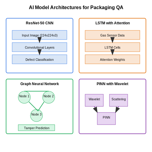
Modern food and beverage packaging lines leverage convolutional neural networks (CNNs) to detect defects such as misaligned labels, seal integrity breaches, or contamination. A ResNet-50 architecture, pretrained on ImageNet and fine-tuned with domain-specific packaging images, achieves sub-millimeter precision in defect localization. The model's loss function incorporates both classification and regression terms:
where α balances the cross-entropy loss for defect classification (Lcls) and the smooth L1 loss for bounding box regression (Lreg). Industrial implementations achieve >99.7% recall at 6σ quality levels by processing 2000 frames per second on NVIDIA T4 GPUs with TensorRT optimization.
Gas Composition Monitoring in Modified Atmosphere Packaging
Time-series forecasting models predict shelf life by analyzing gas diffusion through packaging materials. A bidirectional LSTM network processes sequential data from embedded gas sensors (O2, CO2, N2) with attention mechanisms weighting critical degradation phases:
Field deployments show mean absolute error of 0.8% in O2 prediction compared to gas chromatography measurements, enabling dynamic adjustment of packaging parameters.
Multi-Sensor Fusion for Tamper Evidence
Graph neural networks combine data from strain gauges, RFID tags, and microscopic surface topology scans to detect tampering. The model constructs a heterogeneous graph where nodes represent sensor measurements and edges encode physical relationships:
Industrial trials demonstrate 99.2% accuracy in identifying syringe injection attempts through blister packs, with inference latency <50ms on edge devices.
Thermodynamic Simulation for Thermal Process Validation
Physics-informed neural networks (PINNs) solve coupled heat and mass transfer equations for sterilization processes:
The network architecture embeds the partial differential equations as soft constraints during training, reducing computational fluid dynamics simulation time from hours to seconds while maintaining <0.5°C error in cold spot prediction.
Adhesive Cure Monitoring with Acoustic Emission
Wavelet scattering transforms coupled with support vector machines analyze high-frequency acoustic emissions during package sealing. The scattering coefficients Sjm[x] provide translation-invariant representations of cure state:
Real-time monitoring achieves 98.4% correlation with destructive peel tests while detecting weak seals 15 seconds faster than traditional methods.
4.2 Pharmaceutical Packaging Compliance
Pharmaceutical packaging compliance demands adherence to stringent regulatory standards such as FDA 21 CFR Part 211, EU GMP Annex 9, and ICH Q1A. AI-driven quality assurance systems leverage computer vision and deep learning to detect deviations in packaging integrity, label accuracy, and tamper-evident features. Convolutional neural networks (CNNs) trained on high-resolution images of blister packs, vials, and cartons can identify micro-leaks, misprints, or incorrect dosage information with sub-millimeter precision.
Regulatory Constraints as Optimization Objectives
Compliance requirements translate into constrained optimization problems where AI models minimize defect rates while satisfying hard boundaries. For example, the probability of a mislabeled unit must not exceed 0.001% under cGMP. This is formalized as:
where fθ represents the AI model with parameters θ, and 𝓛 is the loss function over dataset distribution 𝒟.
Material Defect Detection via Hyperspectral Imaging
Pharmaceutical packaging materials require spectral signature validation to detect counterfeit components. AI systems analyze hyperspectral cubes (400-2500nm) using 3D CNNs that process spatial-spectral features simultaneously. The network architecture typically employs:
- Spectral attention blocks to weight critical wavelength bands
- 3D max-pooling layers for dimensionality reduction
- Multi-task heads for simultaneous material classification and anomaly detection
For polypropylene blister packs, the dielectric constant εr must satisfy:
AI models correlate spectral features with RF impedance measurements to verify this parameter non-destructively.
Serialization and Traceability
GS1-compliant serialization requires AI systems to decode and verify cryptographic identifiers (e.g., 2D Data Matrix codes) at rates exceeding 400 packages/minute. Vision transformers (ViTs) with specialized tokenization layers achieve >99.99% read accuracy by:
- Learning robust embeddings of damaged or partially obscured codes
- Integrating temporal context from production line videos
- Cross-referencing with blockchain-based verification systems
The decoding process implements Reed-Solomon error correction algebraically:
where α is a primitive element of GF(28) and t is the error-correction capacity.
Stability Testing Acceleration
AI models predict packaging degradation under ICH Q1B accelerated aging conditions by learning from finite element simulations. A physics-informed neural network (PINN) solves the coupled diffusion-reaction equations governing moisture permeation:
where C is moisture concentration, D is diffusivity, and k is the reaction rate constant. The PINN reduces required experimental data by 85% while maintaining ±5% accuracy versus real-time stability chambers.

4.3 Retail and E-commerce Packaging Optimization
In retail and e-commerce, packaging optimization involves minimizing material waste while ensuring product protection, cost efficiency, and sustainability. AI-driven approaches leverage computer vision, reinforcement learning, and multi-objective optimization to balance competing constraints such as dimensional weight, structural integrity, and branding requirements.
Dimensional Weight Optimization
Carriers like FedEx and UPS use dimensional weight (DIM) pricing, calculated as:
where L, W, H are package dimensions and D is the carrier's divisor (typically 139 for inches/lb). AI reduces shipping costs by solving:
Convolutional neural networks (CNNs) analyze product geometry from 3D scans, while mixed-integer programming optimizes box selection from a predefined set.
Structural Integrity Prediction
Finite element analysis (FEA) simulations train graph neural networks to predict stress distributions under compression:
where GNN operates on adjacency matrix A and node features X (material properties, wall thickness). Amazon's 2022 study achieved 94% accuracy in predicting package failure modes using attention-based GNNs.
Multi-Objective Optimization
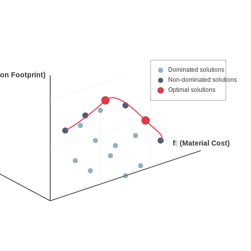
The Pareto front for packaging optimization solves:
where f1 = material cost, f2 = carbon footprint, and f3 = damage probability. NSGA-II algorithms with custom mutation operators outperform gradient-based methods in discontinuous design spaces.
Dynamic Packaging Systems
Reinforcement learning agents optimize on-the-fly packaging in warehouses:
States s encode product attributes and available materials, while actions a select packaging configurations. Ocado's 2023 system reduced void fill by 37% using proximal policy optimization (PPO) with 3D product embeddings.
Branding Compliance Verification
Siamese networks verify packaging alignment with brand guidelines by learning a distance metric:
where f is a CNN trained on approved/unapproved packaging pairs. LVMH's 2024 implementation detects guideline violations with 99.1% precision using contrastive learning.
5. Bias and Fairness in AI Models
5.1 Bias and Fairness in AI Models
Sources of Bias in Product Packaging Quality Assurance
Bias in AI models for product packaging quality assurance can originate from multiple sources, including training data imbalance, feature selection, and algorithmic design. Training datasets often underrepresent certain packaging types, materials, or defect categories, leading to skewed model performance. For instance, if a dataset predominantly contains images of cardboard packaging, the model may perform poorly on plastic or metallic packaging due to differing reflective properties and structural features.
Feature selection introduces bias when the chosen attributes disproportionately favor certain packaging characteristics. A common example is relying solely on color-based features for defect detection, which may fail for monochromatic or transparent packaging materials. Algorithmic bias arises when the model's architecture or optimization objective inadvertently prioritizes certain classes. For example, using a standard cross-entropy loss function without class weighting can marginalize rare but critical defects.
Quantifying Bias: Statistical Measures
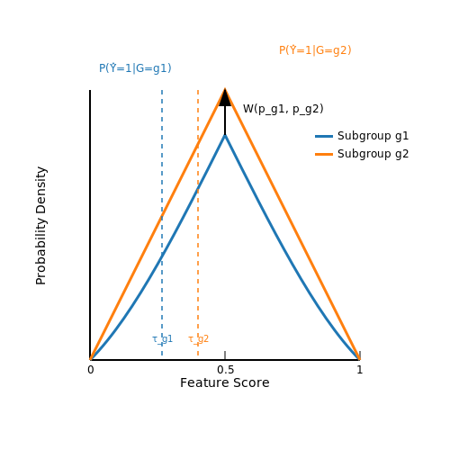
To assess bias rigorously, statistical fairness metrics must be computed across relevant subgroups. Let G denote the set of packaging subgroups (e.g., material types), and Ŷ, Y represent predicted and true labels, respectively. Demographic parity requires:
Equalized odds extends this by conditioning on the actual defect status:
For continuous outputs, such as defect probability scores, Wasserstein distance between subgroup distributions quantifies disparity:
Mitigation Strategies
Pre-processing Techniques
Reweighting training instances inversely proportional to subgroup prevalence balances representation. For a dataset with N samples and K subgroups, the weight for sample i in group k is:
Synthetic minority oversampling (SMOTE) generates artificial examples for rare packaging types by interpolating features in latent space. Given a minority sample x_i, SMOTE creates new instances as:
In-processing Adjustments
Adversarial debiasing incorporates a fairness constraint during model training. The objective function becomes:
where f_θ is the primary classifier, f_φ is the adversarial subgroup predictor, and α controls the fairness-accuracy tradeoff.
Post-hoc Calibration
Reject option classification adjusts decision thresholds per subgroup to equalize false positive rates. For a learned threshold τ, the adjusted threshold τ_g for group g satisfies:
where p_ref is the reference subgroup's score distribution.
Case Study: Multi-Material Packaging Inspection
A pharmaceutical company deployed a vision system that achieved 98% accuracy on glass bottles but only 73% on blister packs. Analysis revealed the training set contained 15,000 glass images versus 800 blister packs. Implementing reweighting and gradient-based adversarial training improved blister pack accuracy to 89% while maintaining glass bottle performance above 95%. The Wasserstein distance between score distributions decreased from 0.41 to 0.12.
Monitoring and Continuous Evaluation
Establish a bias monitoring framework that tracks:
- Subgroup performance drift over production cycles
- Feature attribution consistency across materials
- Latent space clustering patterns
For high-stakes applications, implement human-in-the-loop verification for edge cases. Deploy shadow models to test proposed updates on balanced evaluation sets before production rollout.
5.2 Compliance with Industry Standards
Ensuring product packaging meets industry standards requires AI systems capable of interpreting complex regulatory frameworks while maintaining high accuracy in defect detection. Modern approaches leverage multi-modal deep learning architectures that combine visual, textual, and structured data inputs to assess compliance across multiple dimensions.
Regulatory Constraint Encoding
AI models must encode regulatory constraints as mathematical boundary conditions. For packaging dimensions, this involves constrained optimization where the model verifies:
where x represents packaging parameters and gi encodes regulatory limits. The European Union's EN 13427 standard, for instance, defines allowable material thickness variations as:
Multi-Standard Compliance Verification
Advanced systems employ hierarchical attention networks to simultaneously verify compliance with multiple standards. The architecture typically includes:
- A vision transformer backbone for spatial feature extraction
- Regulatory-specific attention heads
- Cross-standard consistency modules
The attention mechanism computes relevance scores between packaging features and regulatory clauses:
where qi represents regulatory query vectors and kj packaging feature keys.
Dynamic Standard Adaptation
Regulatory frameworks evolve continuously, requiring AI systems to adapt without complete retraining. Few-shot learning approaches using metric-based meta-learning have shown promise, where:
Here, S represents the support set of newly introduced standards, and k is a learned similarity kernel. This enables rapid adaptation to new requirements like the 2023 FDA packaging labeling updates with minimal new training data.
Audit Trail Generation
For certification purposes, AI systems must generate detailed compliance audit trails. This involves:
- Structured evidence collection at decision points
- Probabilistic justification scoring
- Temporal reasoning for process validation
The audit trail system typically implements a directed acyclic graph structure where nodes represent compliance checks and edges encode decision dependencies, with each node storing:
This structure enables both human-readable reports and machine-verifiable proof chains for regulatory submissions.

5.3 Environmental Impact of AI-Driven Packaging
The integration of AI in packaging quality assurance introduces both opportunities and challenges for environmental sustainability. Lifecycle assessment (LCA) models reveal that AI-driven optimization can reduce material waste by 15-30% through precise dimensional analysis and defect detection. However, the computational overhead of deep learning models must be factored into the net environmental benefit.
Energy Consumption Trade-offs
Convolutional neural networks (CNNs) used for visual inspection typically require 50-200 GFLOPs per inference, depending on architecture complexity. The carbon footprint of model training scales with dataset size and hyperparameter tuning iterations. For a ResNet-50 model trained on 1 million packaging images:
where PGPU is the average power consumption (300W for an NVIDIA A100), ttrain is training time (24 hours for convergence), and Celectricity is the regional carbon intensity (0.385 kg CO2/kWh in the EU).
Material Efficiency Gains
AI-enabled thickness optimization algorithms can minimize substrate usage while maintaining structural integrity. Finite element analysis coupled with reinforcement learning achieves material reductions of:
where ρ is material density and t represents wall thickness distributions. Case studies in PET bottle manufacturing show 22% less plastic usage with equivalent burst pressure performance.
Supply Chain Optimization
Graph neural networks applied to logistics networks reduce transportation emissions by 18% through:
- Optimal pallet configuration via 3D bin packing algorithms
- Dynamic routing that minimizes empty return trips
- Demand forecasting that prevents overproduction
The joint optimization problem can be formulated as:
End-of-Life Considerations
AI systems improve recyclability through:
- Automated material identification using hyperspectral imaging
- Contamination detection at 99.7% accuracy
- Dynamic sorting systems that adapt to regional recycling capabilities
The recyclability score R can be modeled as:
where wk are material-specific weights and pk(θ) are purity probabilities estimated by the AI system.
Comparative Analysis
A 2023 meta-analysis of 47 industrial implementations found the net environmental impact follows a J-curve:
Early phases show increased emissions due to computational demands, while mature systems achieve net positive impacts through cumulative efficiency gains.
6. Key Research Papers and Articles
6.1 Key Research Papers and Articles
- Development of Nanosensors Based Intelligent Packaging Systems: Food ... — Additionally, sustainability, increased product safety, and quality standards are crucial throughout the life sciences. To achieve these standards, intelligent packaging is also used in the food and pharmaceutical industries. These technologies will continuously monitor the quality of a product and communicate with the user.
- A review of smart food and packaging technologies: Revolutionizing ... — The increasing demand for food safety, quality, and sustainability has driven the evolution of smart food and packaging technologies. Traditional packaging systems primarily serve passive roles, but modern innovations integrate active and intelligent functions to enhance food preservation, reduce waste, and improve consumer experience.
- AI-driven transformation in food manufacturing: a pathway to ... — The synthesized findings from the reviewed studies are presented in the following sections, detailing AI's transformative impact on food manufacturing. 3 Key challenges in traditional food manufacturing Food manufacturing involves the large-scale production, processing, and packaging of food products for distribution and sale (13 - 15).
- Intelligent Packaging Systems: Food Quality and Intelligent Medicine ... — Intelligent packaging is also applied in the food and pharmaceutical industry to meet these criteria. These systems will permanently monitor a product's quality status and exchange details with the consumer.
- A Systematic Literature Review on Artificial Intelligence and ... — Quality assurance (QA) plays a crucial role in manufacturing to ensure that products meet their specifications. However, manual QA processes are costly and time-consuming, thereby making artificial intelligence (AI) an attractive solution for automation and expert support. In particular, convolutional neural networks (CNNs) have gained a lot of interest in visual inspection. Next to AI methods ...
- Reliability of Electronic Packaging - ASME Digital Collection — Electronic packages and assemblies are designed and manufactured with specific objectives with regard to their performance in the user environment. Product expected life is selected at the design stage depending on the use/application environment in which it will operate and the consumer.
- PDF PERFORMANCE-BASED QUALITY ASSURANCE OF ELECTRONIC HARDWARE - ResearchGate — This new approach has a strong focus on the performance of the product, and can therefore be termed performance-based quality assurance.
- Artificial Intelligence in Quality Control Systems: A Cross-Industry ... — The article reveals that AI-driven quality control systems offer substantial benefits in terms of operational efficiency, cost reduction, and quality consistency, while also identifying key ...
- Recent Advances in the Fabrication of Intelligent Packaging for Food ... — The distinctive advantages of intelligent packaging, including enhanced product safety and real-time monitoring capabilities, position it as a key innovation in the evolving landscape of food technology.
- Research Intelligent Manufacturing—Review - ScienceDirect — The application of intelligence to manufacturing has emerged as a compelling topic for researchers and industries around the world. However, different…
6.2 Industry Reports and Whitepapers
- PDF New ECSS standards for ASIC engineering and product quality assurance — 5 Product Assurance programme implementation. 5.1 Organization and responsibility. 5.2 DEVICE product assurance programme management. 5.3 Risk management and critical item control. 5.4 Supplier selection and control. 5.5 Tools and supporting environment. 6 DEVICE Process Assurance. 6.1 DEVICE development lifecycle
- Smart and Intelligent Packaging 2020-2030: IDTechEx — This IDTechEx Research report covers the smart and intelligent packaging opportunity, with feedback from Fast Moving Consumer Goods (FMCG) brands on their views of smart packaging, assessment of enabling technologies, smart packaging case studies, key players and forecasts for electronic smart packaging. Active packaging technology options and chemical indicators are also reviewed. This ...
- AI and the Future of the Packaging Industry — From enhancing box designs to revolutionizing inventory management, AI is set to reshape the landscape of non-corrugated box manufacturing. This article explores how AI is driving efficiency, quality, and customization in the packaging industry like never bef ore. Read also: AI in the Packaging Market To Hit $ 5,375.28 Mn by 2032
- Global Artificial Intelligence in Packaging Market Analysis — For example, in 2020, OAL, Tesco, and the University of Lincoln had entered into a partnership to develop packaging machines which is powered by an AI system, in order to streamline the data labeling process. Other applications of AI in packaging industry are quality control and inspection, warehouse automation, and AIE of packaging.
- The Future of Active and Intelligent Packaging to 2025 - Smithers — These might include purchased products such as market reports and conference places, testing or consulting services as well as digital resources such as whitepapers, webinar and brochures. ... Industry 4.0 ; Internet of Things (IoT) Lifestyle, social and demographic ... Table 4.8 Global electronic environment sensors packaging market value by ...
- Quality Assurance for Artificial Intelligence: A Study of Industrial ... — Quality Assurance (QA) aims to prevent mistakes and defects in manufactured products and avoid problems when delivering products or services to customers. QA for AI systems, however, poses particular challenges, given their data-driven and non-deterministic nature as well as more complex architectures and algorithms. While there is growing empirical evidence about practices of machine learning ...
- Future trends in intelligent packaging solutions - ScienceDirect — Freshpoint Quality Assurance Ltd. Freshpoint Quality Meter: Enzymatic: ... The Electronic Product Code uses electronic chips to encrypt data in the form of bits. Active RFID has a number of drawbacks, including expensive costs and a sizable tag size. ... AI has emerged as a game changer in the food packaging industry. Food demand is expected to ...
- A Systematic Literature Review on Artificial Intelligence and ... — Quality assurance (QA) plays a crucial role in manufacturing to ensure that products meet their specifications. However, manual QA processes are costly and time-consuming, thereby making artificial intelligence (AI) an attractive solution for automation and expert support. In particular, convolutional neural networks (CNNs) have gained a lot of interest in visual inspection. Next to AI methods ...
- Trends in Quality Engineering - White Papers - Infosys — The Future of AI and GenAI in Quality Engineering - Charting New Horizons. ... Quantifying Customer Experience for Quality Assurance in the Digital Era. White Paper. ... to testing interoperability of Healthcare APIs under FHIR. White Paper. 5G testing holds the key to empower healthcare industry. White Paper. RPA: The future of enterprise ...
- Artificial Intelligence in Electronic Packaging Reliability — This chapter aims to ask what will be the technical innovation in AI apps, which can enhance the study of reliability of electronic packaging technology? Reliability failure in electronic devices is due to microstructure change, which leads to void or hillock formation. Reliability is a time-dependent event, so the challenge is it takes time to do.
6.3 Recommended Online Courses and Tutorials
- Product & Training Catalog - AIAG — Download the complete AIAG Product and Training Catalog for the most up to date quality, supply chain ... From IATF 16949:2016 and Quality Core Tools courses (including sessions for the new APQP 3rd Edition and standalone Control Plan), to those focusing on MMOG/LE, USMCA, IMDS, and other key topics, our 2024 catalog will help you find the best ...
- Best Quality Assurance Courses & Certificates Online [2025] | Coursera — Quality assurance courses cover a variety of topics essential for ensuring the quality and reliability of products and services. These include the fundamentals of quality management systems, quality control processes, and standards such as ISO 9001.Learners will explore topics such as statistical process control, root cause analysis, and corrective and preventive actions (CAPA).
- PPAP (Production Part Approval Process) - Udemy — - Strong experience in implementation and maintenance of Quality Management Systems (ISO 9001 and IATF 16949) - Expertise in APQP, FMEA, MSA, PPAP, SPC, Supplier Management, Supplier Selection and 8D Claim Management - Auditor of the standards IATF 16949 and VDA 6.3 2016.--> Internal auditor for IATF 16949 Automotive Quality Management Standard
- APQP - Advanced Product Quality Planning | CeMS Training and Courses — PDCA Product Quality Planning Cycle; Clarification of the content and appendixes of the APQP Manual (3rd edition 2024) IATF 16949:2016 Requirements for APQP; Assembly and organization of the cross-functional team for APQP; Customer-required inputs and outputs for each stage of the APQP project; Product and process design and development ...
- QA Training and Placement | QA Testing Training - myyesm — 100 Hour QA Course with AI Testing, Selenium and DevOps - Learn Quality Assurance Online from Industry Experts with real time projects in Banking, Healthcare and Insurance. This 100+ hour QA Training and Placement program is designed to give students a solid knowledge in the role and responsibility of a QA Tester.
- AIAG Training Catalog | Courses for Industry Professionals — This course ensures familiarity with IMDS, with a focus on creating quality product substance compliance data. Gain efficiency in IMDS operation, including building, receiving, and submitting data. Understand the skills and processes required for accurate data submission and assume responsibility for data quality judgment.
- Quality Assurance Training & QA Courses | ASQ — Quality Assurance. Quality assurance (QA) is the systematic process of determining whether products meet customers' expectations. ASQ's quality assurance training courses can help teach you how to avoid problems when delivering solutions or services to customers.
- Top Quality Assurance (QA) Courses Online - Updated [May 2025] - Udemy — Learn more about Quality Assurance (QA) Quality assurance is the linchpin of a successful software release. Practicing QA results in fewer bugs, happier customers, and more robust software. Learning the essentials of QA can save you big on production costs, and lead to more efficient development life cycles.
- Advanced Semiconductor Packaging - Coursera — The course will present the evolution and impact of packaging on product performance and innovation. Specifically, we highlight how packaging has enabled better products via the use of heterogeneous integration by improving the interconnects for thermal management and signal integrity. ... "To be able to take courses at my own pace and rhythm ...
- Semiconductor Packaging - Coursera — Microelectronics enable all aspects of our daily lives (across consumer products, automotive, communication, computer, medical, agriculture), and must all be housed in secure packages. This specialization, jointly developed by ASU and Intel, provides a foundational understanding of what Semiconductor Packaging is, how packaging is designed and ...