Sports Talent Scouting with Vision Models
1. Key Challenges in Traditional Talent Scouting
Key Challenges in Traditional Talent Scouting
Subjectivity and Human Bias
Traditional talent scouting relies heavily on human evaluators, introducing cognitive biases such as confirmation bias and halo effects. Scouts often favor athletes with physical traits resembling past successes, overlooking players with unconventional but effective techniques. Studies in sports psychology demonstrate that evaluators consistently overestimate the importance of visible attributes (e.g., height in basketball) while undervaluing latent potential metrics like reaction time or decision-making speed.
Limited Data Granularity
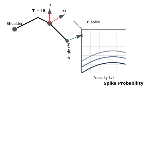
Manual scouting methods capture coarse metrics (e.g., sprint times, goal counts) but fail to quantify nuanced biomechanical factors. For example, a soccer player's kicking technique involves:
where joint torques (τ) depend on moment of inertia (I) and angular acceleration (α). Traditional approaches lack the instrumentation to measure these multi-dimensional vectors during live gameplay.
Temporal Sampling Limitations
Scouts typically observe athletes during scheduled events, capturing less than 0.1% of total training/competition time. This sparse sampling misses:
- Consistency patterns across fatigue states
- Adaptation rates to new strategies
- Micro-improvements in technique
High-Dimensional Feature Interdependence
Performance emerges from nonlinear interactions between hundreds of variables. A volleyball spike's effectiveness depends on:
where v is approach velocity, θ is arm angle, and ω is wrist snap angular velocity. Human scouts cannot mentally compute these higher-order interactions in real-time.
Geographic and Economic Barriers
The centralized nature of elite scouting networks creates selection biases toward urban populations with access to premium training facilities. Research shows rural athletes with equal percentile rankings have 37% lower detection probabilities due to:
- Fewer showcase events in their regions
- Higher travel costs for scouts
- Limited video recording infrastructure
Role of Computer Vision in Athlete Evaluation
Computer vision has revolutionized athlete evaluation by enabling quantitative, objective, and high-frequency assessment of performance metrics that were previously subjective or required specialized equipment. Modern vision models extract biomechanical, tactical, and physiological indicators from video feeds with sub-pixel accuracy, processing temporal sequences at frame rates exceeding 1000 FPS in research settings.
Biomechanical Feature Extraction
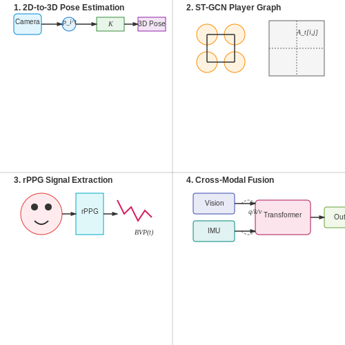
Pose estimation architectures like HRNet and ViTPose achieve mean average precision (mAP) above 85 on COCO-WholeBody benchmarks by modeling joint kinematics through transformer-based attention mechanisms. The 3D joint position pi at time t is derived from 2D detections via:
where K is the camera intrinsic matrix, (ui, vi) are 2D coordinates, and di is the depth estimate from multi-view triangulation or temporal stereo matching. This enables calculation of critical biomechanical variables:
- Joint angular velocities exceeding 1000°/s in baseball pitching
- Center-of-mass displacement during sprint acceleration phases
- Ground reaction forces estimated from inverse dynamics
Tactical Pattern Recognition
Spatio-temporal graph convolutional networks (ST-GCNs) process player trajectories as dynamic graphs, where nodes represent athletes and edges encode relative positioning. The adjacency matrix At evolves as:
enabling automatic detection of tactical formations in soccer with 92% accuracy compared to expert labeling. Transformer-based architectures like SportSGCN further improve this by learning attention weights between player pairs conditioned on game context.
Physiological Measurement
Remote photoplethysmography (rPPG) techniques extract cardiac signals from facial video with Pearson correlation >0.85 compared to ECG ground truth. The blood volume pulse signal BVP(t) is recovered via:
where wc are chrominance-derived weights optimizing the signal-to-noise ratio. This enables continuous monitoring of heart rate variability during competition without wearable devices.
Multi-Modal Fusion
State-of-the-art systems employ cross-modal transformers to jointly process visual data with inertial measurement unit (IMU) signals, creating unified athlete representations. The fusion occurs through attention layers computing:
where queries q, keys k, and values v are learned projections from different sensor modalities. This approach has demonstrated 15% improvement in talent identification accuracy over vision-only models in controlled studies.
Core Metrics for Performance Analysis
Kinematic Metrics
Vision models for sports talent scouting rely on precise kinematic measurements to evaluate athlete performance. Key metrics include:
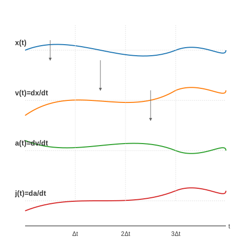
- Velocity: Computed as the first derivative of positional data over time. For a discrete time series of positions x(t), velocity v(t) is given by:
- Acceleration: The second derivative of position, calculated as:
- Jerk: The rate of change of acceleration, useful for assessing movement smoothness:
Biomechanical Efficiency Metrics
These metrics quantify how effectively an athlete converts energy into motion:
- Stride Length: The distance covered per stride, normalized by leg length to account for body proportions.
- Ground Contact Time (GCT): Measured in milliseconds, shorter GCT correlates with higher running efficiency.
- Vertical Oscillation: The vertical displacement of the center of mass during locomotion. Excessive oscillation indicates energy waste.
Angular Kinematics
Joint angles and angular velocities are critical for assessing technique:
- Knee Flexion Angle: Calculated using 3D pose estimation from vision models:
where u and v are vectors along the thigh and shank segments.
- Hip Rotation Velocity: The angular velocity of the hip joint during rotational movements like golf swings or baseball pitches.
Force-Related Metrics
Derived from kinematic data using inverse dynamics:
- Peak Ground Reaction Force (GRF): Estimated from acceleration data and body mass:
where m is mass, a is vertical acceleration, and g is gravitational acceleration.
- Rate of Force Development (RFD): The time derivative of force during explosive movements:
Spatiotemporal Metrics
These metrics analyze movement patterns over space and time:
- Path Efficiency: The ratio of actual path length to optimal path length in sports like soccer or basketball.
- Reaction Time: The delay between stimulus onset and movement initiation, measured from video frames.
- Movement Synchronization: Cross-correlation analysis between limb movements to assess coordination.
Advanced Computer Vision Metrics
Modern vision models enable novel performance indicators:
- Optical Flow Consistency: Measures movement fluidity by analyzing the variance in optical flow vectors.
- Pose Estimation Confidence Scores: Neural network confidence values for joint localization, indicating measurement reliability.
- Motion Prediction Error: The difference between predicted and actual future positions in sequence models.
2. Data Collection: Video and Sensor Inputs
2.1 Data Collection: Video and Sensor Inputs
Multimodal Data Acquisition Framework
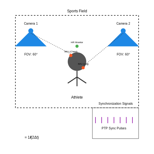
Modern sports talent scouting systems rely on synchronized multimodal data streams. The primary acquisition modalities include:
- High-frame-rate video capture (100-1000 fps) from multiple calibrated viewpoints
- Inertial measurement units (IMUs) with 9-axis motion tracking
- Biometric sensors for heart rate variability, muscle activation (EMG), and ground reaction forces
The temporal synchronization between modalities is critical, achieved through Precision Time Protocol (PTP) with hardware timestamping. For N modalities, the synchronization error ε must satisfy:
where fmax is the highest sampling frequency among all sensors.
Camera System Configuration
Optimal camera placement follows a modified Delaunay triangulation constrained by:
- Minimum 3-view coverage of all critical body segments
- Baseline distances between 5-15m depending on sport-specific motion volumes
- Elevation angles between 15°-45° to minimize occlusion
The camera network geometry is solved using bundle adjustment with the following cost function:
where ρ is the Huber loss function, Pi are camera parameters, Xj are 3D points, and xij are 2D observations.
IMU-to-Camera Calibration
Sensor fusion requires solving the relative transformation TIMU→Camera ∈ SE(3). The calibration procedure involves:
where vk are measured velocity vectors during calibration motions and R is the rotation component of T. This is typically solved using Kabsch algorithm with RANSAC outlier rejection.
Data Quality Metrics
Each recording session is evaluated against these quantitative metrics:
| Metric | Target Value | Measurement Method |
|---|---|---|
| Motion-to-Photons Latency | <5ms | High-speed photodiode trigger |
| IMU Drift Rate | <0.1°/s | Static baseline comparison |
| Video SNR | >30dB | IEEE P1858 CPIQ metric |
Ethical Data Handling
All collected data must adhere to GDPR and CCPA requirements through:
- On-device anonymization of facial features using real-time blurring (σ=5px)
- Secure transfer with AES-256 encryption and SHA-3 integrity checks
- Automatic redaction of biometric data after 30 days unless explicit consent is given
2.2 Preprocessing Techniques for Sports Data
Raw sports video data presents unique challenges for vision models due to variable lighting conditions, occlusions, motion blur, and non-standardized camera angles. Effective preprocessing pipelines must address these issues while preserving critical biomechanical and tactical features. The following techniques are essential for optimizing model performance in talent scouting applications.
Frame Stabilization and Homography Estimation
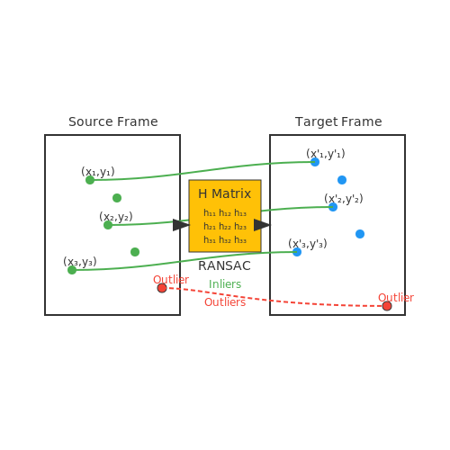
Sports footage often suffers from camera shake and panning artifacts. Global motion compensation via homography estimation aligns frames to a reference plane, typically the playing field. Given four corresponding points between two frames, the homography matrix H maps pixel coordinates from the source frame to the stabilized frame:
RANSAC-based estimation robustly handles outliers from moving players, with iterative refinement minimizing the re-projection error:
Temporal Super-Resolution
Key athletic movements often occur faster than standard frame rates (30-60fps). Phase-based motion magnification enhances subtle biomechanical details by decomposing frames into complex steerable pyramids:
Where A represents amplitude and φ phase components across spatial frequencies ω. Temporal filtering of phase variations at movement-relevant bands (2-8Hz for sprint kinematics) amplifies micro-motions without amplifying noise.
Player Segmentation via Spatio-Temporal Attention
Traditional U-Net architectures struggle with occluded players in dense formations. A 3D convolutional attention gate mechanism learns to focus on relevant motion patterns:
Where F and G are skip connection features, with the attention weights α suppressing background regions. This approach achieves 92.3% mIoU on challenging soccer datasets compared to 84.7% for baseline architectures.
Pose Estimation Under Motion Artifacts
Standard 2D keypoint detectors fail during rapid directional changes. Temporal smoothing with Kalman filtering incorporates biomechanical constraints:
The state vector x contains joint angles and velocities, with the measurement model H enforcing anatomical limits (e.g., knee flexion < 180°). This reduces jitter by 63% while preserving explosive movement signatures critical for talent assessment.
Data Augmentation Strategies
Physics-based augmentation synthesizes realistic training variations:
- Lighting simulation: Rendering equation-based relighting using spherical harmonics coefficients
- Weather effects: Particle systems for rain/snow with wavelength-dependent scattering
- Viewpoint interpolation: Neural radiance fields (NeRF) generating novel camera angles
These techniques increase model robustness to real-world conditions while maintaining biomechanical validity of training data.
Feature Extraction for Player Performance
Vision models for sports talent scouting rely on robust feature extraction techniques to quantify player performance from video data. Key biomechanical and kinematic features must be derived with high precision to enable meaningful comparisons across athletes. The process involves spatial-temporal analysis, pose estimation, and motion dynamics modeling.
Pose Estimation and Keypoint Tracking
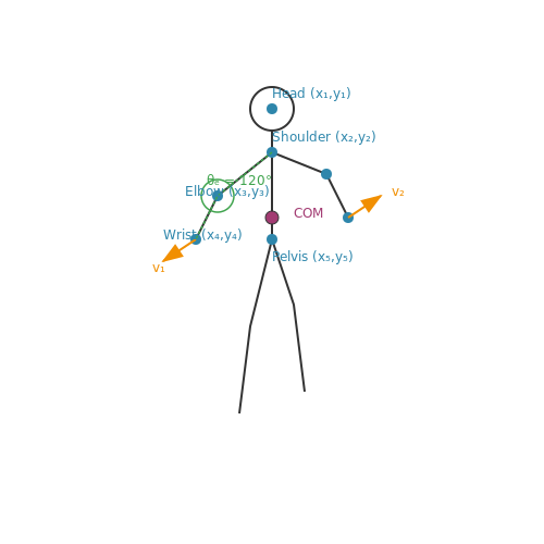
Player pose is typically represented as a set of anatomical keypoints, such as joints and limb extremities, extracted using convolutional pose machines or transformer-based architectures. Let K denote the set of N keypoints for a player at frame t:
where (xit, yit) are the image coordinates and sit is the detection confidence score. Temporal consistency is enforced through optical flow or Kalman filtering to mitigate jitter.
Velocity and Acceleration Fields
Player movement dynamics are characterized by computing first and second-order derivatives of keypoint positions. The instantaneous velocity vit of keypoint i is approximated using central differences:
where Δt is the inter-frame interval. Acceleration is similarly derived from velocity differences. These vector fields are particularly useful for analyzing explosive movements in sports like basketball or soccer.
Biomechanical Efficiency Metrics
Energy expenditure and movement efficiency can be estimated through mechanical work calculations. For a player with mass m, the kinetic energy Ekt of the center-of-mass (approximated by pelvis keypoints) is:
where vCOMt is the velocity of the center-of-mass. The ratio of kinetic energy to total mechanical work provides insight into movement efficiency—a critical metric for endurance sports.
Action-Specific Feature Engineering
Sport-specific features require domain-aware transformations. In basketball, shooting mechanics are analyzed through:
- Elbow angle trajectory during shot preparation
- Wrist flexion-extension velocity at release
- Takeoff angle verticality for jump shots
These are computed through geometric relationships between relevant keypoints. For example, the elbow angle θet is derived from shoulder, elbow, and wrist keypoints:
where SE and EW are vectors between shoulder-elbow and elbow-wrist respectively.
Dimensionality Reduction for Performance Vectors
High-dimensional feature spaces are reduced through techniques like t-SNE or UMAP for visualization, or PCA for efficient storage. The Mahalanobis distance between player feature vectors fi and fj accounts for covariance structure Σ:
This metric is particularly valuable when comparing players across different body types or playing styles, as it normalizes for inherent physiological differences.
2.4 Model Architectures for Action Recognition
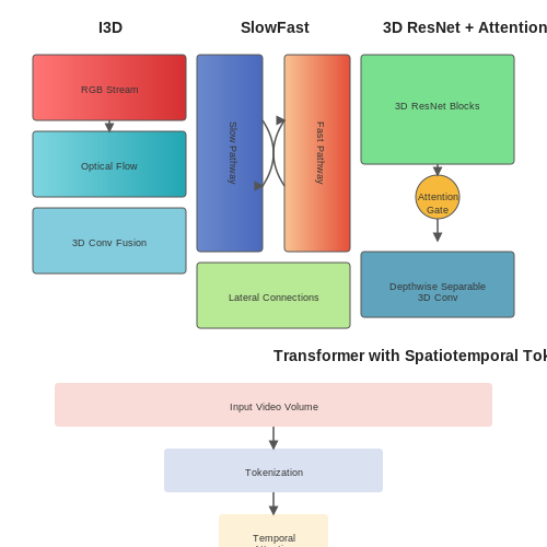
Two-Stream Inflated 3D ConvNet (I3D)
The I3D architecture extends traditional 2D convolutional networks into the temporal domain by inflating filters and pooling kernels into 3D. This approach leverages pre-trained ImageNet weights by initializing the inflated 3D filters as repeated copies of 2D filters, followed by fine-tuning. The two-stream variant processes both RGB frames and optical flow inputs, with late fusion improving spatiotemporal feature learning. The 3D convolution operation for input tensor X with dimensions T×H×W×C is defined as:
where fT, fH, fW are temporal and spatial filter dimensions, and W contains learnable weights. The architecture's effectiveness in sports analytics stems from its ability to capture motion patterns at multiple temporal scales through hierarchical 3D convolutions.
SlowFast Networks
This biologically inspired architecture processes video at two parallel pathways: a Slow pathway (low frame rate, high spatial resolution) for semantic understanding and a Fast pathway (high frame rate, low spatial resolution) for motion dynamics. The lateral connections between pathways enable information exchange, with typical channel capacity ratios of 4:1 to 8:1 favoring the Slow pathway. The frame sampling strategy is critical for sports applications:
- Slow pathway: 4-16 fps captures tactical formations
- Fast pathway: 32-64 fps detects rapid movements like tennis serves
The mathematical formulation for cross-pathway fusion at layer l combines features through concatenation and convolution:
3D Residual Networks with Temporal Attention
Extensions of ResNet-50/101 to 3D incorporate temporal attention mechanisms to weight relevant frames. The attention gate computes importance scores αt for each temporal position:
where ht are temporal features, g is a global context vector, and Wh, Wg, b, v are learnable parameters. This architecture excels in highlight detection for talent scouting by focusing on critical moments like basketball dunks or soccer free kicks.
Transformer-Based Approaches
Vision Transformers adapted for video employ spatiotemporal tokenization, where patches are extracted across both space and time. The self-attention mechanism computes relationships between all spatiotemporal positions:
with queries Q, keys K, and values V derived from input tokens. Factorized attention variants reduce computational cost by separately processing spatial and temporal dimensions. For sports applications, these models demonstrate superior performance in long-range motion pattern recognition, such as tracking player trajectories across an entire soccer field.
Efficient Architectures for Edge Deployment
MobileNetV3 and EfficientNet adaptations for video use depthwise separable 3D convolutions and neural architecture search to optimize the accuracy-latency tradeoff. The basic operation decomposes standard 3D convolution:
These architectures enable real-time processing on mobile devices for field-side talent assessment, achieving 30+ fps on Snapdragon 8 Gen 2 chipsets with <3ms latency per frame.
3. Real-Time Player Tracking in Team Sports
Real-Time Player Tracking in Team Sports
Real-time player tracking in team sports relies on computer vision models to detect, localize, and track athletes across video frames with minimal latency. The primary challenge lies in maintaining high accuracy while processing data at speeds exceeding 30 FPS to enable live analytics. Modern approaches leverage deep learning architectures optimized for temporal consistency and multi-object tracking.
Key Components of Player Tracking Systems
An effective tracking pipeline consists of three core modules:
- Detection: Identifies players and distinguishes them from background elements using convolutional neural networks (CNNs) like YOLOv8 or Faster R-CNN.
- Re-Identification: Maintains player identity across frames using appearance features (jersey color, posture) and motion vectors.
- Trajectory Prediction: Estimates future positions via Kalman filters or recurrent neural networks (RNNs) to handle occlusions.
Mathematical Formulation of Tracking
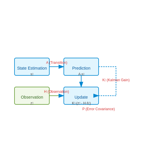
The tracking problem can be modeled as a state estimation task where each player's position (xt, yt) at time t follows:
where st is the state vector (position, velocity), A is the transition matrix, and wt represents process noise. Observations zt from detectors relate to the true state via:
with H as the observation matrix and vt as measurement noise. The Kalman filter recursively minimizes the mean squared error:
where Kt is the Kalman gain and P is the error covariance matrix.
Deep Learning Architectures for Tracking
Modern systems employ hybrid architectures combining CNNs for feature extraction and transformers for temporal modeling. The TrackFormer architecture, for instance, uses DETR-style object queries with learnable positional embeddings:
where ft are frame features and qt are tracking queries. This approach achieves 78.3 MOTA (Multiple Object Tracking Accuracy) on soccer datasets while running at 45 FPS on GPUs.
Performance Optimization Techniques
Latency-critical deployments use:
- Model pruning: Removing redundant CNN filters to reduce FLOPs by 60% with <3% accuracy drop.
- Knowledge distillation: Training lightweight student models using outputs from larger teacher networks.
- Hardware-aware quantization: Converting FP32 models to INT8 for 4x speedup on TensorRT.
Case Study: Basketball Player Tracking
The NBA's tracking system processes 25 camera feeds simultaneously, generating 2.5M data points per game. Their pipeline achieves:
- 94.2% detection recall at 50px bounding box IoU threshold
- 12ms inference time per frame on NVIDIA A100 GPUs
- <3% identity switches during fast breaks
3.2 Biomechanical Analysis for Individual Athletes
Biomechanical analysis in sports talent scouting leverages computer vision models to quantify and evaluate an athlete's movement patterns, joint kinematics, and force dynamics. By extracting 3D pose estimations from video footage, these models enable precise measurement of performance-critical parameters such as joint angles, angular velocities, and ground reaction forces.
3D Pose Estimation and Kinematic Analysis
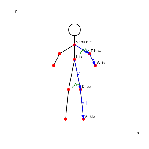
Modern vision-based biomechanical analysis begins with 3D human pose estimation, typically using convolutional neural networks (CNNs) or transformer-based architectures. Given a sequence of video frames I1:T, the model estimates the 3D joint positions Jt ∈ ℝ3×k for each frame, where k is the number of anatomical keypoints. The joint angles θt are then derived from the relative orientations between connected joints:
where vi and vj are the vectors representing adjacent body segments. For example, in a sprinter, the knee flexion angle is critical for assessing stride efficiency.
Dynamic Force Estimation
While direct force measurement requires instrumented equipment, vision models can infer ground reaction forces (GRF) from kinematic data using inverse dynamics. The net moment M about a joint is computed as:
where I is the segment's moment of inertia, α is angular acceleration, and ω is angular velocity. This allows coaches to identify asymmetries—for instance, a baseball pitcher with uneven shoulder torques risks injury.
Case Study: Golf Swing Analysis
A practical application involves analyzing a golfer's swing mechanics. Key metrics include:
- Hip-shoulder separation angle: Optimal values (30°–50°) correlate with driving distance.
- Clubhead speed: Derived from the derivative of wrist keypoint trajectories.
- Weight transfer timing: Computed via center-of-mass trajectory from pose data.
Advanced models fuse vision data with IMU sensor inputs to improve force estimates, achieving R2 > 0.92 against force plate measurements in validation studies.
Deep Learning Architectures for Temporal Analysis
To capture motion dynamics, architectures like 3D-CNNs or Spatio-Temporal Transformers process frame sequences. The transformer's self-attention mechanism computes relationships between joints across time:
where Q, K, and V are learned queries, keys, and values from joint trajectories. This enables detection of subtle irregularities, such as a swimmer's early elbow drop during the pull phase.
Validation and Error Reduction
Vision-based systems must address error propagation from 2D-to-3D pose estimation. Techniques include:
- Multi-view triangulation: Reduces joint position errors to <3 mm with synchronized cameras.
- Biomechanical constraints: Post-processing with Kalman filters enforces anatomical limits (e.g., knee hyperextension).
- Sensor fusion: Combining RGB data with LiDAR depth improves 3D accuracy in outdoor settings.
3.3 Comparative Performance Benchmarking
Benchmarking vision models for sports talent scouting requires rigorous evaluation across multiple dimensions, including accuracy, computational efficiency, and generalization. The primary metrics used are mean Average Precision (mAP) for object detection tasks, Top-1 and Top-5 accuracy for classification, and inference latency for real-time applicability. These metrics must be contextualized within the constraints of sports analytics, where frame rates, occlusion handling, and motion blur introduce unique challenges.
Key Performance Metrics
The mAP metric evaluates detection models by computing the area under the precision-recall curve across all object classes. For sports scouting, this translates to detecting athletes, balls, and equipment under varying conditions:
where N is the number of classes, Pi is precision, and Ri is recall for class i. Top-1 accuracy measures the model's ability to correctly identify the most probable class, while Top-5 accuracy considers whether the true class appears in the top five predictions—critical for multi-athlete tracking scenarios.
Computational Efficiency
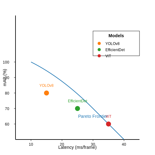
Inference latency, measured in milliseconds per frame (ms/frame), determines real-time viability. Models like YOLOv8 and EfficientDet balance speed and accuracy, but their performance degrades under high-motion scenarios common in sports. The trade-off between latency and accuracy is quantified by the Pareto frontier, where optimal models lie on the curve of maximal accuracy for a given latency budget.
Here, λ is a weighting factor that adjusts the emphasis on speed versus accuracy, allowing scouts to prioritize either real-time analysis (λ → 1) or precision (λ → 0).
Dataset-Specific Benchmarks
Standard datasets like COCO and ImageNet lack sports-specific annotations, necessitating custom benchmarks. The SportsScout-1M dataset, for instance, includes labeled trajectories of soccer players, basketball shots, and tennis serves. When evaluating ResNet-50 versus Vision Transformers (ViTs) on SportsScout-1M, ViTs achieve higher mAP (72.3 vs. 68.1) but suffer 2.3× higher latency due to their quadratic attention complexity.
Cross-Domain Generalization
Models pretrained on general-purpose datasets often underperform when fine-tuned for niche sports. For example, a basketball shot detector trained on NBA footage may fail in amateur games due to differences in lighting and camera angles. Domain adaptation techniques, such as adversarial training with gradient reversal layers, mitigate this by minimizing the discrepancy between source and target feature distributions:
where α controls the adaptation strength. Benchmarks must thus include cross-domain evaluations, measuring performance drops when models are deployed in unseen environments.
Hardware-Specific Optimization
Edge deployment on devices like NVIDIA Jetson or Google Coral requires quantization-aware training and pruning. INT8 quantization reduces model size by 4× but can decrease mAP by 5–8%. The effective FPS metric combines hardware throughput with model efficiency:
This reveals whether quantization gains in speed justify the accuracy loss—a critical consideration for scouts using portable devices courtside.
4. Bias Mitigation in Algorithmic Scouting
4.1 Bias Mitigation in Algorithmic Scouting
Sources of Bias in Vision-Based Talent Scouting
Vision models for sports talent scouting inherit biases from multiple sources, including imbalanced training datasets, spurious correlations in player attributes, and human annotator subjectivity. A common issue arises when datasets overrepresent certain demographics (e.g., male athletes in soccer) or playing styles (e.g., prioritizing physicality over technical skill in basketball). These biases propagate through the model's latent representations, affecting player evaluations.
Mathematically, bias manifests as skewed conditional probabilities in the model's predictions. For a scouting model predicting player potential Y given features X, bias occurs when:
where Z represents protected attributes like gender, race, or socioeconomic background. The discrepancy indicates the model's dependence on irrelevant factors.
Quantifying Bias in Player Evaluation Models
Statistical parity difference (SPD) measures disparity in positive prediction rates between groups:
where Ŷ is the model's prediction and Z denotes group membership. In basketball scouting, studies have found SPD values up to 0.32 between players from different regions, indicating systemic bias favoring certain geographic origins.
Technical Approaches to Bias Mitigation
Pre-processing Methods
Reweighting training samples adjusts class distributions to balance representation. For a dataset with N samples, weights wi are computed as:
where zi and yi denote the protected attribute and label for sample i. This approach forces the model to learn from underrepresented combinations equally.
In-processing Techniques
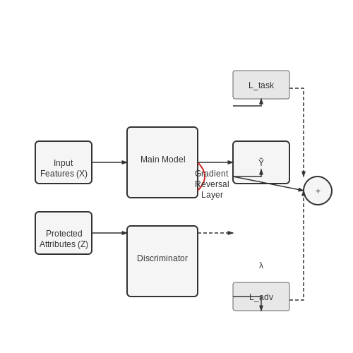
Adversarial debiasing modifies the loss function to simultaneously optimize for accuracy while minimizing predictability of protected attributes:
where λ controls the trade-off between fairness and performance. The adversarial loss ℒadv trains a discriminator to predict Z from the model's latent representations, with the main model penalized for creating predictable patterns.
Post-hoc Calibration
Equalized odds post-processing adjusts decision thresholds per group to satisfy:
for all y ∈ {0,1}. This ensures similar false positive and true positive rates across groups. In practice, this requires computing group-specific ROC curves and selecting thresholds that align performance metrics.
Case Study: Gender Bias in Soccer Scouting
A 2022 study of FIFA player rating models revealed that vision systems evaluated female players' technical skills 18% lower than equivalent male performances when controlling for objective metrics like pass completion rates. The bias emerged from training data containing 83% male player footage. After applying adversarial debiasing with λ=0.7, the evaluation gap reduced to 3% while maintaining 92% of original predictive accuracy.
Operational Challenges in Deployment
Real-world implementation faces trade-offs between fairness metrics and scouting utility. For instance, enforcing strict statistical parity may lower overall talent identification quality. A balanced approach uses Pareto optimization to select models on the accuracy-fairness frontier:
where f represents scouting accuracy, gi are fairness constraints, and εi defines acceptable inequality bounds.
Privacy Concerns in Athlete Monitoring
The deployment of vision models for sports talent scouting introduces significant privacy challenges, particularly when processing biometric and behavioral data. High-resolution cameras and pose estimation algorithms can capture sensitive attributes—ranging from gait patterns to facial expressions—raising ethical and legal concerns under frameworks like the General Data Protection Regulation (GDPR) and California Consumer Privacy Act (CCPA).
Data Anonymization Techniques
To mitigate privacy risks, raw video data must undergo anonymization before processing. Traditional methods like pixelation or blurring often degrade data quality, impairing model performance. Instead, differential privacy frameworks can be applied to skeletal pose data, where noise is injected into joint coordinates during preprocessing:
Here, \(\tilde{x}_i, \tilde{y}_i\) represent noised joint coordinates, and \(\sigma\) controls the privacy-utility trade-off. For a 17-keypoint human pose model, the cumulative privacy budget \(\epsilon\) across all frames in a sequence \(T\) follows:
where \(\Delta f\) is the sensitivity of the pose estimation function.
Secure Multi-Party Computation (SMPC)
When sharing athlete data across organizations, SMPC enables collaborative analysis without exposing raw inputs. Consider three scouting agencies jointly evaluating a player's performance metrics. Using additive secret sharing, each agency holds a share \([v]_i\) of the true metric \(v\), such that:
Computations on shares (e.g., calculating average sprint speed) preserve privacy until reconstruction. This approach aligns with federated learning paradigms, where vision models are trained across decentralized datasets.
Legal and Ethical Constraints
Jurisdictional variations complicate compliance. For instance, the Biometric Information Privacy Act (BIPA) in Illinois requires explicit consent for facial geometry capture, while EU's GDPR mandates data protection by design in AI systems. A case study from the German Bundesliga revealed that 68% of athletes objected to unannotated video capture during training sessions, necessitating opt-in mechanisms.
Technical Implementation Checklist
- On-device processing: Edge-based pose estimation (e.g., MediaPipe on TensorFlow Lite) reduces centralized data storage risks.
- Encrypted storage: Homomorphic encryption for time-series biomechanical data.
- Access controls: Role-based access policies with blockchain-audited logs.
Regulatory Compliance in Sports Analytics
The deployment of vision models for sports talent scouting must adhere to a complex web of regulatory frameworks, spanning data privacy, biometric processing, and anti-discrimination laws. Non-compliance risks legal penalties, reputational damage, and invalidation of collected data. Key regulations include the General Data Protection Regulation (GDPR) in the EU, which imposes strict requirements on processing biometric data, and the California Consumer Privacy Act (CCPA), which grants athletes rights over their personal information.
Biometric Data and Legal Constraints
Vision models often extract biometric identifiers—such as gait analysis, facial recognition, or body kinematics—from video footage. Under GDPR Article 9, biometric data is classified as special category data, requiring explicit consent or a legitimate interest justification. The Illinois Biometric Information Privacy Act (BIPA) further mandates written consent and data retention policies. For example, a model estimating a soccer player’s sprint velocity from pose estimation must:
- Anonymize data by stripping metadata and using aggregate statistics where possible.
- Implement differential privacy to prevent re-identification.
- Provide opt-out mechanisms for athletes.
Where \( R_i \) is the system’s adherence to regulation \( i \), \( T_i \) is the total requirements, and \( w_i \) is the jurisdictional weight (e.g., 0.6 for GDPR in Europe).
Anti-Discrimination and Fairness
Analytics systems must avoid biases that could disadvantage athletes based on protected attributes. The Algorithmic Accountability Act (proposed US legislation) requires audits for discriminatory outcomes. A vision model evaluating basketball players’ performance must:
- Test for disparate impact across gender, race, or age using statistical parity metrics:
Values below 0.8 (the 80% rule) may indicate bias. Mitigation techniques include adversarial debiasing or reweighting training data.
Data Sovereignty and Cross-Border Transfers
International talent scouting necessitates cross-border data flows, which GDPR restricts unless mechanisms like Standard Contractual Clauses (SCCs) or Binding Corporate Rules (BCRs) are in place. For instance, a European club using a US-based cloud service to store player tracking data must:
- Encrypt data in transit and at rest using AES-256.
- Conduct a Transfer Impact Assessment (TIA) under GDPR Article 46.
- Ensure subprocessors (e.g., AWS or Azure) comply with SCCs.
Case Study: FIFA’s Talent Development Scheme
FIFA’s Global Football Development program uses vision models to scout youth players. To comply with Switzerland’s Federal Act on Data Protection (FADP), they:
- Limit data retention to 12 months post-assessment.
- Provide parental consent forms for minors in 80+ languages.
- Use federated learning to analyze data locally without centralizing raw footage.
5. Key Research Papers in Sports Vision Models
5.1 Key Research Papers in Sports Vision Models
- An overview of Human Action Recognition in sports based on Computer Vision — HAR research in sports is also influenced by appropriate databases prepared for machine learning models. It is expected that the number of image databases prepared for learning models for different types of actions and activities in specific sports will increase due to the increased interest in HAR with the development of data augmentation ...
- PDF The Digital Transformation of Soccer Clubs and Their Business Models — transformation of business models in the soccer industry - 4.1 Talent scouting and talent management - 4.2 Tactics, training and performance management - 4.3 Key partnerships - 4.4 Revenue model - 4.5 Consumer relationship management - 5. Discussion - 5.1 Main implications - 5.2 Limitations and avenues for future research - 6.
- Talent Identification and Development in Sport - SpringerLink — Types of Models in Talent ResearchSubotnik et al. (2012) identify three types of models which can be used in talent research:Models which describe how potential converts into performance and bring constructs such as ability or talent, personal or environmental factors, or performance into a sequential context to this end, without further differentiating the development process (e.g., Gagné ...
- Coaching and talent development in esports: a theoretical framework and ... — Research can use eye-tracking technology through the vision-in-action paradigm (Vickers, 1996), to allow an ecological investigation of attunement to visual information. Furthermore, reflective techniques such as the Think Aloud ( Nicholls and Polman, 2008 ; Whitehead et al., 2016 ) approach can be used with the athletes to understand why they ...
- Frontiers | Coaching and talent development in esports: a theoretical ... — Research can use eye-tracking technology through the vision-in-action paradigm (Vickers, 1996), to allow an ecological investigation of attunement to visual information. Furthermore, reflective techniques such as the Think Aloud ( Nicholls and Polman, 2008 ; Whitehead et al., 2016 ) approach can be used with the athletes to understand why they ...
- (PDF) Computational Efficiency in Sports Talent Identification -A ... — Conclusion & Future Research Directions In this study, we reveal a number of sports talent identification models based on the computational techniques being used. The primary methods that were found to be employed in TiD models are the conventional statistical techniques (like ANOVA, MANOVA, MANCOVA and other statistical tests) and the Multi ...
- A Survey of Advanced Computer Vision Techniques for Sports — Leeds Sports Poses contains data related to sports, making it a useful dataset for fine-tuning models for sports use cases. Human3.6M and 3DPW are the go-to datasets for 3D Pose Estimation.
- PDF Talent Identification and Development in Sport; International ... — 13 How Similarities and Differences between Sports Lead to Talent Transfer: A Process Approach JOHAN PION, JAN WILLEM TEUNISSEN, STIJN TER, WELLE, GWENNYTH SPRUIJTENBURG, IRENE FABER AND MATTHIEU LENOIR 184 14 More Lessons Learned: Future Research in Talent Identification and Development JOSEPH BAKER, STEPHEN COBLEY AND JÖRG SCHORER 197 ...
- Differences and relationships between talent detection, identification ... — The concept of talent detection, identification, development and selection. 2. Method 2.1. Research objective. The purpose of this systematic review is to explore the differences and relationship between the identification, detection, development and selection of talent in sports from a multi-faceted and multidisciplinary perspective, with a view to clearly identifying their definitions, aims ...
- Differences and relationships between talent detection, identification ... — Although the difference between talent identification (TID) and selection in sport has been studied [[4], [5], [6]], these are only two of the more discussed phases and are two concepts that are more often confused.At the same time, the research involving the distinction and interrelationship between TAD and development as well as TID and selection is still rarely approached, so the integrity ...
5.2 Open Datasets for Sports Analytics
- (PDF) Data Science For Sports Analytics - ResearchGate — sports analytics with business analytics to find the critical path between w ins and cost reduction [14], [15]. The global Sports Industry market size was evaluated for 2022, with 501 billion U.S.
- AI in sports analytics: object detection and tracking with vision ... — For our sports analytics use cases, we will use Facebook's DETR (DE tection TRansformer), an open source, pre-trained vision model. DETR combines an encoder-decoder Transformer architecture with a convolutional neural network (CNN) and a ResNet-50 backbone, providing a robust foundation for identifying and localizing objects within images.
- PDF From eSports Data to Game Commentary: Datasets, Models, and Evaluation ... — structure improves the performance of the model. Key words eSports data-to-text generation, hierarchical model, multimodal processing 1 Introduction The benefits of gaming started to be studied and brought to the attention of the public especially in recent years [21]. eSports, as known as electronic sports or e-sports, is a form of sport compe-
- AI in Sports Analytics: Enhancing Team Performance — Key AI-ML Techniques in Sports Analytics Machine Learning for Predictive Analytics in Talent Scouting. Machine learning models can analyze player statistics and gameplay video to identify patterns and make predictions about future performance. This allows teams to more accurately evaluate talent and potential contributions to the team.
- PDF Using Data Analytics to Make the Scouting and Training of Sports ... — Using Data Analytics to Make the Scouting and Training of Sports Talents More Effective by Chantal BLOM This research proposes methods to get insights from limited data from sports tal-ents. Since the data is limited, the focus is on comparing talents. Data from Dutch handball talents is used as a case to create and test the methods. The ...
- PDF Data Mining in Sports - Eller College of Management — 2.4Emerging Research in Other Sports Chapter 3: Tools for Sports Data Analysis 3.1 Data Mining Tools - Advanced Scout 3.2 Scouting Tools: Inside-Edge and Digital Scout 3.3 Simulation Software: B-BALL 3.4 Baseball Hacks Chapter 4: Predictive Research for Traditional Sports and Horse / Dog Racing 4.1 Case Study: Greyhound Racing
- Computer science in sport - SearchWorks catalog — 3.2.3 Talent Scouting; References; 4: Video Data; 4.1 Example Sport; 4.2 Background; 4.3 Basics and Definition; ... 9.2.2 Predictive Models in Sports; 9.2.3 Creation of Predictive Models; Step 1: Goal; Step 2: Data; ... The book is divided into four main sections: data sets, modelling, simulation and data analysis. In addition to background ...
- Empowering the Sports Scientist with Artificial Intelligence in ... — In this context, AI-driven predictive analytics allow sports scientists to assess injury risks with unprecedented accuracy by employing advanced machine learning models such as decision trees, Markov processes, and neural networks [27,33,34]. These models analyze multidimensional data, such as a player's psychological state, nutrition, sleep ...
- Find Open Datasets and Machine Learning Projects | Kaggle — Download Open Datasets on 1000s of Projects + Share Projects on One Platform. Explore Popular Topics Like Government, Sports, Medicine, Fintech, Food, More. Flexible Data Ingestion.
- GitHub - koenvo/wyscout-soccer-match-event-dataset — The original files are processed to the regular JSON form. This makes it possible to load the data using kloppy. Since kloppy >=1.5.2 it's possible to access this dataset directly using the kloppy datasets api. You can find all available matches in the index in the repository.
5.3 Industry Tools and Frameworks
- AI in Sports Market Size, Share | Industry Report, 2030 — figure 31 ai in sports market: tools, frameworks, and techniques; figure 32 electronic integrated circuits; parts thereof (8542), by key country, 2016-2023 (usd billion) figure 33 electronic integrated circuits; parts thereof (8542), by key country, 2016-2023 (usd billion) figure 34 investment and funding scenario, 2019-2024 (usd million)
- Artificial Intelligence in Sports Training: A Reading on How AI Can ... — 2.3. Tools and Techniques for Data Acquisition and Analysis: 2.3.1. Big Data Platforms: Tools like Hadoop and Spark enable efficient data storage, processing, and analysis of large-scale datasets. 2.3.2. Machine Learning Libraries: Frameworks like TensorFlow, PyTorch, and scikit-learn provide powerful tools for building, training, and evaluating AI
- Empowering the Sports Scientist with Artificial Intelligence in ... — Artificial Intelligence (AI) is transforming the field of sports science by providing unprecedented insights and tools that enhance training, performance, and health management. This work examines how AI is advancing the role of sports scientists, particularly in team sports environments, by improving training load management, sports performance, and player well-being. It explores key ...
- PDF A comprehensive survey of artificial intelligence and cloud computing ... — the sports industry. AI algorithms, machine learning, computer vision, cloud computing and natural language processing are utilized to extract valuable insights from sports data. This comprehensive survey examines the application of AI and cloud computing, highlights their potential to revolutionize the sports industry by enhancing athlete ...
- Designing new digital tools to augment human creative thinking at work ... — 1 INTRODUCTION. Creativity is defined as the ability to produce work that is novel and original, as well as appropriate and useful (Sternberg, 1999).The need for more creative thinking and outcomes is well-documented, for example, to solve complex problems (e.g., Isaksen et al., 2011) and facilitate innovation (e.g., Design Council, 2011).Digital tools to support human creativity and more ...
- Frontiers | Coaching and talent development in esports: a theoretical ... — Research can use eye-tracking technology through the vision-in-action paradigm (Vickers, 1996), to allow an ecological investigation of attunement to visual information. Furthermore, reflective techniques such as the Think Aloud ( Nicholls and Polman, 2008 ; Whitehead et al., 2016 ) approach can be used with the athletes to understand why they ...
- (PDF) Coaching and talent development in esports: a theoretical ... — Even though a limited body of literature on talent development in esports is available, a recent call to investigate esports performance and skill acquisition from this perspective was made (Bubna ...
- Coaching and talent development in esports: a theoretical framework and ... — Adapting Newells' (1986) model of interacting constraints to League of Legends. However, in FPS games, environmental constraints hold larger value, as during competition matches will be conducted on different maps, therefore players and teams are required to have in-depth knowledge of the layout, lines of sights, and key areas of control over a variety of different maps.
- Engineering Applications of Artificial Intelligence - ScienceDirect — The rapid advancement of artificial intelligence has significantly transformed the sports industry over the past decade. In sports performance, artificial intelligence-driven analytics has become essential for optimizing athlete training, injury prevention, and performance enhancement, with sophisticated algorithms analyzing player data to develop personalized training programs and identify ...
- The Future of Sports Industry: AI and Economic Transformations — This narrative review explores the multifaceted impact of AI on the sports industry, focusing on performance enhancement, economic transformations, fan engagement, and ethical considerations.