Transformer Block Dissected Layer-by-Layer
1. Core Components of a Transformer
Core Components of a Transformer
Multi-Head Attention Mechanism
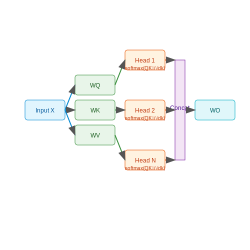
The multi-head attention mechanism is the cornerstone of the transformer architecture, enabling the model to process input sequences in parallel while capturing diverse relationships between tokens. Given an input sequence X of dimension n × dmodel, the mechanism projects X into queries (Q), keys (K), and values (V) using learned weight matrices:
where WQ, WK, WV ∈ ℝdmodel × dk. The scaled dot-product attention computes compatibility scores between queries and keys, scaled by √dk to prevent gradient vanishing:
Multi-head attention concatenates h parallel attention heads, each with unique projection matrices, allowing the model to attend to different positional and contextual features simultaneously. The output is linearly transformed:
Position-Wise Feed-Forward Networks
Each transformer block contains a feed-forward network (FFN) applied independently to every token position. The FFN consists of two linear transformations with a ReLU activation in between, expanding the inner dimension to dff = 4dmodel before projecting back:
This architecture enables the model to learn complex non-linear transformations while maintaining positional invariance, as the same parameters are shared across all positions.
Layer Normalization and Residual Connections
Transformers employ residual connections followed by layer normalization (LN) around both the attention and FFN sub-layers. For a sub-layer S with input x, the output is computed as:
Layer normalization stabilizes training by normalizing activations across the feature dimension (dmodel), unlike batch normalization which operates across the batch dimension. The residual pathways mitigate vanishing gradients in deep networks.
Positional Encoding
Since transformers lack recurrent or convolutional operations, positional encodings inject information about token order. The original paper uses sinusoidal functions of varying frequencies:
where pos is the position and i is the dimension. These encodings allow the model to attend by relative positions and generalize to sequences longer than those seen during training.
Masking in Decoder Layers
Decoder blocks utilize masked self-attention to prevent positions from attending to subsequent tokens during autoregressive generation. This is implemented by adding a mask M to the attention scores before softmax, where Mij = -∞ if i < j and 0 otherwise:
1.2 Self-Attention Mechanism Overview
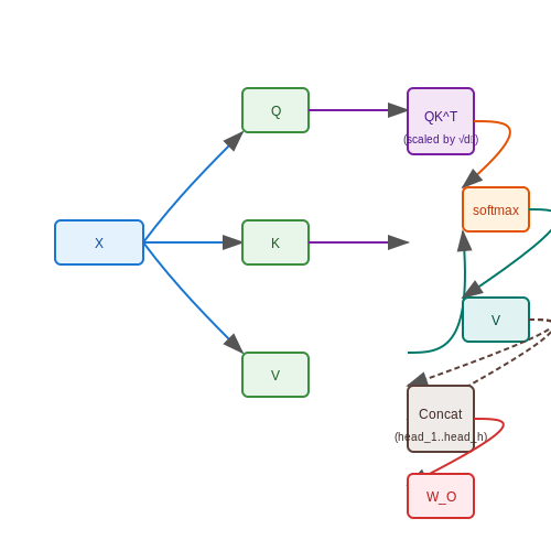
The self-attention mechanism computes a weighted sum of input representations, where the weights are dynamically derived based on pairwise interactions between all elements in the sequence. Given an input sequence X ∈ ℝn×d with n tokens and d-dimensional embeddings, self-attention first projects X into three matrices:
where WQ, WK, WV ∈ ℝd×dk are learnable projection matrices. The query (Q), key (K), and value (V) matrices enable the model to compute attention weights by measuring compatibility between each query and all keys.
Scaled Dot-Product Attention
The core operation computes attention scores as scaled dot products between queries and keys, followed by softmax normalization:
The scaling factor √dk prevents gradient vanishing issues when dk is large, as the dot products grow in magnitude. The softmax ensures the attention weights sum to 1 along each row, creating a convex combination of values.
Multi-Head Attention
Multi-head attention extends this process by applying h independent attention heads in parallel. Each head learns distinct projections, enabling the model to jointly attend to information from different representation subspaces:
where headi = Attention(QWQi, KWKi, VWVi), and WO ∈ ℝhdv×d is the output projection matrix. Typical implementations use h = 8 heads with dk = dv = d/h.
Computational Complexity
Self-attention exhibits O(n2d) time and space complexity due to the QKT matrix multiplication. While this allows direct modeling of long-range dependencies, it becomes computationally prohibitive for very long sequences, motivating sparse or linear attention variants in recent research.
Positional Encoding
Since self-attention is permutation-invariant, sinusoidal positional encodings are added to input embeddings to inject sequential order information:
where pos is the position and i is the dimension. These encodings enable the model to attend by relative or absolute positions while maintaining translation equivariance.
1.3 Positional Encoding and Embeddings
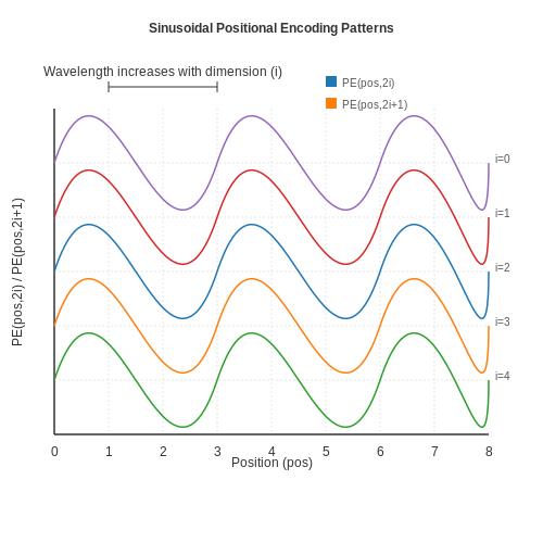
Transformers process input tokens in parallel, unlike recurrent architectures that inherently capture sequential order through recurrence. To inject positional information into the model, Vaswani et al. introduced sinusoidal positional encodings, which are added to token embeddings before being fed into the transformer layers. The encoding for position pos and dimension i is defined as:
where dmodel is the embedding dimension. The wavelengths form a geometric progression from 2π to 20000π, allowing the model to learn both fine-grained and coarse positional relationships. The sinusoidal nature ensures that relative positions can be represented via linear transformations, enabling the model to generalize to sequence lengths longer than those seen during training.
Properties of Positional Encodings
The sinusoidal encoding has several key advantages:
- Boundedness: The values are constrained between [-1, 1], preventing numerical instability.
- Uniqueness: Each position has a unique encoding due to the sinusoidal functions' orthogonality.
- Relative Position Awareness: The dot product between two positional encodings depends only on their relative distance, not absolute positions.
Learned Positional Embeddings
An alternative approach is to use learned positional embeddings, where each position is assigned a trainable vector. While simpler, these embeddings:
- Lack theoretical guarantees for extrapolation to longer sequences.
- Require sufficient training data to learn meaningful positional relationships.
In practice, sinusoidal encodings are preferred for tasks requiring strong generalization to varying sequence lengths, while learned embeddings may perform better when training data is abundant and sequence lengths are consistent.
Embedding Layer
The token embeddings project discrete input tokens into a continuous dmodel-dimensional space. For a vocabulary of size V, the embedding matrix We ∈ ℝV × dmodel is learned during training. The combined input representation is:
where PE is the positional encoding matrix. This sum allows the model to jointly leverage semantic and positional information throughout the transformer layers.
Practical Considerations
Modern implementations often include:
- Layer normalization applied after the embedding sum to stabilize training.
- Dropout on the embeddings to prevent overfitting.
- Scale factors to control the relative contribution of embeddings and positional encodings.
For multilingual models, language-specific embedding layers may be used, with shared positional encodings across languages to enable cross-lingual transfer learning.
2. Multi-Head Self-Attention Layer
Multi-Head Self-Attention Layer
The multi-head self-attention (MHSA) mechanism is the cornerstone of the transformer architecture, enabling the model to jointly attend to information from different representation subspaces at different positions. Unlike single-head attention, MHSA projects the input into multiple subspaces, computes attention in parallel, and concatenates the results.
Mathematical Formulation
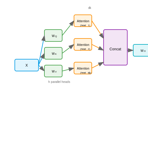
Given an input sequence X ∈ ℝn×d where n is the sequence length and d is the embedding dimension, MHSA first projects X into h sets of queries, keys, and values using learned linear transformations:
where WiQ, WiK, WiV ∈ ℝd×dk are learnable weight matrices for head i, and typically dk = d/h.
Scaled Dot-Product Attention
Each head computes scaled dot-product attention independently:
The scaling factor 1/√dk prevents the dot products from growing too large in magnitude, which would push the softmax into regions with extremely small gradients.
Concatenation and Projection
The outputs of all h attention heads are concatenated and projected back to the original dimension:
where WO ∈ ℝhdv×d is the output projection matrix and typically dv = dk = d/h.
Parallel Computation Efficiency
In practice, all heads are computed in parallel by batching the matrix multiplications. The entire MHSA operation can be implemented as:
where WQ, WK, WV are stacked versions of the individual head projections.
Interpretability Benefits
Different attention heads often learn to focus on different linguistic or structural patterns. Some heads may attend to local syntactic relationships while others capture long-range dependencies or specific positional patterns. This diversity contributes to the model's ability to process complex hierarchical structures in the input.
Computational Complexity
The time and space complexity of MHSA is O(n2d) due to the attention matrix computation. For long sequences, this quadratic complexity becomes prohibitive, motivating research into sparse attention variants and other optimizations.
2.2 Layer Normalization and Residual Connections
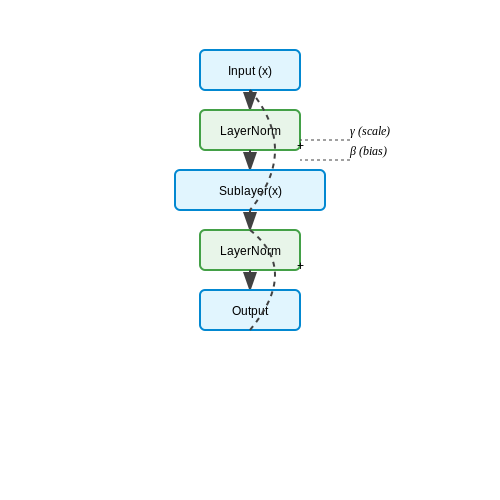
Layer normalization (LayerNorm) and residual connections are critical components in transformer architectures, enabling stable training of deep networks. Unlike batch normalization, which normalizes across the batch dimension, LayerNorm operates on individual samples, making it suitable for variable-length sequences common in natural language processing.
Layer Normalization Formulation
Given an input vector x ∈ ℝd, LayerNorm computes:
where γ and β are learnable affine parameters, and ε is a small constant for numerical stability (typically 10-5). The normalization is applied independently to each position in the sequence.
Residual Connections
Residual connections address the vanishing gradient problem in deep networks by creating shortcut paths for gradient flow. In transformers, each sub-layer (attention or feed-forward) employs:
This differs from the original ResNet formulation where normalization follows the residual path. The transformer variant, called post-normalization, places LayerNorm after the residual addition.
Gradient Flow Analysis
Consider the gradient through a residual block with input x and function F:
The term (1 + ∂F(x)/∂x) ensures gradients can propagate directly when ∂F(x)/∂x ≈ 0, preventing exponential decay through multiple layers.
Practical Implementation Considerations
- Initialization: Affine parameters γ are typically initialized to 1 and β to 0
- Precision: LayerNorm requires float32 precision to avoid instability in variance calculation
- Sequence Length Variance: Unlike batch normalization, LayerNorm produces consistent outputs regardless of batch composition
Comparative Analysis with Other Normalization Schemes
| Method | Normalization Axis | Batch Size Sensitivity | Sequence Length Sensitivity |
|---|---|---|---|
| BatchNorm | Batch × Features | High | None |
| LayerNorm | Features | None | None |
| InstanceNorm | Features | None | High |
Recent variants like RMSNorm eliminate the mean-centering operation, showing comparable performance with reduced computation:
In transformer architectures, the combination of LayerNorm and residual connections typically allows stable training of networks with hundreds of layers, whereas networks without these components often fail to converge beyond 10-20 layers.
2.3 Feed-Forward Neural Network Layer
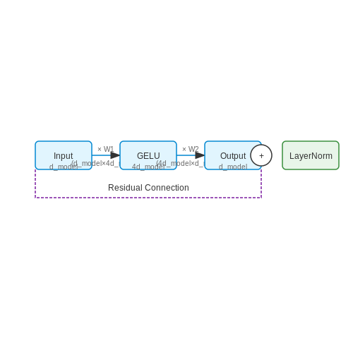
The Feed-Forward Neural Network (FFNN) layer in a Transformer block operates independently on each position from the multi-head attention output, applying the same transformation across all positions. This layer consists of two linear transformations with a Gaussian Error Linear Unit (GELU) activation in between, formulated as:
Where W1 ∈ ℝdmodel×dff and W2 ∈ ℝdff×dmodel are learnable weight matrices, with dff typically being 4×dmodel. The GELU activation function provides smooth nonlinearity and is defined as:
where Φ(x) is the standard Gaussian cumulative distribution function. This activation has shown superior performance in Transformer architectures compared to ReLU, particularly in language modeling tasks.
Dimensionality Considerations
The FFNN layer serves two primary purposes: first, it introduces additional capacity beyond the attention mechanism; second, it provides a channel for position-wise information processing. The expansion to dff = 4×dmodel creates a bottleneck architecture that:
- Enables richer representations in the hidden space
- Maintains computational efficiency through matrix multiplication optimizations
- Allows for better gradient flow during backpropagation
Practical Implementation Details
Modern implementations often employ fused operations for efficiency. The complete FFNN computation can be optimized as:
where both linear transformations include bias terms. In practice, the first linear layer expands the dimension from dmodel to dff, while the second contracts back to dmodel, maintaining dimensional consistency with the residual connection.
Initialization and Normalization
Weight matrices are typically initialized using Xavier/Glorot initialization with gain adjusted for the GELU activation. Layer normalization is applied before the FFNN in the original Transformer architecture (Pre-LN), though some variants use Post-LN:
The choice affects training dynamics, with Pre-LN generally providing more stable gradients in deep networks.
Computational Complexity
The FFNN layer contributes significantly to the overall compute requirements. For a sequence of length n and model dimension d, the complexity is:
This becomes the dominant term in longer sequences where n > d, motivating research into more efficient alternatives like grouped linear transformations or sparse expert networks.
Combining Components: The Full Transformer Block
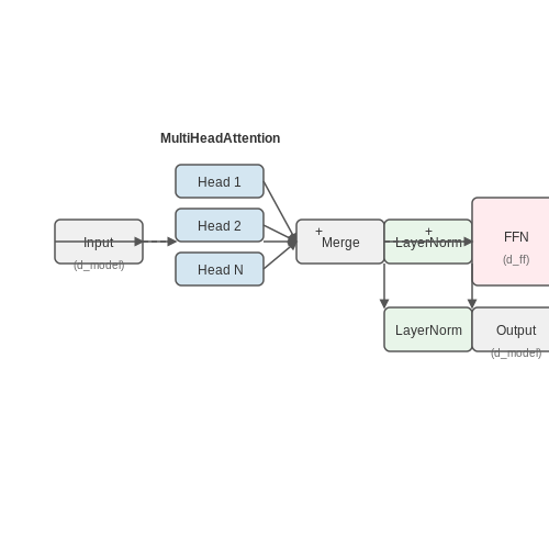
The transformer block integrates multiple sub-layers into a cohesive computational unit, enabling the model to process sequential data with self-attention and feed-forward transformations. Each component operates in sequence, with residual connections and layer normalization ensuring stable gradient flow during training.
Architecture Overview
A single transformer block consists of the following components in order:
- Multi-head self-attention mechanism
- Residual connection followed by layer normalization
- Position-wise feed-forward network
- Second residual connection followed by layer normalization
The complete forward pass through a transformer block can be expressed mathematically as:
Residual Connections and Layer Normalization
Each sub-layer employs residual connections that add the input directly to the output of the sub-layer before normalization. This architecture choice:
- Mitigates vanishing gradients in deep networks
- Preserves original signal information through the network
- Enables training of very deep transformer stacks
Layer normalization is applied to the sum of the residual connection and sub-layer output:
where the normalization operation standardizes activations across the feature dimension:
with learnable parameters γ and β, and statistics computed per sample across features.
Feed-Forward Network Details
The position-wise feed-forward network consists of two linear transformations with a ReLU activation in between:
where W₁ ∈ ℝ^{d_model × d_ff}, W₂ ∈ ℝ^{d_ff × d_model}, and typically d_ff = 4 × d_model. This expansion-reduction pattern allows for richer intermediate representations while maintaining input/output dimensionality.
Practical Implementation Considerations
When implementing transformer blocks in deep learning frameworks, several optimizations are commonly employed:
- Pre-LayerNorm: Some variants apply layer normalization before rather than after residual connections for improved training stability
- Dropout: Applied to attention weights and feed-forward activations for regularization
- Mixed Precision Training: Using FP16/FP32 hybrid precision to reduce memory usage
- Memory-Efficient Attention: FlashAttention or memory-efficient kernels for long sequences
The computational complexity of a single transformer block is dominated by the self-attention mechanism:
for sequence length n and model dimension d, making optimizations critical for long-sequence processing.
3. Hyperparameter Tuning for Transformer Blocks
3.1 Hyperparameter Tuning for Transformer Blocks
Key Hyperparameters in Transformer Blocks
The performance of transformer models is highly sensitive to their hyperparameters. The most critical ones include:
- Number of layers (depth): Determines the model's capacity to learn hierarchical representations. Deeper models can capture more complex patterns but risk overfitting and vanishing gradients.
- Hidden dimension size: Controls the width of feed-forward layers and embedding spaces. Larger dimensions increase model expressivity but also computational cost.
- Number of attention heads: Affects the model's ability to focus on different aspects of the input simultaneously. More heads allow for richer attention patterns but require more memory.
- Dropout rate: Regularization parameter that prevents overfitting by randomly deactivating neurons during training.
- Learning rate: Governs the step size during gradient descent optimization.
Mathematical Foundations of Hyperparameter Effects
The relationship between hyperparameters and model performance can be formalized through the transformer's computational complexity. The total number of parameters in a transformer block is given by:
where \( d_{model} \) is the hidden dimension, \( d_{ff} \) is the feed-forward layer dimension, and \( H \) is the number of attention heads. The computational complexity scales as:
for sequence length \( n \), hidden dimension \( d \), and \( L \) layers. This quadratic dependence on sequence length explains why longer contexts require careful hyperparameter selection.
Empirical Tuning Strategies
Effective hyperparameter tuning combines theoretical understanding with empirical validation:
- Learning rate warmup: Gradually increase the learning rate over the first \( k \) steps to stabilize early training. The optimal warmup period \( k \) typically scales with model size.
- Attention head allocation: For models with \( d_{model} = 768 \), empirical studies show optimal performance with 12 heads, maintaining \( d_k = d_v = 64 \) per head.
- Layer normalization placement: Pre-layer normalization generally outperforms post-layer normalization for deep transformers.
Automated Hyperparameter Optimization
Modern approaches leverage Bayesian optimization and evolutionary algorithms:
where \( \theta \) represents the hyperparameters and \( \mathcal{L} \) is the validation loss. Population-based training maintains multiple configurations simultaneously, exploiting cross-configuration information.
Case Study: BERT-Style Models
The original BERT architecture established several hyperparameter conventions:
- Base model: \( L = 12 \), \( d_{model} = 768 \), \( H = 12 \), \( d_{ff} = 3072 \)
- Large model: \( L = 24 \), \( d_{model} = 1024 \), \( H = 16 \), \( d_{ff} = 4096 \)
These configurations maintain an approximate 4:1 ratio between \( d_{ff} \) and \( d_{model} \), a pattern observed across many successful transformer variants.
Memory-Efficient Configurations
For resource-constrained applications, key tradeoffs include:
- Reducing \( d_{ff} \) while increasing \( d_{model} \) preserves total parameters but changes the model's inductive bias
- Using grouped query attention reduces memory usage from \( O(Hd^2) \) to \( O(Gd^2) \) where \( G \) is the number of query groups
- Gradient checkpointing enables training deeper models by trading compute for memory
Temperature Scaling in Attention
The attention softmax temperature \( \tau \) affects the sharpness of attention distributions:
Lower \( \tau \) values produce sharper distributions, while higher values yield more uniform attention. Optimal \( \tau \) typically falls between 0.1 and 1.0, depending on the task.
3.2 Common Pitfalls and Debugging Tips
Vanishing Gradients in Deep Transformer Stacks
Despite residual connections, deep Transformer models (e.g., >24 layers) can suffer from gradient attenuation during backpropagation. The issue stems from the multiplicative nature of gradient flow through multiple attention and feed-forward layers. For a model with L layers, the gradient norm scales as:
where λl represents the residual connection strength and σW the weight initialization variance. When λl approaches 1 (strong residuals), gradients stabilize, but improper initialization can still cause decay. Debugging steps:
- Monitor gradient norms per layer using hooks
- Verify residual scaling factors (typically 1/√L)
- Switch to Xavier/Glorot initialization if using vanilla linear layers
Attention Head Collapse
Multi-head attention sometimes exhibits "head collapse," where certain attention heads learn identical or near-identical patterns. This reduces model capacity and is detectable via:
- Cosine similarity >0.9 between query/key matrices across heads
- KL divergence <0.1 between attention distributions
Countermeasures include:
- Orthogonal initialization of projection matrices
- Adding a diversity loss term:
$$ \mathcal{L}_{div} = \sum_{i \neq j} \text{sim}(Q_iW_i^Q, Q_jW_j^Q) $$
- Periodic head dropout during training
Positional Encoding Pitfalls
Sinusoidal positional encodings can cause length generalization failures when:
- Test sequences exceed training length (frequencies become aliased)
- Relative positions exceed the encoding's wavelength spectrum
For learned positional embeddings, watch for:
- High variance in embedding norms across positions
- Abrupt changes in nearest-neighbor distance profiles
Debugging tools:
- Fourier analysis of attention patterns
- Positional similarity matrices (heatmaps of cos(PEi, PEj))
Numerical Instability in Softmax
The attention softmax softmax(QKT/√d) can produce NaN values when:
Mitigation strategies include:
- Clipping extreme logits (e.g., -100 to +100)
- Using fused softmax kernels with built-in stabilization
- Mixed-precision training with loss scaling
Memory Bottlenecks
Transformer memory usage scales quadratically with sequence length due to attention matrices. For a batch size B, sequence length T, and h heads:
Debugging approaches:
- Profile attention vs. feed-forward memory allocation
- Check for unintended sequence length padding
- Implement gradient checkpointing for selected layers
3.3 Optimizing for Computational Efficiency
Memory-Efficient Attention Mechanisms
The standard self-attention mechanism in transformers has a time and space complexity of O(n²) for sequence length n, making it computationally prohibitive for long sequences. Memory-efficient variants like FlashAttention optimize this by:
- Computing attention in blocks to reduce HBM (High Bandwidth Memory) accesses
- Fusing operations to minimize memory reads/writes
- Employing tiling strategies to keep intermediate results in SRAM
where M is the SRAM size and d is the head dimension. This achieves 2-4× speedup on modern GPUs while being numerically identical to standard attention.
Mixed Precision Training
Transformer training can leverage mixed precision (FP16/FP32) through:
- Master weights maintained in FP32
- Activations and gradients in FP16
- Loss scaling to prevent underflow
The gradient update becomes:
This reduces memory usage by ≈50% and increases throughput by 1.5-3× on Tensor Cores, with careful handling of precision-sensitive operations like layer normalization.
Sparse Attention Patterns
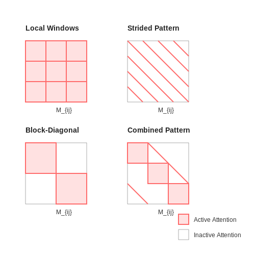
Fixed sparse patterns like block-sparse attention or stride patterns reduce the quadratic complexity:
The sparsity mask M enforces:
Common variants include:
- Local windows (neighborhood attention)
- Strided patterns (every k-th token)
- Block-diagonal structures
Kernel Fusion and Operator Optimization
Transformer throughput benefits from fused operations:
# Before fusion (separate ops)
q = torch.matmul(x, W_q)
k = torch.matmul(x, W_k)
v = torch.matmul(x, W_v)

# After fusion (single op)
qkv = torch.matmul(x, torch.cat([W_q, W_k, W_v], dim=-1))
q, k, v = torch.split(qkv, d_model, dim=-1)
Additional optimizations include:
- Activation checkpointing (recompute instead of store)
- Gradient accumulation for larger effective batches
- Efficient CUDA kernels for rotary position embeddings
Model Parallelism Strategies
For very large models, computation is distributed via:
| Strategy | Communication Pattern | Best For |
|---|---|---|
| Tensor Parallelism | All-reduce within layers | Single-node multi-GPU |
| Pipeline Parallelism | Point-to-point between stages | Multi-node scenarios |
| Expert Parallelism (MoE) | All-to-all for expert routing | Sparse models |
The communication overhead for tensor parallelism in a linear layer is:
where α is latency and β is bandwidth, requiring careful balancing of partition sizes.
4. Sparse and Efficient Attention Mechanisms
4.1 Sparse and Efficient Attention Mechanisms
Computational Challenges of Dense Attention
The standard self-attention mechanism in transformers computes pairwise interactions between all tokens in a sequence, resulting in a computational complexity of
Sparse Attention Patterns
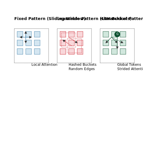
Sparse attention mechanisms reduce computational overhead by restricting the attention field through predefined or learned patterns. Three principal approaches dominate current research:
- Fixed Patterns: Implement windowed attention (e.g., local neighborhoods) or strided attention (e.g., every k-th token). The Longformer employs a combination of sliding window attention and global attention on task-specific tokens.
- Learnable Patterns: The Reformer's locality-sensitive hashing (LSH) attention groups similar queries and keys into buckets, reducing the effective sequence length for attention computation.
- Hierarchical Patterns: The BigBird model combines random attention, windowed attention, and global attention to maintain theoretical expressiveness while reducing complexity to $$ O(N) $$.
Low-Rank Approximation Methods
Alternative approaches approximate the full attention matrix using low-rank decompositions. The Linformer projects keys and values to a lower-dimensional space (k ≪ N) through learned linear transformations:
where E ∈ ℝN×k and F ∈ ℝk×N are projection matrices. This reduces memory usage from O(N2) to O(Nk) while preserving performance on many tasks.
Memory-Efficient Implementations
Modern libraries employ several optimization strategies:
- FlashAttention: Leverages tiling to keep attention computations in SRAM, reducing memory reads/writes through fused kernel operations. Achieves 2-4× speedup on GPUs.
- Block-Sparse Attention: Divides the attention matrix into blocks and applies sparsity at the block level, enabling efficient utilization of tensor cores in modern accelerators.
- Gradient Checkpointing: Selectively recomputes attention activations during backpropagation to trade computation for memory savings.
Theoretical Trade-offs
The sparse vs. dense attention trade-off can be formalized through the universal approximation theorem for transformers. Let Asparse be a sparse attention pattern with maximum path length l between any two tokens. Then:
This explains why models like the Sparse Transformer require deeper architectures to maintain representational capacity when using constrained attention patterns.
Practical Considerations
When implementing sparse attention in frameworks like PyTorch:
class BlockSparseAttention(nn.Module):
    def __init__(self, block_size, sparsity_ratio):
        super().__init__()
        self.block_size = block_size
        self.sparsity_mask = self._generate_mask(sparsity_ratio)

    def forward(self, Q, K, V):
        # Reshape into blocks
        Q_blocks = Q.view(-1, self.block_size, Q.size(-1))
        K_blocks = K.view(-1, self.block_size, K.size(-1))

        # Compute block-sparse attention
        attn = torch.einsum('bqd,bkd->bqk', Q_blocks, K_blocks)
        attn = attn.masked_fill(~self.sparsity_mask, float('-inf'))
        return torch.matmul(F.softmax(attn, dim=-1), V)
Key hyperparameters include block size (typically 32-128 tokens) and sparsity ratio (often 0.1-0.3). The optimal configuration depends on the task's locality requirements and hardware constraints.
4.2 Transformer Variants (BERT, GPT, etc.)
Architectural Divergence in Transformer Variants
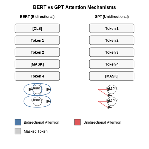
The original Transformer architecture introduced by Vaswani et al. (2017) serves as the foundation for modern variants, but key modifications distinguish BERT, GPT, and other derivatives. The primary divergence lies in the self-attention mechanism and training objectives. While the vanilla Transformer uses bidirectional self-attention for sequence transduction tasks, BERT employs masked language modeling (MLM) and next sentence prediction (NSP), whereas GPT relies exclusively on unidirectional attention with autoregressive language modeling.
Here, U(1,n) represents uniform sampling over token positions, and x_{\setminus i} denotes the sequence with the i-th token masked. This contrasts with GPT's autoregressive objective:
BERT: Bidirectional Encoder Representations
BERT's architecture consists of stacked Transformer encoder blocks with two critical innovations: dynamic masking and sentence-level pretraining. Unlike the original Transformer, BERT processes input tokens in parallel through multiple layers of bidirectional self-attention, allowing each token to attend to all other tokens in the sequence. The model's pretraining involves predicting randomly masked tokens (15% of input) and determining whether two sentences follow each other in the original text.
Key Architectural Details
- Token Embeddings: WordPiece tokenization with 30,000 vocabulary size
- Positional Encoding: Learned embeddings instead of sinusoidal functions
- Attention Heads: 12-16 heads with 768-1024 hidden dimensions
- Layer Normalization: Applied before (pre-LN) rather than after (post-LN) residual connections
GPT: Autoregressive Decoder Architecture
The GPT family (Generative Pretrained Transformer) exclusively uses Transformer decoder blocks with masked self-attention. The key constraint is the causal attention mask, which prevents tokens from attending to future positions during training. This architecture enables powerful text generation through next-token prediction but lacks bidirectional context understanding.
where M is a lower triangular mask matrix with −∞ in positions i > j. GPT-3 scaled this approach to 175 billion parameters using:
- Sparse attention patterns (alternating dense and locally banded attention)
- Learned positional embeddings with context windows up to 8,192 tokens
- Adaptive computation time for different layers
Hybrid Architectures and Recent Variants
Recent models like T5 (Text-to-Text Transfer Transformer) and Switch Transformers combine aspects of both architectures. T5 reformulates all NLP tasks into a text-to-text format using a unified encoder-decoder structure, while Switch Transformers employ mixture-of-experts routing:
where G(x) is a gating network that routes inputs to expert networks E_i. This allows for parameter-efficient scaling beyond 1 trillion parameters while maintaining computational feasibility through conditional execution.
4.3 Cross-Attention in Encoder-Decoder Models
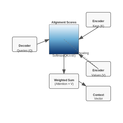
Cross-attention is the mechanism that enables the decoder in a transformer to dynamically focus on relevant parts of the encoder's output. Unlike self-attention, where queries, keys, and values originate from the same sequence, cross-attention computes attention scores between the decoder's queries and the encoder's keys and values. This allows the decoder to condition its output on the encoded representation of the input sequence.
Mathematical Formulation
Given the encoder's output E ∈ ℝn×d (where n is the input sequence length and d is the embedding dimension) and the decoder's hidden state H ∈ ℝm×d (where m is the target sequence length), cross-attention computes:
Here:
- Queries (Q) are derived from the decoder's hidden state: Q = HWQ.
- Keys (K) and Values (V) come from the encoder's output: K = EWK, V = EWV.
The scaling factor √dk stabilizes gradients by preventing dot products from growing too large in magnitude.
Mechanism and Interpretation
Cross-attention operates in three steps:
- Alignment: Computes attention scores between decoder queries and encoder keys, identifying which encoder tokens are most relevant for the current decoder step.
- Weighted Sum: Uses these scores to compute a context vector as a weighted sum of encoder values.
- Integration: Combines the context vector with the decoder's current state to produce the next output.
This mechanism is particularly powerful in sequence-to-sequence tasks like machine translation, where the decoder must align target words with relevant source words dynamically.
Practical Considerations
In autoregressive decoding, cross-attention is computed sequentially for each decoder step. To maintain causality, the decoder uses masked self-attention for its own states while applying cross-attention to the full encoder output. Modern implementations often optimize this using key-value caching to avoid recomputing encoder projections at every step.
Variants like multi-head cross-attention split the computation into parallel heads, allowing the model to attend to different encoder subspaces simultaneously. For example, in a translation task, one head might focus on lexical meaning while another captures syntactic structure.
Visualization of Cross-Attention
A typical cross-attention heatmap shows strong diagonal alignment in tasks like translation, where word order is roughly preserved. However, it can also reveal non-local dependencies—for instance, attending to a verb's subject earlier in the sentence when generating an inflection.
5. Key Research Papers on Transformers
5.1 Key Research Papers on Transformers
- 11.7. The Transformer Architecture — Dive into Deep Learning 1. ... - D2L — 11.7.5. Decoder¶. As shown in Fig. 11.7.1, the Transformer decoder is composed of multiple identical layers.Each layer is implemented in the following TransformerDecoderBlock class, which contains three sublayers: decoder self-attention, encoder-decoder attention, and positionwise feed-forward networks. These sublayers employ a residual connection around them followed by layer normalization.
- Vision transformers inference acceleration based on adaptive layer ... — In this section, we provide an overview of the key modules of the standard Vision Transformers (ViT). The standard Transformer block consists of two primary sub-layers: multihead self-attention (MSA) and a Feed-Forward-Network (FFN). Additionally, each sub-layer is equipped with a residual connection and layer normalization [31]. These main ...
- Power electronic transformers: A review - ScienceDirect — The power transformers are the key components of the isolated DC-DC power converters with high voltage gain which has become a popular topic in recent years [1], [7], [10], [11].In the isolated DC-DC converter applications, power transformers have three main tasks [12], [13], [14].First one is to ensure galvanic insulation through magnetic coupling between the low voltage and high voltage side.
- 9 Transformers - 6.390 - Intro to Machine Learning — In practice, this addition occurs at the very first layer of the transformer stack, and all subsequent layers operate on position-aware representations. This is a key design choice that allows transformers to work effectively with sequences of text, audio, or even image patches (as in Vision Transformers). 9.5.2 Causal Self-attention
- PDF Block-Recurrent Transformers - NeurIPS — also operates on blocks of tokens; each layer takes, as input, the outputs of the same layer from the previous block. 3 Method The Block-Recurrent Transformer is based on sliding-window attention [33], which is an extension of ideas from Transformer-XL [34]. A long document, such as a book, consists of a sequence of tokens. Due to memory ...
- The Explainability of Transformers: Current Status and Directions - MDPI — An increasing demand for model explainability has accompanied the widespread adoption of transformers in various fields of applications. In this paper, we conduct a survey of the existing literature on the explainability of transformers. We provide a taxonomy of methods based on the combination of transformer components that are leveraged to arrive at the explanation. For each method, we ...
- Few-Shot Learning with Semi-Supervised Transformers for Electronic ... — Following the recent advances on transformers and BERT-based models, we also plan on exploring different architecture possibilities for our transformer network such as Electra (Clark et al., 2020), XLNet (Yang et al., 2019b), or RoBERTa (Liu et al., 2019) to name a few. Additionally, we will investigate the benefits of using a transformer-based ...
- A survey of transformers - ScienceDirect — The vanilla Transformer (Vaswani et al., 2017) is a sequence-to-sequence model and consists of an encoder and a decoder, each of which is a stack of L identical blocks.Each encoder block is mainly composed of a multi-head self-attention module and a position-wise feed-forward network (FFN). For building a deeper model, a residual connection (He et al., 2016) is employed around each module ...
- A Survey of Transformers - arXiv.org — In Transformer, there are three types of attention in terms of the source of queries and key-value pairs: •Self-attention. In Transformer encoder, we set Q = K = V = X in Eq. (2), where X is the outputs of the previous layer. •Masked Self-attention. In the Transformer decoder, the self-attention is restricted such that
- Decoupling Knowledge and Reasoning in Transformers: A Modular ... — Our modular Transformer block replaces the standard Feed-Forward Network (FFN) with a cross-attention layer that attends to E 𝐸 E italic_E. This design choice is motivated by the hypothesis that FFNs in standard Transformers implicitly perform a form of context-dependent knowledge retrieval.
5.2 Recommended Books and Tutorials
- PDF Transformers for Machine Learning; A Deep Dive — 6.4 MULTIMODAL AND MULTITASKING TRANSFORMER 166 6.4.1 Vision-and-LanguageBERT(VilBERT) 167 6.4.2 UnifiedTransformer(UniT) 168 6.5 VIDEO PROCESSING WITH TIMESFORMER 169 6.5.1 PatchEmbeddings 169 6.5.2 Self-Attention 170 6.5.2.1 Spatiotemporalself-attention 171 6.5.2.2 Spatiotemporalattentionblocks 171 6.6 GRAPH TRANSFORMERS 172
- 11.7. The Transformer Architecture — Dive into Deep Learning 1. ... - D2L — 11.7.5. Decoder¶. As shown in Fig. 11.7.1, the Transformer decoder is composed of multiple identical layers.Each layer is implemented in the following TransformerDecoderBlock class, which contains three sublayers: decoder self-attention, encoder-decoder attention, and positionwise feed-forward networks. These sublayers employ a residual connection around them followed by layer normalization.
- PDF Transformers for Vision - Department of Computer Science — Transformer block •A Transformer is a sequence of transformer blocks •Vaswani et al.: •12 blocks, 512 embedding dimension, 6 attention heads •Multi-Head Attention: introduced before •Add & Norm: residual connection followed by layer normalization •Feedforward (Multi-layer perceptron): two linear layers with ReLUsin between, applied
- Transformer and Inductor Design Handbook Colonel T Mclyman — Ask the publishers to restore access to 500,000+ books. An icon used to represent a menu that can be toggled by interacting with this icon. A line drawing of the Internet Archive headquarters building façade. ... transformer-and-inductor-design-handbook-colonel-t-mclyman Identifier-ark ark:/13960/s2mnsktwgrp Ocr tesseract 5.2.0-1-gc42a Ocr ...
- 9 Transformers - 6.390 - Intro to Machine Learning — Specifically, each block consists of two primary sub-layers: an attention layer Section 9.4 and a feed-forward network (or multi-layer perceptron) Chapter 6. Attention layers mix information across different positions (or "chunks") in the sequence, allowing the model to effectively capture dependencies regardless of distance.
- Book NLP with Transformers: Fundamentals and Core Applications by ... — A basic understanding of Python and Machine Learning is recommended, but no prior experience with transformers is required. The book starts with foundational concepts and gradually builds up to more advanced topics, making it accessible to both beginners and experienced practitioners looking to deepen their knowledge of NLP with transformers.
- PDF Transformer Engineering: Design, Technology, and Diagnostics — engineers in the transformer industry and the student community. A few improvements have been incorporated in the other chapters as well. Understanding the basics of electromagnetic fields is an essential prerequisite for doing advanced computations. Chapter 12 explains the field theory relevant to transformer engineering in a simple manner.
- Transformers for machine learning. A deep dive. - Anna's Archive — Key Features: A comprehensive reference book for detailed explanations for every algorithm and techniques related to the transformers. 60+ transformer architectures covered in a comprehensive manner. A book for understanding how to apply the transformer techniques in speech, text, time series, and computer vision.
- PDF The Little Book of Deep Learning - Fleuret — Instead of trying to be exhaustive, this little book is limited to the background necessary to under-stand a few important models. This proved to be a popular approach, resulting in more than 500,000 downloads of the PDF file in the 12 months following its announcement on Twitter. If you did not get this book from its official URL
- Deep Learning — The online version of the book is now complete and will remain available online for free. The deep learning textbook can now be ordered on Amazon . For up to date announcements, join our mailing list .
5.3 Open-Source Implementations and Tools
- PDF Segmenter: Transformer for Semantic Segmentation - CVF Open Access — A transformer [50] encoder composed of Llayers is ap-plied to the sequence of tokens z 0 to generate a sequence of contextualized encodings z L ∈RN×D. A transformer layer consists of a multi-headed self-attention (MSA) block fol-lowed by a point-wise MLP block of two layers with layer norm (LN) applied before every block and residual connec-
- 11.7. The Transformer Architecture — Dive into Deep Learning 1. ... - D2L — 11.7.5. Decoder¶. As shown in Fig. 11.7.1, the Transformer decoder is composed of multiple identical layers.Each layer is implemented in the following TransformerDecoderBlock class, which contains three sublayers: decoder self-attention, encoder-decoder attention, and positionwise feed-forward networks. These sublayers employ a residual connection around them followed by layer normalization.
- Multi-task Active Learning for Pre-trained Transformer-based Models — The input text, as encoded by the shared 8 layers, e 1: 8 S , is passed through the shared and non-shared 4-layer modules, e 8: 12 S and e 8: 12 U i , respectively. The task classifiers are then fed with the output of the cross-task layers combined with the output of their task-specific layers, following the gating mechanism of Rotman and ...
- Regularizing transformers with deep probabilistic layers — It is composed of a first step with the computation of the input sentence embeddings, then a pile of transformer encoder layers, and then, if it is necessary, we can apply any task-specific layer on top. Each encoder layer consists of two blocks, a multi-head self-attention mechanism, and a feed-forward network, with a normalization following them.
- GitHub - NVIDIA/FasterTransformer: Transformer related optimization ... — Fund open source developers The ReadME Project. GitHub community articles Repositories. Topics ... FasterTransformer implements a highly optimized transformer layer for both the encoder and decoder for inference. On Volta, Turing and Ampere GPUs, the computing power of Tensor Cores are used automatically when the precision of the data and ...
- What Is Next for LLMs? Next-Generation AI Computing Hardware Using ... — Figure 13: Magnetic tunnel junctions for memory applications. a, A magnetic tunnel junction consists of two ferromagnetic layers (grey) separated by an insulating layer (blue) with the magnetization of one layer fixed and that of the other either parallel (low resistance) or antiparallel (high resistance) to it. The labels '1' and '0 ...
- Efficient Automated Circuit Discovery in Transformers using Contextual ... — This task was performed on a 4-layer attention-only transformer trained on natural language and Python code (attn-only-4l) released with the TransformerLens library for the express purpose of facilitating mechanistic interpretability research. Another complication is that the toy model only guesses the correct token between 60 and 65 percent of ...
- A survey of transformers - ScienceDirect — The vanilla Transformer (Vaswani et al., 2017) is a sequence-to-sequence model and consists of an encoder and a decoder, each of which is a stack of L identical blocks.Each encoder block is mainly composed of a multi-head self-attention module and a position-wise feed-forward network (FFN). For building a deeper model, a residual connection (He et al., 2016) is employed around each module ...
- Transformers in Time-Series Analysis: A Tutorial — Transformer architectures have widespread applications, particularly in Natural Language Processing and Computer Vision. Recently, Transformers have been employed in various aspects of time-series analysis. This tutorial provides an overview of the Transformer architecture, its applications, and a collection of examples from recent research in time-series analysis. We delve into an explanation ...
- Transformer Block Coupling and its Correlation with Generalization in LLMs — The results for ViTs demonstrate that stochastic depth encourages coupling during training (Figure LABEL:figure:coupling_vit b) and that coupling correlates with accuracy when fixing SD rate (Figure LABEL:figure:coupling_vit a). This finding suggests that coupling may provide new insight into stochastic depth's underlying mechanism, and that developing training methods to amplify coupling ...