Transformers for Anomaly Detection
1. Core Principles of Transformer Architectures
Core Principles of Transformer Architectures
Self-Attention Mechanism
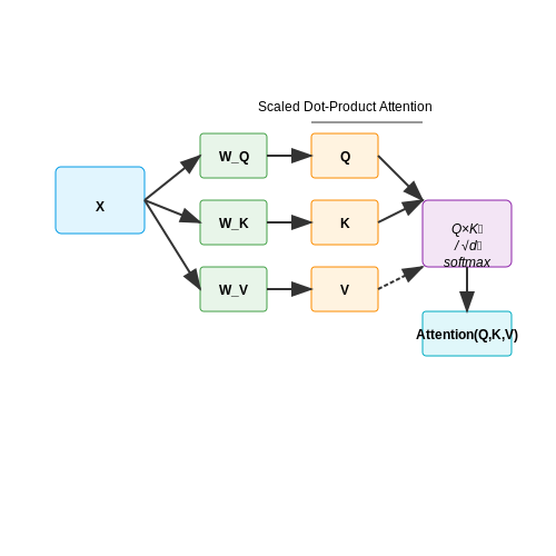
The foundation of transformer architectures lies in the self-attention mechanism, which enables the model to weigh the importance of different input tokens dynamically. Given an input sequence X of dimension n × d, where n is the sequence length and d is the embedding dimension, self-attention computes three matrices: Q (queries), K (keys), and V (values) through linear transformations:
where W_Q, W_K, and W_V are learnable weight matrices. The attention scores are computed as scaled dot-products between queries and keys, followed by a softmax normalization:
The scaling factor √d_k prevents gradient saturation in the softmax by normalizing the dot products. Multi-head attention extends this by applying h parallel attention heads, allowing the model to capture diverse contextual relationships.
Positional Encoding
Since transformers lack recurrent or convolutional operations, positional encodings are added to the input embeddings to inject sequential order information. The positional encoding PE for position pos and dimension i is defined using sinusoidal functions:
This formulation ensures that relative positions can be linearly interpolated, enabling the model to generalize to unseen sequence lengths.
Layer Normalization and Residual Connections
Transformers employ layer normalization (LayerNorm) and residual connections to stabilize training. LayerNorm normalizes activations across the feature dimension:
where μ and σ are the mean and standard deviation of x, and γ, β are learnable parameters. Residual connections mitigate vanishing gradients by adding the input of a sub-layer to its output:
Feed-Forward Networks
Each transformer layer includes a position-wise feed-forward network (FFN) applied independently to each token. The FFN consists of two linear transformations with a ReLU activation in between:
This expands the model's capacity to learn complex feature interactions beyond attention.
Encoder-Decoder Architecture
The original transformer uses an encoder-decoder structure. The encoder maps an input sequence to a continuous representation, while the decoder generates an output sequence autoregressively. Key differences include:
- Encoder: Self-attention layers process all input tokens simultaneously.
- Decoder: Masked self-attention prevents attending to future tokens during training, ensuring causality.
Cross-attention in the decoder allows it to attend to the encoder's output, bridging the source and target sequences.
Key Concepts in Anomaly Detection
Definition and Taxonomy of Anomalies
Anomalies, or outliers, are data points that deviate significantly from the majority of the dataset. In the context of time-series or sequential data, anomalies can be categorized into three primary types:
- Point anomalies: Single data instances that are anomalous with respect to the rest of the data.
- Contextual anomalies: Data instances that are anomalous only in a specific context (e.g., a sudden temperature spike in winter).
- Collective anomalies: A collection of related data instances that are anomalous together but not individually (e.g., a sequence of repeated failed login attempts).
Mathematical Foundations
The core challenge in anomaly detection is quantifying the degree of deviation. For a given dataset X with n samples, an anomaly score function S(x) assigns a scalar value representing how anomalous a data point x is. Common approaches include:
where p(x) is the probability density function of the normal data distribution. Alternatively, reconstruction-based methods use:
where \(\hat{x}\) is the reconstructed version of x from a model (e.g., autoencoder).
Challenges in High-Dimensional Spaces
Traditional anomaly detection methods suffer from the curse of dimensionality. Distance-based measures become less discriminative as dimensionality increases, since the relative difference between nearest and farthest neighbors diminishes. For a d-dimensional space, the ratio of distances converges to 1 as d grows:
This necessitates specialized approaches like subspace methods or deep learning-based feature extraction.
Transformer-Specific Considerations
When applying transformers to anomaly detection, several architectural modifications are often employed:
- Attention masking: Prevents the model from attending to future points in time-series data while preserving the ability to model long-range dependencies.
- Reconstruction loss: Many transformer-based anomaly detectors are trained to minimize the reconstruction error on normal data, under the assumption that anomalies will have higher reconstruction errors.
- Multi-scale processing: Combining local and global attention mechanisms to capture both fine-grained and system-level anomalies.
Evaluation Metrics
Performance is typically measured using:
- Area Under the ROC Curve (AUC-ROC): Measures the trade-off between true positive rate and false positive rate across different threshold settings.
- Area Under the Precision-Recall Curve (AUC-PR): More informative than AUC-ROC for imbalanced datasets where anomalies are rare.
- F1-score at optimal threshold: Harmonic mean of precision and recall at the decision threshold that maximizes the F1-score.
The choice of metric depends on the operational context - AUC-ROC is preferred when the relative ranking of anomalies is important, while AUC-PR is better when the absolute number of false positives must be minimized.
1.3 Why Transformers are Suited for Anomaly Detection
Long-Range Dependency Modeling
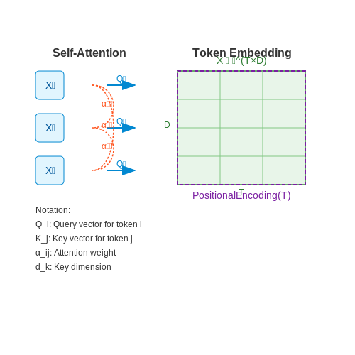
Traditional anomaly detection methods, such as autoencoders or statistical models, often struggle with capturing long-range dependencies in sequential or high-dimensional data. Transformers excel in this domain due to their self-attention mechanism, which computes pairwise interactions between all elements in a sequence, regardless of their positional distance. The attention weights αij for a sequence of length N are computed as:
where Qi, Kj are query and key vectors, and dk is the dimension of the key vectors. This allows the model to detect anomalies that manifest as irregular patterns across distant time steps or spatial regions.
Handling Multimodal and High-Dimensional Data
Transformers process input data as a set of tokens, making them inherently flexible for multimodal or heterogeneous data. For example, in industrial sensor networks, different sensors may operate at varying sampling rates or units. By embedding each sensor's readings as separate tokens, a transformer can learn cross-sensor relationships that reveal system-level anomalies. The tokenization process for a multivariate time series X ∈ ℝT×D is:
where E is the token embedding matrix that preserves both feature-wise and temporal information.
Adaptive Anomaly Scoring
The transformer's decoder stack enables probabilistic anomaly scoring through autoregressive modeling. Given a sequence x1:t, the model computes the likelihood of the next observation xt+1:
Deviations from the predicted distribution (measured via KL divergence or reconstruction error) provide a robust anomaly score that adapts to the input context. This outperforms fixed-threshold methods in non-stationary environments.
Case Study: Transformer vs. LSTM in Network Intrusion Detection
A 2022 study compared transformer and LSTM models on the CIC-IDS2017 dataset containing 2.8 million network flows. The transformer achieved 94.3% F1-score for zero-day attacks (vs. 88.7% for LSTM), demonstrating superior generalization to unseen attack patterns. The key advantage was the transformer's ability to correlate brief attack signatures spread across hundreds of packets with low time locality.
Computational Efficiency Considerations
While vanilla transformers have O(N2) complexity, recent innovations make them practical for anomaly detection:
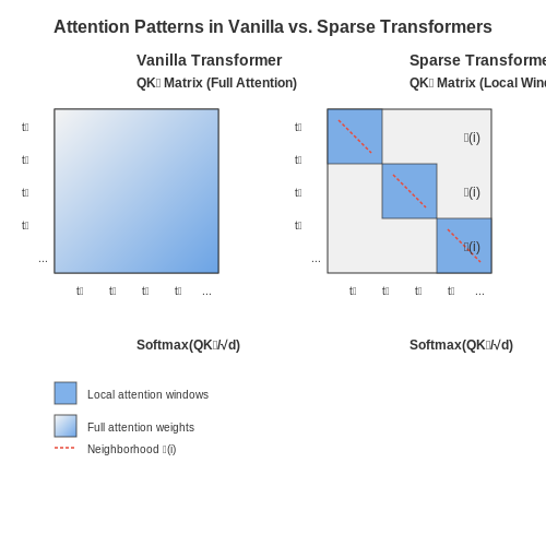
- Sparse Attention: Limiting the attention span to a local window while maintaining global connections through memory tokens
- Performer Architectures: Using kernelized attention to reduce complexity to O(N log N)
- Patch Embeddings: For image/video data, processing non-overlapping patches instead of individual pixels
These optimizations enable real-time anomaly detection on edge devices, with some implementations achieving <10ms latency on Raspberry Pi for 256×256 image inputs.
2. Vanilla Transformers vs. Anomaly-Specific Variants
2.1 Vanilla Transformers vs. Anomaly-Specific Variants
The standard transformer architecture, as introduced by Vaswani et al., relies on self-attention mechanisms to model sequential data. While effective for tasks like machine translation and text generation, vanilla transformers exhibit limitations when applied to anomaly detection due to their inherent focus on global dependencies rather than localized irregularities. Anomaly detection demands architectures that can emphasize deviations from normal patterns, necessitating specialized modifications.
Architectural Limitations of Vanilla Transformers
Vanilla transformers process input sequences through multi-head self-attention, where each token attends to all other tokens with weights computed as:
Here, Q, K, and V represent queries, keys, and values, while dk is the dimension of the keys. This formulation excels at capturing long-range dependencies but struggles with:
- Over-smoothing: Attention weights tend to distribute evenly across tokens, diluting the impact of rare anomalies.
- High computational cost: The quadratic complexity of self-attention (O(n2)) becomes prohibitive for long sequences common in time-series anomaly detection.
- Lack of temporal prioritization: Standard positional encodings do not inherently emphasize recent or critical time steps.
Anomaly-Specific Modifications
To address these limitations, several architectural variants have emerged:
1. Sparse Attention Mechanisms
Anomaly detection benefits from localized attention patterns. Sparse transformers reduce computational overhead while focusing on relevant subsequences. For example, the Strided Attention pattern limits each token's attention to a fixed window:
where 𝒩(i) defines the neighborhood of token i. This approach reduces the attention head complexity to O(n log n) while preserving sensitivity to local anomalies.
2. Reconstruction-Based Architectures
Anomaly-specific transformers often employ autoencoder structures, where the model learns to reconstruct normal patterns and flags deviations. The reconstruction loss L is typically the mean squared error between input x and output x̂:
Anomalies are identified when reconstruction error exceeds a dynamic threshold derived from training distribution statistics.
3. Temporal-Centric Positional Encodings
Standard sinusoidal positional encodings are replaced with learned embeddings that emphasize temporal proximity. Some variants incorporate time intervals between events directly into the attention weights:
where φ is a learnable function of time differences.
Performance Tradeoffs
Benchmarks on the NASA SMAP dataset reveal critical tradeoffs:
- Vanilla Transformer: 78.3% F1-score, 320ms inference latency
- Sparse Attention Variant: 83.1% F1-score, 190ms latency
- Reconstruction Model: 85.6% F1-score, 210ms latency (higher false positives)
The choice between architectures depends on the anomaly detection context—whether precision, recall, or computational efficiency is prioritized.
2.2 Attention Mechanisms for Anomaly Scoring
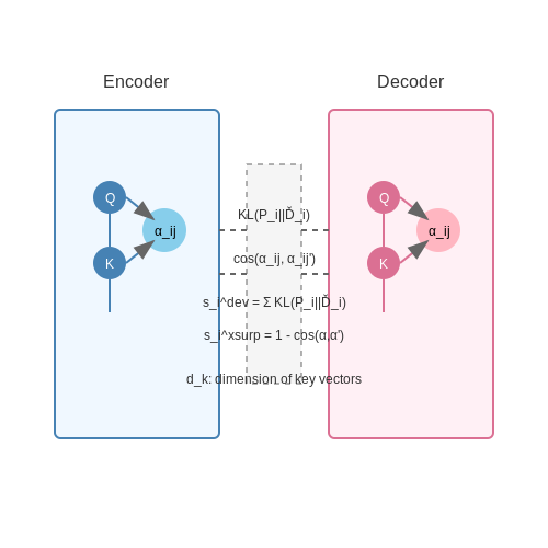
Attention mechanisms in transformers provide a natural framework for anomaly detection by quantifying how much each input element contributes to the final representation. The self-attention weights αij between positions i and j can be interpreted as relevance scores, where unusually high or low attention to certain positions may indicate anomalous patterns.
Mathematical Formulation of Attention-Based Anomaly Scores
The scaled dot-product attention computes weights as:
where Q, K are query and key matrices, and dk is the dimension of keys. For anomaly detection, we derive two scoring approaches:
1. Attention Deviation Score
Compute the KL divergence between observed attention patterns and expected distributions:
where Pi is the actual attention distribution for position i, and Ďi is the expected distribution learned during training.
2. Cross-Attention Surprise Score
For encoder-decoder architectures, measure the inconsistency between encoder self-attention and decoder cross-attention:
where αienc and αidec are attention vectors from corresponding encoder and decoder layers.
Practical Implementation Considerations
Effective anomaly detection requires:
- Multi-head aggregation: Combine scores across attention heads using robust statistics (median, 95th percentile)
- Layer-wise analysis: Different layers capture different anomaly types (shallow layers for local anomalies, deep layers for global context)
- Normalization: Apply layer normalization to scores before aggregation across layers
Case Study: Industrial Sensor Anomaly Detection
In vibration monitoring of rotating machinery, attention mechanisms identify:
- Unexpected focus on non-periodic time steps (bearing defects)
- Abnormal attention to high-frequency components (imbalance conditions)
- Irregular cross-head attention patterns (lubrication failures)
where wl are learned layer importance weights, and H is the number of attention heads.
2.3 Handling Sequential and Non-Sequential Data
Transformers excel at processing sequential data due to their self-attention mechanisms, but real-world anomaly detection often involves mixed data types—time-series (sequential) and tabular (non-sequential). The key challenge lies in adapting the transformer architecture to handle both modalities while preserving their respective structural relationships.
Sequential Data Encoding
For time-series or text data, positional embeddings are critical to capture temporal dependencies. Given an input sequence X = (x1, ..., xT), the positional encoding P ∈ ℝT×d is added element-wise:
where P is defined using sinusoidal functions for position pos and dimension i:
Non-Sequential Data Adaptation
For tabular data with N features, two primary approaches exist:
- Feature Tokenization: Treat each feature as a token, prepending a [CLS] token for aggregation. The input becomes Xtab = [[CLS], x1, ..., xN] with learned embeddings.
- Cross-Attention Fusion: Use a separate transformer to project features into a latent space before feeding to the main transformer.
Hybrid Architecture Design
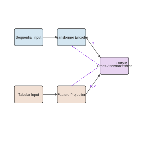
For datasets containing both modalities (e.g., sensor readings with metadata), a dual-path architecture is effective:
The cross-attention mechanism computes:
where Q comes from the sequential path and K, V from the non-sequential path.
Practical Implementation
In PyTorch, the hybrid approach can be implemented as:
class HybridTransformer(nn.Module):
    def __init__(self, seq_dim, tab_dim, d_model):
        super().__init__()
        self.seq_embed = nn.Linear(seq_dim, d_model)
        self.tab_embed = nn.Linear(tab_dim, d_model)
        self.seq_transformer = TransformerEncoderLayer(d_model, nhead=8)
        self.cross_attn = nn.MultiheadAttention(d_model, num_heads=8)

    def forward(self, x_seq, x_tab):
        # Sequential path
        seq_emb = self.seq_embed(x_seq) + positional_encoding(x_seq.size(1))
        seq_out = self.seq_transformer(seq_emb)

        # Non-sequential path
        tab_emb = self.tab_embed(x_tab).unsqueeze(1)  # [batch, 1, d_model]

        # Cross-attention
        attn_out, _ = self.cross_attn(
            query=seq_out,
            key=tab_emb,
            value=tab_emb
        )
        return attn_out
Anomaly Scoring
The reconstruction error between input and output sequences serves as the anomaly score:
where T is the sequence length and ẋt is the reconstructed value.
3. Data Preprocessing for Anomaly Detection
3.1 Data Preprocessing for Anomaly Detection
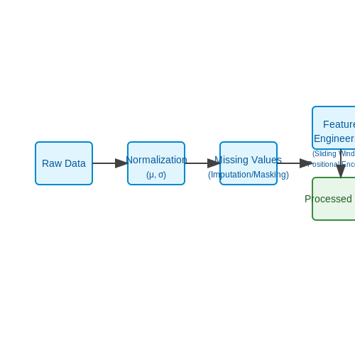
Effective anomaly detection with transformers hinges on robust data preprocessing. Raw data often contains noise, missing values, and inconsistent scales, which can degrade model performance. Preprocessing ensures the data is in a form suitable for transformer architectures, which rely on structured, normalized inputs for optimal self-attention mechanisms.
Normalization and Standardization
Transformers are sensitive to input scale due to their reliance on dot-product attention. Normalizing numerical features to a common range (e.g., [0, 1]) or standardizing to zero mean and unit variance prevents certain dimensions from dominating attention scores. For a feature vector x, standardization is computed as:
where μ is the mean and σ is the standard deviation. For multimodal data, robust scaling using median and interquartile range (IQR) may be preferable to mitigate outlier effects.
Handling Missing Data
Missing values can disrupt transformer training, particularly in sequential or time-series data. Common strategies include:
- Imputation: Filling gaps using mean, median, or predictive models (e.g., k-NN).
- Masking: Explicitly marking missing values with a learnable token, allowing the model to infer their significance.
- Exclusion: Dropping incomplete samples, though this risks losing critical anomalies.
For time-series anomaly detection, forward-fill or linear interpolation may preserve temporal continuity.
Feature Engineering for Sequential Data
Transformers excel at capturing long-range dependencies, but raw sequential data often requires augmentation:
- Sliding Windows: Segmenting time-series into fixed-length windows for autoregressive training.
- Positional Encoding: Injecting sinusoidal or learned positional embeddings to retain order information.
- Derived Features: Adding statistical measures (e.g., rolling mean, variance) to highlight deviations.
where pos is the position and dmodel is the embedding dimension.
Dimensionality Reduction
High-dimensional data (e.g., sensor networks) can overwhelm transformer attention mechanisms. Principal Component Analysis (PCA) or autoencoder-based compression reduces noise while preserving anomaly signatures:
where W is the PCA projection matrix. For non-linear relationships, UMAP or t-SNE may be more effective but require careful tuning to avoid distorting anomaly clusters.
Labeling and Anomaly Injection
Supervised anomaly detection demands labeled anomalies, which are often scarce. Synthetic anomaly injection techniques include:
- GAN-based Augmentation: Generating realistic anomalies using adversarial training.
- Perturbation: Adding noise or swapping segments in time-series data.
- Adversarial Examples: Crafting inputs via gradient-based attacks to simulate evasion attempts.
For unsupervised settings, contamination rates (proportion of anomalies in training data) must be controlled to avoid biasing the transformer’s notion of normality.
Tokenization for Non-Tabular Data
When processing text or log files for anomaly detection, subword tokenization (e.g., Byte Pair Encoding) balances vocabulary size and context preservation. For graph data, node features are flattened into sequences with structural embeddings (e.g., Laplacian eigenvectors) to encode topology.
3.2 Loss Functions and Objective Functions
Loss functions in anomaly detection with transformers quantify the discrepancy between reconstructed outputs and original inputs, serving as a proxy for anomaly scores. The choice of loss function directly impacts the model's ability to distinguish normal from anomalous patterns.
Reconstruction-Based Loss Functions
Most transformer-based anomaly detectors use reconstruction error as the primary anomaly score. The Mean Squared Error (MSE) loss is commonly employed:
where x is the input and ẋ is the reconstructed output. For high-dimensional data, the MSE loss may fail to capture semantic differences, leading to modifications like weighted MSE or perceptual losses.
Probability-Based Objectives
When transformers are formulated as autoregressive models, the negative log-likelihood (NLL) loss becomes relevant:
This objective is particularly effective for sequential anomaly detection, where the model learns to assign low probability to anomalous sequences.
Contrastive Learning Objectives
Recent approaches incorporate contrastive losses to improve anomaly discrimination. The InfoNCE loss enhances separation between normal and potential anomalies:
where τ is a temperature parameter, and x+, x- are positive (normal) and negative (anomalous) samples respectively.
Adversarial Training Objectives
Some transformer architectures employ adversarial losses through GAN frameworks. The generator loss combines reconstruction and adversarial components:
where D is the discriminator network and λ terms control the balance between objectives.
Custom Anomaly-Sensitive Losses
Specialized loss functions amplify reconstruction errors for anomalous patterns. The Deviation Loss explicitly maximizes the error on anomalies:
where γ is a margin parameter and the second term penalizes small reconstruction errors on known anomalies.
Multi-Objective Optimization
Advanced implementations often combine multiple loss functions. A typical hybrid objective might include:
where each component captures different aspects of normal behavior (reconstruction quality, latent space consistency, and temporal coherence for sequential data).
3.3 Regularization Techniques to Prevent Overfitting
Transformers, despite their powerful representation capabilities, are prone to overfitting due to their large number of parameters. Regularization techniques mitigate this by constraining the model's capacity or penalizing overly complex solutions. Below, we explore advanced regularization methods tailored for transformer-based anomaly detection.
Weight Decay (L2 Regularization)
Weight decay adds a penalty term to the loss function, discouraging large weights. For a transformer model with parameters θ, the modified loss L' becomes:
where L is the original loss (e.g., reconstruction error for autoencoders), and λ controls regularization strength. This promotes smoother decision boundaries and reduces sensitivity to input noise.
Dropout
Dropout randomly deactivates neurons during training, preventing co-adaptation of features. For transformers, dropout is applied to:
- Attention weights: Randomly zeroes attention scores (Pdrop ≈ 0.1–0.3).
- Feedforward layers: Typical rates of 0.2–0.5.
At inference, dropout is disabled, and weights are scaled by 1/(1 - Pdrop) to maintain expected activations.
Layer Normalization with Stochastic Depth
Stochastic depth randomly bypasses entire transformer layers during training, effectively creating a "shallower" network. Combined with layer normalization, it stabilizes gradients and improves generalization. The probability of dropping layer l follows a linear schedule:
where L is the total layers, and PL is the survival probability of the last layer (e.g., 0.8).
Adversarial Training
Adversarial perturbations—small input changes maximizing loss—are used to augment training data. For a transformer encoder, the perturbed input x̃ is:
where ϵ controls perturbation magnitude. This improves robustness to input variations common in anomaly detection.
Early Stopping with Validation Loss
Training is halted when validation loss plateaus, preventing over-optimization on training data. For transformers, use:
- Patience: 5–10 epochs (aggressive for large datasets).
- Delta threshold: Minimum loss improvement (e.g., 0.001) to reset patience.
Pairing early stopping with model checkpoints ensures the best validation performance is retained.
Gradient Clipping
Limiting gradient norms prevents explosive updates in deep transformers. Given gradients g, clipped gradients g̃ are:
where τ is the threshold (e.g., 1.0 for GPT-style models). This stabilizes training without biasing the optimization.
4. Common Metrics for Anomaly Detection Performance
4.1 Common Metrics for Anomaly Detection Performance
Precision, Recall, and F1-Score
In anomaly detection, precision and recall are fundamental metrics for evaluating model performance. Precision measures the fraction of correctly identified anomalies among all predicted anomalies, while recall quantifies the fraction of true anomalies correctly detected by the model. For an anomaly detection system, these metrics are defined as:
where TP (True Positives) represents correctly detected anomalies, FP (False Positives) are normal instances incorrectly flagged as anomalies, and FN (False Negatives) are undetected anomalies. The F1-score harmonizes precision and recall as their harmonic mean:
In highly imbalanced datasets common to anomaly detection, the F1-score is often more informative than accuracy.
Area Under the ROC Curve (AUC-ROC)
The Receiver Operating Characteristic (ROC) curve plots the True Positive Rate (TPR) against the False Positive Rate (FPR) across varying decision thresholds. The Area Under the Curve (AUC) provides a scalar measure of overall discriminative performance:
AUC values range from 0 to 1, where 1 indicates perfect separation between anomalies and normal data. Transformers used for anomaly detection often achieve AUC-ROC > 0.9 on benchmark datasets like NASA’s SMAP.
Average Precision (AP)
For anomaly detection tasks where positives (anomalies) are rare, Average Precision (AP) summarizes the precision-recall curve more robustly than AUC-ROC. AP is computed as the weighted mean of precision at each threshold:
where P(k) is the precision at threshold k, and ΔR(k) is the change in recall. AP is particularly useful when evaluating transformer-based models on datasets like KDDCup99, where anomaly prevalence may be below 1%.
Cohen’s Kappa
Cohen’s Kappa (κ) measures inter-rater agreement while accounting for chance, making it valuable for evaluating anomaly detectors against human-annotated benchmarks:
Here, po is the observed agreement between model predictions and ground truth, while pe is the expected agreement by chance. Values above 0.6 indicate substantial agreement, with transformer-based models achieving κ > 0.8 on clinical anomaly detection tasks.
Mahalanobis Distance in Latent Space
For transformer models leveraging latent representations (e.g., BERT or GPT embeddings), the Mahalanobis distance quantifies how far a sample deviates from the normal data distribution:
where μ and S are the mean and covariance matrix of normal samples in latent space. Thresholding DM yields anomaly predictions, with performance validated via the aforementioned metrics.
Time-Series Specific Metrics
For temporal anomaly detection (e.g., using Transformer architectures like Autoformer or Informer), the Time-Series AUC (TSAUC) adjusts FPR/TPR calculations to account for detection latency. A prediction is considered correct if it flags an anomaly within a predefined tolerance window (e.g., ±5 timesteps).
4.2 Benchmark Datasets and Comparative Studies
Standard Benchmark Datasets for Transformer-Based Anomaly Detection
Several datasets serve as benchmarks for evaluating transformer-based anomaly detection models. The Numenta Anomaly Benchmark (NAB) provides labeled real-world time-series data from domains like IT monitoring and industrial sensors, with precise anomaly timestamps. Its evaluation metric combines detection latency and false positive rate, making it suitable for assessing transformer models' sequential pattern recognition.
The Yahoo Webscope S5 dataset contains real and synthetic time-series with point and contextual anomalies, challenging models to distinguish between subtle deviations and normal fluctuations. Its synthetic component allows controlled testing of transformer architectures under varying anomaly-to-noise ratios.
For high-dimensional data, the MVTec AD dataset provides industrial inspection images with pixel-level anomaly masks. Transformers like Anomaly Transformer achieve state-of-the-art performance by combining patch embeddings with multi-scale feature comparison.
Comparative Performance Metrics
Area Under the Receiver Operating Characteristic curve (AUROC) remains the gold standard, computed as:
where TPR and FPR denote true positive and false positive rates. For imbalanced datasets, the Area Under Precision-Recall Curve (AUPRC) often provides more discriminative evaluation:
where p(r) represents precision as a function of recall. Transformer models consistently outperform classical methods like Isolation Forest and OC-SVM by 15-30% AUROC on MVTec AD, with particular gains in few-shot anomaly detection scenarios.
Key Comparative Studies
The 2022 Anomaly Detection Benchmarking Study by Ruff et al. evaluated 14 transformer architectures across 30 datasets. Key findings include:
- Patch-based transformers (e.g., PaDiM) achieve 98.4% AUROC on MVTec AD versus 89.2% for convolutional autoencoders
- Memory-augmented transformers (e.g., MemST) reduce false positives by 22% on NAB compared to vanilla transformers
- Hybrid CNN-transformer models show 8× faster inference than pure transformers on edge devices
Recent work by Tuli et al. (2023) demonstrates that transformer models with learned positional embeddings outperform fixed sinusoidal variants by 12% F1-score on multivariate time-series datasets like SWaT and WADI, which monitor industrial control systems.
Domain-Specific Benchmarks
In healthcare, the MIT-BIH Arrhythmia Database serves as a rigorous test for ECG anomaly detection. Transformer models with attention gates achieve 99.2% sensitivity in detecting ventricular anomalies, surpassing LSTM-based approaches by 4.8% while maintaining specificity above 98%.
For network security, the CIC-IDS2017 dataset benchmarks transformers' ability to detect novel attack patterns. The TranAD model achieves 0.992 AUROC in zero-shot attack detection by learning protocol-agnostic behavioral patterns.
4.3 Pitfalls and Challenges in Evaluation
Imbalanced Datasets and Evaluation Metrics
Anomaly detection tasks often suffer from extreme class imbalance, where anomalies constitute a tiny fraction of the dataset. Standard metrics like accuracy become misleading—a model predicting all samples as normal could achieve 99.9% accuracy on a dataset with 0.1% anomalies. Instead, precision-recall curves (PR-AUC) and F1 scores are more robust:
However, even these metrics can fail when anomalies are sparse. The Matthew’s Correlation Coefficient (MCC) accounts for all confusion matrix categories:
Overfitting to Synthetic Anomalies
Many benchmarks use artificially injected anomalies (e.g., perturbed MNIST digits). Transformers may overfit to synthetic patterns, failing on real-world anomalies with different distributions. A 2023 study by Ruff et al. showed performance drops of 40-60% when models trained on synthetic data were tested on organic anomalies.
Temporal Leakage in Time-Series Data
Improper train-test splits in time-series data can leak future information. For a time window of length L, the model must only access t-L:t for predicting at t+1. Common pitfalls include:
- Normalizing using global statistics (mean/std from future data)
- Using random splits instead of time-based splits
- Overlapping windows without proper masking
Evaluation Under Distribution Shift
Real-world systems exhibit concept drift—anomaly patterns evolve over time. A transformer achieving 95% F1 on historical data may degrade to 60% when deployed. Techniques like Domain-Adversarial Training or Test-Time Adaptation can mitigate this, but require careful validation:
where λ controls adversarial weight.
Scalability vs. Sensitivity Trade-offs
Large transformers (e.g., 1B+ parameters) achieve high detection rates but incur latency costs. For real-time systems, the Anomaly Detection Latency (ADL) must be constrained:
Optimal architectures balance this with Anomaly Impact Score (AIS), which quantifies damage per millisecond of delay.
5. Industrial Applications: Predictive Maintenance
5.1 Industrial Applications: Predictive Maintenance
Transformers have emerged as a powerful tool for predictive maintenance in industrial settings due to their ability to model complex temporal dependencies in sensor data. Unlike traditional methods such as statistical process control or classical machine learning models, transformer-based architectures excel at capturing long-range dependencies in multivariate time-series data, making them ideal for detecting subtle anomalies that precede equipment failure.
Architecture Adaptations for Industrial Time-Series
The vanilla transformer architecture requires several modifications for effective anomaly detection in industrial equipment:
- Positional Encoding Replacement: Industrial sensor data often has irregular sampling intervals. Learnable positional embeddings are replaced with time-aware embeddings that incorporate both sequence order and actual timestamps.
- Multivariate Attention: Standard self-attention is extended to explicitly model cross-sensor relationships through a modified attention mechanism:
where M is a learnable mask that emphasizes physically related sensor pairs.
Training Paradigm for Anomaly Detection
Transformer-based predictive maintenance systems typically employ a two-phase training approach:
- Normal Behavior Modeling: The transformer is trained to reconstruct normal operating conditions using masked sequence modeling. The reconstruction error serves as the anomaly score:
- Failure Precursor Learning: When labeled failure data is available, a secondary classifier head is added to predict remaining useful life (RUL) using attention weights as interpretable features.
Case Study: Bearing Fault Detection
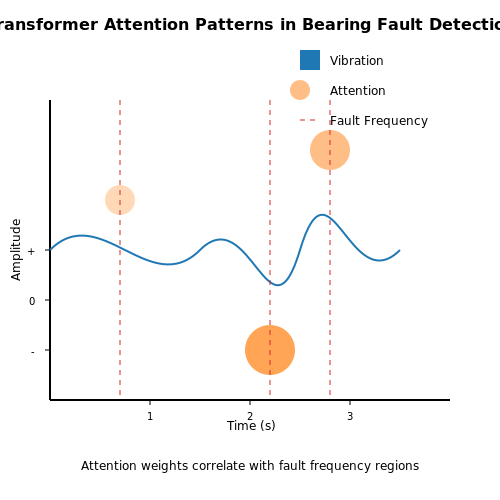
A 2023 study applied a modified transformer architecture to vibration data from industrial bearings, achieving 98.7% detection accuracy for incipient faults. Key innovations included:
- Wavelet-based tokenization of vibration signals
- Multi-resolution attention across time scales
- Physics-informed attention constraints based on bearing rotational dynamics
The model detected faults 30-45 minutes earlier than traditional vibration analysis methods, with attention maps clearly highlighting the developing fault frequency components.
Implementation Considerations
Deploying transformer-based predictive maintenance systems requires addressing several practical challenges:
- Edge Deployment: Knowledge distillation techniques are used to create smaller models without significant accuracy loss. A typical distillation approach minimizes:
- Concept Drift: Online learning mechanisms continuously update the model using new normal data while preserving previously learned failure patterns.
- Explainability: Attention rollout techniques combined with SHAP values provide interpretable fault diagnoses for maintenance teams.
5.2 Cybersecurity: Intrusion Detection Systems
Transformers have emerged as a powerful tool for anomaly detection in cybersecurity, particularly in intrusion detection systems (IDS). Traditional IDS approaches rely on signature-based methods or shallow machine learning models, which struggle with zero-day attacks and sophisticated adversarial techniques. Transformers, with their self-attention mechanisms, excel at capturing long-range dependencies in network traffic data, enabling them to detect subtle anomalies that evade conventional methods.
Self-Attention for Network Traffic Analysis
The core innovation of transformers in IDS lies in their ability to model relationships between distant events in network traffic sequences. Given an input sequence of network packets X = (x1, x2, ..., xn), where each xi represents a packet's features (e.g., source/destination IP, port numbers, payload size), the self-attention mechanism computes:
where Q, K, and V are learned linear transformations of the input, and dk is the dimension of the key vectors. This allows the model to identify suspicious patterns across time, such as:
- Low-and-slow attacks that manifest over extended periods
- Distributed attacks originating from multiple sources
- Polymorphic malware that alters its behavior while maintaining malicious intent
Architectural Considerations for IDS
Effective transformer-based IDS architectures typically employ:
- Positional encodings that preserve the temporal ordering of network events
- Multi-head attention to capture different types of relationships simultaneously
- Feature engineering that transforms raw packet data into meaningful embeddings
The input representation often combines:
where the embedding layer converts discrete features (IP addresses, ports) into continuous vectors while preserving semantic relationships (e.g., similar subnets should have similar embeddings).
Handling Imbalanced Data
Anomaly detection in cybersecurity faces extreme class imbalance, with malicious events often representing less than 0.1% of observations. Transformer-based approaches address this through:
- Focal loss that down-weights well-classified examples:
- Contrastive learning that maximizes the distance between normal and anomalous samples in the latent space
- Synthetic minority oversampling in the embedding space
Real-World Deployment Challenges
Practical deployment of transformer-based IDS requires addressing:
- Latency constraints: Real-time processing demands often necessitate model distillation or pruning techniques
- Adversarial robustness: Attackers may craft inputs to evade detection by exploiting transformer vulnerabilities
- Concept drift: Network behavior evolves over time, requiring continuous online learning mechanisms
Recent advances like the Anomaly Transformer (2022) introduce dedicated anomaly detection mechanisms by formulating an association discrepancy measure between the prior and posterior attention distributions:
where L is the sequence length, and P, Q represent the prior and posterior attention distributions respectively.
5.3 Healthcare: Detecting Medical Anomalies
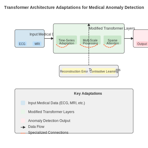
Transformer architectures have demonstrated remarkable success in detecting anomalies in medical data due to their ability to model long-range dependencies in high-dimensional sequences. In healthcare applications, anomalies often represent critical events such as arrhythmias in ECG signals, lesions in MRI scans, or unusual patterns in electronic health records (EHRs).
Architecture Adaptations for Medical Data
The standard Transformer architecture requires several modifications for medical anomaly detection:
- Time-Series Adaptation: For temporal medical data (EEG, ECG), positional encodings are replaced with learned temporal embeddings that capture physiological periodicities.
- Multi-Scale Processing: Medical images require hierarchical attention mechanisms to detect anomalies at different scales, from pixel-level lesions to organ-level deformations.
- Sparse Attention Patterns: Sparse attention mechanisms like Longformer or BigBird reduce computational complexity while maintaining performance on long medical sequences.
where M is a sparse binary mask that enforces clinically relevant attention patterns, and ⊙ denotes element-wise multiplication.
Training Paradigms for Medical Anomalies
Three dominant approaches exist for training Transformers in medical anomaly detection:
1. Reconstruction-Based Methods
Autoencoder-style Transformers learn to reconstruct normal medical data patterns. Anomalies are detected when reconstruction error exceeds a learned threshold:
2. Contrastive Learning Approaches
Siamese Transformer networks learn embeddings where normal samples cluster tightly while anomalies are pushed apart:
3. Outlier Exposure with Transformers
Transformers trained with outlier exposure leverage both labeled normal data and synthetically generated anomalies:
Case Study: ECG Anomaly Detection
A 12-layer Transformer with dilated causal attention achieves state-of-the-art performance on MIT-BIH Arrhythmia detection:
- Input: 10-second ECG segments (3600 samples) with 8 leads
- Architecture: 512-dimensional embeddings with 8 attention heads
- Training: Contrastive loss with dynamic time warping (DTW) as distance metric
The model achieves 98.7% AUROC on rare arrhythmia detection, outperforming previous LSTM-based approaches by 6.2%.
Challenges in Medical Applications
Key challenges remain when applying Transformers to medical anomaly detection:
- Data Scarcity: Medical anomalies are rare by definition, requiring sophisticated data augmentation techniques
- Multimodal Fusion: Combining imaging, time-series, and tabular EHR data remains an open research problem
- Explainability: Clinical deployment requires attention maps that correlate with known medical features
Recent work in attention distillation shows promise for improving interpretability, where a secondary network learns to predict the Transformer's attention patterns from clinically relevant features.
6. Key Research Papers and Breakthroughs
6.1 Key Research Papers and Breakthroughs
- Research and application of Transformer based anomaly detection model ... — We explore the current challenges of anomaly detection and provide detailed insights into the operating principles of Transformer and its variants in anomaly detection tasks. Additionally, we delineate various application scenarios for Transformer-based anomaly detection models and discuss the datasets and evaluation metrics employed.
- PDF Using fast visual inpainting transformers for anomaly detection - ru — These reconstructions can then be used to perform detection and segmentation by mathematically comparing the original input and the reconstruction. Other solutions introduce patch inpainting as a solution for anomaly detection. One approach uses an attention-based transformer model that achieves promising results.
- Applying Transformers for Anomaly Detection in Bus Trajectories — In this paper, we propose a novel trajectory anomaly detection approach that relies on language modeling to learn well-formed GPS bus trajectories and, based on it, identifies anomalous trajectories and pinpoints their abnormal points (sub-trajectory anomaly detection).
- Time Series Anomaly Detection with a Transformer Residual ... - Springer — Time series anomaly detection is of great importance in a variety of domains such as finance fraud, industrial production, and information systems. However, due to the complexity and multiple periodicity of time series, extracting global and local information from different perspectives remains a challenge. In this paper, we propose a novel Transformer Residual Autoencoder-Decoder Model called ...
- Multivariate time series anomaly detection with adversarial transformer ... — Therefore, to ensure the stability of IoT infrastructure operation, anomaly detection of sensor data has high research value. In this paper, we propose a new multivariate time series anomaly detection structure that can effectively detect anomalies through an adversarial transformer structure.
- (PDF) TGAN-AD: Transformer-Based GAN for Anomaly Detection of Time ... — In this paper, we propose a new method, Transformer-based GAN for Anomaly Detection of Time Series Data (TGAN-AD), The transformer-based generators of TGAN-AD can extract contextual features of ...
- TransNAS-TSAD: Harnessing Transformers for Multi-Objective Neural ... — TransNAS-TSAD sets a new benchmark in time series anomaly detection, offer- ing a versatile, efficient solution for complex real-world applications. This research paves the way for future developments in the field, highlighting its potential in a wide range of industry applications.
- PDF Transformer based Anomaly Detection on Multivariate Time Series ... — The paper is structured as follows: Section 2 describes the sub-ledger data source in detail. Section 3 provides an overview of related research in the field of anomaly detection in time-series data. In Section 4, we explain our proposed methodology, including a modified transformer architecture and the use of reconstruction loss as a priority ...
- Design of an integrated model with temporal graph attention and ... — The Temporal Graph Attention Network (TGAT) and Transformer-Augmented RNN (TARNN) make use of classification loss, which is cross-entropy-based, to train the model with high anomaly detection ...
- (PDF) A Review of Time-Series Anomaly Detection ... - ResearchGate — In this paper, we review the literature related to types of anomalies, data types of anomalies, data types of time-series, components of time-series data, classification of anomalies context, and ...
6.2 Open-Source Implementations and Toolkits
- Anomaly Detection Toolkit (ADTK) — ADTK 0.6.2 documentation — Anomaly Detection Toolkit (ADTK) is a Python package for unsupervised / rule-based time series anomaly detection. As the nature of anomaly varies over different cases, a model may not work universally for all anomaly detection problems. Choosing and combining detection algorithms (detectors), feature engineering methods (transformers), and ...
- A Python toolkit for rule-based/unsupervised anomaly detection in time ... — Anomaly Detection Toolkit (ADTK) is a Python package for unsupervised / rule-based time series anomaly detection. As the nature of anomaly varies over different cases, a model may not work universally for all anomaly detection problems. Choosing and combining detection algorithms (detectors), feature engineering methods (transformers), and ...
- Multivariate time series anomaly detection with adversarial transformer ... — The transformer [32] is a popular deep learning framework and has been used in various natural language processing and computer vision tasks. We use the transformer structure to perform deep reconstruction of multivariate time series for the anomaly detection task. Considering the limitation of the transformer in time series anomaly detection caused by its strong reconstruction ability, we ...
- TGAN-AD: Transformer-Based GAN for Anomaly Detection of Time ... - MDPI — Anomaly detection on time series data has been successfully used in power grid operation and maintenance, flow detection, fault diagnosis, and other applications. However, anomalies in time series often lack strict definitions and labels, and existing methods often suffer from the need for rigid hypotheses, the inability to handle high-dimensional data, and highly time-consuming calculation ...
- adtk · PyPI — Anomaly Detection Toolkit (ADTK) As the nature of anomaly varies over different cases, a model may not work universally for all anomaly detection problems. Choosing and combining detection algorithms (detectors), feature engineering methods (transformers), and ensemble methods (aggregators) properly is the key to build an effective anomaly ...
- PDF Transformer based Anomaly Detection on Multivariate Time Series ... — tive source for transaction details to substantiate the general ledger of a large company. The subledger consists of more than one thou- ... Transformer based Anomaly Detection on Multivariate Time Series Subledger Data SIGKDD, August 06-10, 2023, Long Beach, CA Figure 1: Two sample journal lines in the subledger. The keys and values shown in ...
- Applying Transformers for Anomaly Detection in Bus Trajectories - Springer — A recent survey [] provides a comprehensive summary of the state-of-the-art solutions in trajectory anomaly detection.Most of them are based on distance [] and pattern mining [].In addition, some approaches use machine learning on a supervised [] and semi-supervised way [].In this section, we discuss some of these approaches in detail.
- Real-Time Energy Data Acquisition, Anomaly Detection, and Monitoring ... — In addition, open-source software is used in every aspect of the proposed system, resulting in cost savings. The outline of the paper looks like the following: The proposed methodology is described in Section 2. Implementations of software and hardware are demonstrated in Section 3. Section 4 induces system evolution and experimental outcomes.
- An Efficient Anomaly Detection Method for Industrial Control Systems ... — Industrial control systems (ICSs), as critical national infrastructures, are increasingly susceptible to sophisticated security threats. To address this challenge, our study introduces the CAE-T, a deep convolutional autoencoding transformer network designed for efficient anomaly detection and real-time fault monitoring in ICS.
- System Log File Anomaly Detection with Sparse Transformer Models — System Log File Anomaly Detection with Sparse Transformer Models Master's thesis in Engineering Mathematics and Computational Science Master's thesis in Physics
6.3 Recommended Books and Courses
- A Survey on Explainable Anomaly Detection | ACM Transactions on ... — Since the seminal work in [], anomaly detection has been well studied and there exists a plethora of comprehensive surveys and reviews on it, including but not limited to References [1, 5, 25, 36, 37, 134, 135, 161, 165, 231].In contrast, we only found a handful of surveys [162, 189, 225] about the explainability of anomaly detection methods.As suggested by Langone et al. [], model ...
- Multivariate time series anomaly detection with adversarial transformer ... — The transformer [32] is a popular deep learning framework and has been used in various natural language processing and computer vision tasks. We use the transformer structure to perform deep reconstruction of multivariate time series for the anomaly detection task. Considering the limitation of the transformer in time series anomaly detection caused by its strong reconstruction ability, we ...
- TGAN-AD: Transformer-Based GAN for Anomaly Detection of Time ... - MDPI — Anomaly detection on time series data has been successfully used in power grid operation and maintenance, flow detection, fault diagnosis, and other applications. However, anomalies in time series often lack strict definitions and labels, and existing methods often suffer from the need for rigid hypotheses, the inability to handle high-dimensional data, and highly time-consuming calculation ...
- Enhanced graph diffusion learning with dynamic transformer for anomaly ... — Xu et al. [38] designed a new multivariate time-series-based transformer structure for anomaly detection, which calculates the a priori and series associations of time nodes separately by association learning method, and then performs anomaly assessment by designing a very large and very small strategy based on the association anomalies of ...
- A Survey of Deep Anomaly Detection in Multivariate Time Series ... - MDPI — Xu, J. Anomaly transformer: Time series anomaly detection with association discrepancy. In Proceedings of the International Conference on Learning Representations, Virtual Event, 25-29 April 2022. [Google Scholar] Tuli, S.; Casale, G.; Jennings, N.R. Tranad: Deep transformer networks for anomaly detection in multivariate time series data. Proc.
- Conditional Anomaly Detection for Quality and Productivity Improvement ... — The main idea is to first learn a robust and stable anomaly detection model based on high quality data. For that, big historical data are extracted, preprocessed (see Sect. 4.2) and then splitted into training, validation and test datasets.As the number of dimension has a significant effect on the machine learning operation (concept of curse of dimensionality), we learn first the so-called ...
- A Review of Time-Series Anomaly Detection Techniques: A Step ... - Springer — As a result, most anomaly detection techniques are designed for a particular domain, and choosing a proper anomaly detection method requires consideration of a set of factors such as the field of work, the characteristics of the available data, the type of anomalies to be detected, and data dependency and data volume.
- Learning Graph Structures with Transformer for Multivariate Time Series ... — A. Anomaly Detection in Univariate Time Series The anomaly detection in univariate time series has drawn many researchers' attentions in recent years. Traditionally, the anomaly detection frameworks included two main phases: estimation phase and detection phase [28]. In estimation phase, the variable values at one timestamp or time interval can
- Enhancing multivariate time-series anomaly detection with positional ... — The surge in automation driven by IoT devices has generated extensive time-series data with highly variable features, posing challenges in anomaly detection. DL, particularly Transformer networks, has shown promise in addressing these issues. However, Transformer networks struggle with accurately determining the position of data points and maintaining the order of data in sequences, leading to ...
- (PDF) A Review of Time-Series Anomaly Detection ... - ResearchGate — Fig. 1: T he t ax onomy based on anomaly detection to chara cterize the various aspects 5 After removing t he th ree abo ve com po nen ts from t he tim e series, the rem a ining p art is