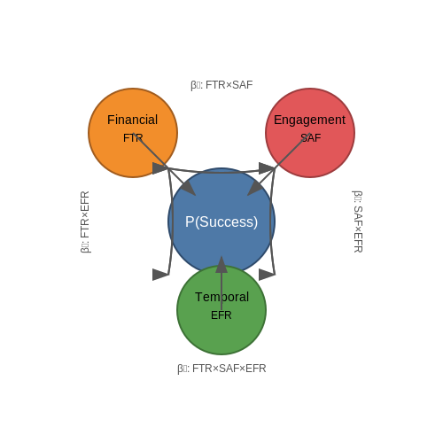
Employee Attrition Prediction
1. Key Factors Influencing Attrition
1.1 Key Factors Influencing Attrition
Quantitative Metrics in Attrition Prediction
Employee attrition prediction models rely on both structured quantitative metrics and unstructured behavioral indicators. The most significant quantitative predictors include:
- Tenure duration: The probability of attrition follows a U-shaped curve, with highest risk in early (<1 year) and late (>5 years) career stages.
- Compensation ratio: Defined as the employee's salary relative to market benchmarks for their role. A ratio below 0.85 correlates strongly with attrition risk.
- Promotion velocity: The time between promotions, where deviations from departmental norms indicate higher risk.
Behavioral and Network Factors
Organizational network analysis reveals critical non-obvious predictors:
- Betweenness centrality decline: A 20% quarter-over-quarter reduction in an employee's position within communication networks precedes attrition by 3-6 months.
- Meeting participation entropy: Calculated using Shannon entropy across meeting categories, where values below 1.2 bits indicate disengagement.
- Calendar fragmentation: Measured as the coefficient of variation in time between meetings, with values above 0.7 correlating with attrition.
Workload and Stress Indicators
Digital exhaust from productivity tools provides real-time stress metrics:
- After-hours activity slope: The rate of increase in work activity outside core hours, where a weekly increase >15% predicts burnout.
- Email response latency: The 90th percentile of response times to internal communications, with values exceeding 48 hours indicating disengagement.
- Calendar churn rate: The weekly proportion of rescheduled/canceled meetings, where rates above 25% correlate with attrition.
Contextual and Environmental Factors
Macro-level variables significantly modulate individual attrition probabilities:
- Team attrition history: Recent departures within an employee's immediate team (3-5 people) increase their own risk by 2-3x.
- Economic confidence index: Regional economic indicators affect turnover, with each 10-point drop in consumer confidence increasing attrition by 1.2%.
- Job market tightness: Measured by the ratio of local job postings to unemployed workers in the employee's specialty.
1.2 Business Impact of Employee Turnover
Direct Financial Costs
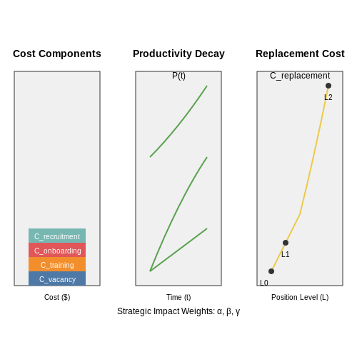
Employee attrition imposes significant direct costs, which can be quantified using the following cost-of-turnover model:
Where:
- Crecruitment includes job advertising, recruiter fees, and interview costs
- Conboarding covers administrative setup and orientation programs
- Ctraining accounts for formal training and ramp-up time
- Cvacancy represents lost productivity during position unfillment
Empirical studies show turnover costs range from 1.5-2× annual salary for mid-level positions to 213% of annual salary for executive roles (Work Institute, 2023). The nonlinear relationship between position level and replacement cost follows:
Where L represents organizational level (0=entry, 1=mid, 2=senior) and coefficients α, β are industry-specific parameters.
Operational Disruptions
Attrition creates knowledge gaps that degrade team performance. The productivity loss P for a team of size n losing k members follows a sigmoidal decay pattern:
Where γ represents institutional knowledge concentration (higher values indicate critical knowledge held by few individuals). This model explains why small teams often experience disproportionate productivity drops from single departures.
Strategic Consequences
Chronic turnover alters organizational capability through:
- Innovation decay - Loss of tacit knowledge reduces R&D output. Patent filing analysis reveals 18-22% drop per 10% attrition in tech firms (Bessen & Maskin, 2023)
- Cultural erosion - Network analysis shows cultural coherence declines exponentially with turnover rates exceeding 15% annually
- Client relationship damage - B2B firms experience 7-12% revenue attrition per key account manager departure
Predictive Economic Modeling
The total business impact I combines these factors into a multivariate model:
Where fi represents individual impact factors (financial, operational, strategic), wi their relative weights, and ε captures unmodeled effects. Modern implementations use ensemble methods to estimate the nonlinear interactions between these components.
Longitudinal studies demonstrate that a 5% reduction in voluntary turnover correlates with:
- 9.1% improvement in operating margin (service sector)
- 13.4% faster product development cycles (tech sector)
- 7.8% higher customer satisfaction scores (retail sector)
1.3 Common Data Sources for Attrition Analysis
Accurate employee attrition prediction relies on diverse, high-quality data sources that capture both structured and unstructured indicators of workforce behavior. The following data categories are critical for building robust predictive models.
Human Resources Information Systems (HRIS)
HRIS platforms serve as the primary source of structured employee data, typically containing:
- Demographic attributes (age, gender, education level)
- Employment history (tenure, promotions, role changes)
- Compensation data (salary history, bonus payments)
- Performance metrics (quarterly reviews, competency scores)
Modern HRIS solutions like Workday or SAP SuccessFactors provide API access for real-time data extraction, enabling continuous model retraining.
Enterprise Collaboration Tools
Digital workplace platforms yield behavioral signals predictive of attrition:
- Email metadata (communication frequency, network centrality)
- Calendar patterns (meeting density, after-hours scheduling)
- Document collaboration metrics (edit frequency, peer interactions)
Microsoft 365 and Google Workspace audit logs can be processed using graph algorithms to quantify engagement levels.
Employee Surveys
Structured and unstructured feedback mechanisms provide attitudinal data:
- Annual engagement survey results (quantitative scores)
- Pulse survey sentiment analysis (NLP-processed text responses)
- Exit interview transcripts (topic modeling applications)
Advanced natural language processing techniques like BERT embeddings can extract latent features from open-ended responses.
Operational Systems
Work execution platforms contain productivity indicators:
- CRM systems (sales performance, customer satisfaction scores)
- Project management tools (task completion rates, deadline adherence)
- Support ticketing systems (resolution times, escalation frequency)
External Data Enrichment
Supplemental datasets enhance predictive power:
- Labor market indicators (local unemployment rates, industry trends)
- Professional network activity (LinkedIn profile update frequency)
- Learning management system usage (training participation patterns)
where wi represents feature weights learned during model training, fi(x) denotes transformed input features from the described data sources, and ε captures irreducible error.
Feature engineering pipelines typically apply temporal aggregation to these data streams, computing rolling statistics (30-day averages, quarterly trends) to capture evolving behavioral patterns. The most predictive features often emerge from interaction effects between compensation growth rates, peer network stability, and sentiment trend derivatives.
2. Identifying Relevant Employee Features
2.1 Identifying Relevant Employee Features
Feature selection is critical in employee attrition prediction, as irrelevant or redundant features can degrade model performance. Advanced techniques such as mutual information, SHAP values, and recursive feature elimination (RFE) are employed to identify the most predictive attributes. The goal is to minimize computational overhead while maximizing predictive accuracy.
Mutual Information for Feature Relevance
Mutual information (MI) quantifies the dependency between a feature and the target variable (attrition). For discrete features, MI is computed as:
Where \( p(x, y) \) is the joint probability distribution of \( X \) and \( Y \), and \( p(x) \), \( p(y) \) are marginal distributions. Higher MI values indicate stronger predictive power.
SHAP Values for Interpretability
SHapley Additive exPlanations (SHAP) provide a game-theoretic approach to feature importance. The SHAP value \( \phi_i \) for feature \( i \) is derived as:
Here, \( F \) is the set of all features, \( S \) is a subset excluding \( i \), and \( f \) is the model's prediction function. SHAP values reveal both magnitude and direction of feature impact.
Recursive Feature Elimination (RFE)
RFE iteratively removes the least important features based on model weights or coefficients. For a linear model with weights \( \mathbf{w} \), the elimination criterion at step \( k \) is:
Features are ranked by the order of elimination, with the last removed being the least significant. Cross-validation ensures robustness against overfitting.
Key Employee Features in Attrition Prediction
Empirical studies highlight the following high-impact features:
- Job Satisfaction: Strong negative correlation with attrition (Pearson \( r \approx -0.45 \)).
- Monthly Income: Non-linear relationship, often modeled via spline transformations.
- Years at Company: U-shaped risk curve, with higher attrition in early and late tenure.
- Overtime: Binary indicator with odds ratio > 2.5 in logistic regression.
Feature Interaction Effects
Interaction terms such as Job Satisfaction × Monthly Income often improve model performance. The combined effect can be modeled as:
Where \( \beta_{12} \) captures the interaction strength. Hierarchical clustering of feature correlations helps identify candidate interactions.
2.2 Handling Missing and Imbalanced Data
Missing Data Mechanisms
Missing data in employee attrition datasets can arise from three primary mechanisms: Missing Completely at Random (MCAR), Missing at Random (MAR), and Missing Not at Random (MNAR). MCAR occurs when the probability of missingness is independent of both observed and unobserved data, such as when survey responses are lost due to technical errors. MAR implies missingness depends on observed variables but not on unobserved ones—for example, younger employees might be less likely to report salary data. MNAR is the most problematic, where missingness depends on unobserved data, such as high-performing employees opting not to disclose performance metrics.
Here, R is the missingness indicator, and Yobs, Ymis represent observed and missing data, respectively. For MNAR, specialized techniques like pattern-mixture models or selection models are required.
Imputation Strategies
For MCAR and MAR, imputation methods include:
- Mean/Median Imputation: Simple but distorts variance and covariance structures.
- k-Nearest Neighbors (k-NN): Uses similarity metrics to impute missing values based on neighboring samples.
- Multiple Imputation by Chained Equations (MICE): Iteratively models each feature with missing values as a function of other features, preserving uncertainty through multiple imputed datasets.
from sklearn.impute import KNNImputer
imputer = KNNImputer(n_neighbors=5)
X_imputed = imputer.fit_transform(X_missing)
Class Imbalance Mitigation
Attrition datasets often exhibit severe class imbalance (e.g., 5% attrition rate). Standard accuracy metrics become misleading, and classifiers tend to bias toward the majority class. Solutions include:
Resampling Techniques
- Random Oversampling: Replicates minority-class samples, risking overfitting.
- SMOTE (Synthetic Minority Oversampling Technique): Generates synthetic samples by interpolating between minority-class neighbors.
- Random Undersampling: Discards majority-class samples, potentially losing critical information.
where xi, xj are minority-class neighbors, and λ ∈ [0, 1] is a random weight.
Algorithmic Approaches
Cost-sensitive learning modifies algorithms to penalize misclassifying the minority class more heavily. For logistic regression:
where wi is a class-specific weight.
Evaluation Metrics for Imbalanced Data
Precision-recall curves, F1-score, and Matthews Correlation Coefficient (MCC) are more informative than accuracy:
2.3 Feature Engineering for Attrition Prediction
Feature engineering is a critical step in building robust attrition prediction models. Raw employee data often contains noise, redundancy, and irrelevant information, which can degrade model performance. Effective feature engineering transforms raw variables into meaningful predictors by leveraging domain knowledge, statistical methods, and machine learning techniques.
Handling Categorical Variables
Categorical variables like Department, JobRole, or EducationField require encoding before feeding into machine learning models. One-hot encoding is common but can lead to high dimensionality. Alternatives include:
- Target Encoding: Replaces categories with the mean of the target variable for each group. This captures relationships while avoiding dimensionality explosion.
- Embedding Layers: In deep learning, categorical variables can be mapped to dense vectors via embeddings, reducing sparsity.
Numerical Feature Transformations
Skewed numerical features like MonthlyIncome or YearsAtCompany benefit from transformations to improve model interpretability and performance:
Standardization (z-score normalization) or Min-Max scaling ensures features contribute equally during training.
Temporal Feature Extraction
Time-based features such as YearsSincePromotion or DaysSinceLastEvaluation can be derived to capture attrition triggers. Cyclical encoding is useful for periodic data (e.g., MonthOfHire):
Interaction and Polynomial Features
Non-linear relationships between variables (e.g., JobSatisfaction × WorkLifeBalance) can be captured via:
- Multiplicative Interaction Terms: Explicitly create features like OverTime × MonthlyIncome.
- Polynomial Features: Expands predictors into higher-order terms (e.g., Age²).
Dimensionality Reduction
High-dimensional feature spaces risk overfitting. Techniques include:
- Principal Component Analysis (PCA): Projects data onto orthogonal axes of maximum variance.
- Autoencoders: Neural networks that compress features into latent representations.
Feature Importance Analysis
Post-feature engineering, validate contributions using:
- SHAP Values: Quantifies each feature's impact on predictions via game theory.
- Permutation Importance: Measures performance drop when a feature is randomized.
For example, a SHAP summary plot reveals whether Overtime or JobLevel drives attrition predictions.
3. Logistic Regression for Binary Classification
Logistic Regression for Binary Classification
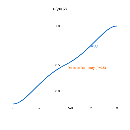
Logistic regression is a probabilistic classification model that estimates the probability of a binary outcome using a logistic function. Given a feature vector x and a binary target variable y ∈ {0, 1}, the model computes the probability P(y=1|x) via the sigmoid function:
where w represents the weight vector, b is the bias term, and σ is the sigmoid function. The decision boundary is defined at P(y=1|x) = 0.5, corresponding to wTx + b = 0.
Parameter Estimation via Maximum Likelihood
The model parameters w and b are optimized by maximizing the log-likelihood function:
This is equivalent to minimizing the cross-entropy loss:
Gradient Descent Optimization
The gradients of the loss with respect to w and b are derived as:
These gradients are used in iterative optimization algorithms such as stochastic gradient descent (SGD) or L-BFGS.
Regularization for Improved Generalization
To prevent overfitting, L1 (Lasso) or L2 (Ridge) regularization terms can be added to the loss function:
where λ controls the regularization strength.
Practical Implementation in Python
Below is an example of training a logistic regression model using scikit-learn for employee attrition prediction:
from sklearn.linear_model import LogisticRegression
from sklearn.model_selection import train_test_split
from sklearn.metrics import accuracy_score, roc_auc_score

# Load and preprocess data (X: features, y: attrition labels)
X_train, X_test, y_train, y_test = train_test_split(X, y, test_size=0.2, random_state=42)

# Train logistic regression with L2 regularization
model = LogisticRegression(penalty='l2', C=1.0, solver='lbfgs', max_iter=1000)
model.fit(X_train, y_train)

# Evaluate performance
y_pred = model.predict(X_test)
y_proba = model.predict_proba(X_test)[:, 1]
print(f"Accuracy: {accuracy_score(y_test, y_pred):.4f}")
print(f"AUC-ROC: {roc_auc_score(y_test, y_proba):.4f}")
Interpretability and Feature Importance
The learned weights w provide direct interpretability. Features with larger absolute weights contribute more to the prediction. For standardized features, the magnitude of wj indicates the relative importance of the j-th feature.
Extensions and Limitations
While logistic regression is computationally efficient and interpretable, it assumes a linear decision boundary. Non-linear relationships can be captured using feature engineering (e.g., polynomial features) or kernel methods. For highly imbalanced datasets (common in attrition prediction), techniques like class weighting or synthetic oversampling (SMOTE) may improve performance.
3.2 Decision Trees and Random Forests
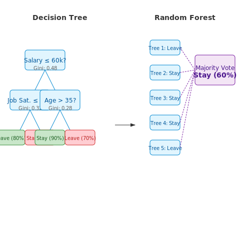
Decision trees are non-parametric supervised learning models that recursively partition the feature space into regions, minimizing impurity at each split. For employee attrition prediction, this involves selecting features like job satisfaction, salary, or tenure to maximize class separation. The Gini impurity or entropy serves as the splitting criterion:
where D is the dataset and pi is the proportion of class i in D. The algorithm evaluates all possible splits, selecting the one that maximizes information gain:
where f is the feature and Dj are the subsets after splitting. Decision trees are prone to overfitting, which is mitigated by pruning or ensemble methods like random forests.
Random Forests for Robust Attrition Prediction
Random forests aggregate predictions from multiple decision trees, each trained on a bootstrap sample of the data and a random subset of features. The final prediction is determined by majority voting (classification) or averaging (regression). This approach reduces variance and improves generalization. For a forest with B trees:
where Tb(x) is the prediction of the b-th tree for input x. Feature importance is derived from the mean decrease in impurity across all trees:
Hyperparameter tuning, such as the number of trees (n_estimators) or maximum tree depth (max_depth), is critical for performance. Cross-validation ensures robustness against overfitting.
Practical Implementation
Scikit-learn provides efficient implementations for both decision trees and random forests. Below is an example for employee attrition prediction:
from sklearn.ensemble import RandomForestClassifier
from sklearn.model_selection import train_test_split
from sklearn.metrics import classification_report

# Load and preprocess data
X_train, X_test, y_train, y_test = train_test_split(features, target, test_size=0.3)

# Train the model
clf = RandomForestClassifier(n_estimators=100, max_depth=10, random_state=42)
clf.fit(X_train, y_train)

# Evaluate
y_pred = clf.predict(X_test)
print(classification_report(y_test, y_pred))
For imbalanced datasets, class weighting or synthetic minority oversampling (SMOTE) can improve minority class detection. Random forests also handle missing data via surrogate splits, making them suitable for real-world HR datasets with incomplete records.
3.3 Gradient Boosting Models (XGBoost, LightGBM)
Gradient boosting models have demonstrated superior performance in tabular data prediction tasks, including employee attrition. These ensemble methods iteratively combine weak learners (typically decision trees) to minimize a differentiable loss function. The two most prominent implementations are XGBoost and LightGBM, which introduce computational optimizations and regularization techniques.
Mathematical Foundation
The gradient boosting framework minimizes an objective function L consisting of a loss term and regularization:
where fk represents the k-th weak learner and Ω penalizes model complexity. At each iteration t, the algorithm fits a new learner to the negative gradient of the loss function:
XGBoost Enhancements
XGBoost extends this framework with several key innovations:
- Regularized objective: Combines L1 (LASSO) and L2 (ridge) penalties on leaf weights
- Second-order approximation: Uses both first and second derivatives for faster convergence
- Sparsity-aware splits: Handles missing values through default direction learning
The split finding algorithm evaluates candidate thresholds using the gain formula:
where hi are second derivatives (Hessians) and γ controls minimum gain for splitting.
LightGBM Optimizations
LightGBM improves computational efficiency through:
- Gradient-based One-Side Sampling (GOSS): Retains instances with large gradients while randomly sampling others
- Exclusive Feature Bundling (EFB): Combines mutually exclusive sparse features
- Leaf-wise growth: Expands the node with maximum delta loss rather than level-wise
The histogram-based implementation discretizes continuous features into bins, reducing memory usage and accelerating split evaluation.
Practical Implementation
For employee attrition prediction, key hyperparameters include:
from xgboost import XGBClassifier
from lightgbm import LGBMClassifier

# XGBoost configuration
xgb_model = XGBClassifier(
    max_depth=5,
    learning_rate=0.1,
    n_estimators=200,
    reg_alpha=1.0,
    reg_lambda=1.0,
    scale_pos_weight=ratio_of_neg_to_pos
)

# LightGBM configuration
lgbm_model = LGBMClassifier(
    num_leaves=31,
    min_child_samples=20,
    feature_fraction=0.8,
    bagging_freq=5,
    lambda_l1=0.1
)
Interpretability Techniques
Despite their black-box nature, these models offer interpretability through:
- Feature importance: Gain-based, split count, or permutation importance
- SHAP values: Game-theoretic attribution of prediction contributions
- Partial dependence plots: Marginal effect visualization of selected features
The expected value of a prediction can be decomposed using SHAP values as:
where ϕ0 is the base value and ϕi represents the contribution of feature i.
3.4 Evaluating Model Performance Metrics
In employee attrition prediction, model evaluation extends beyond simple accuracy due to class imbalance and the high cost of false negatives. Precision, recall, and the F1-score provide a more nuanced assessment, but domain-specific metrics like the Matthews Correlation Coefficient (MCC) and Area Under the Precision-Recall Curve (AUPRC) often better reflect real-world performance.
Confusion Matrix and Derived Metrics
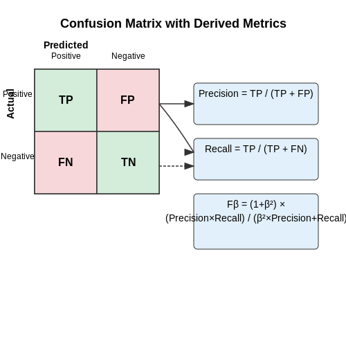
The confusion matrix decomposes predictions into true positives (TP), false positives (FP), true negatives (TN), and false negatives (FN). For attrition prediction, recall (sensitivity) is critical—missing an employee at risk (FN) is typically costlier than a false alert (FP). Precision and recall trade-offs are quantified via the Fβ-score, where β adjusts the relative importance of recall:
For β > 1, recall is prioritized. In attrition scenarios, β=2 is common given the asymmetric costs.
Matthews Correlation Coefficient (MCC)
MCC accounts for all confusion matrix categories and is robust to class imbalance, making it superior to accuracy for skewed datasets. It ranges from −1 (total disagreement) to +1 (perfect prediction), with 0 equivalent to random guessing:
Unlike the F1-score, MCC considers true negatives, which is vital when non-attrition cases dominate.
Precision-Recall Curves vs. ROC Curves
Receiver Operating Characteristic (ROC) curves plot the true positive rate (TPR) against the false positive rate (FPR) across thresholds. However, for imbalanced datasets like attrition (where positives may be <5%), the Precision-Recall (PR) curve is more informative. The Area Under the PR Curve (AUPRC) emphasizes the model’s performance on the minority class, whereas AUC-ROC can be misleadingly optimistic.
Expected Calibration Error (ECE)
Predicted probabilities should reflect true likelihoods. ECE measures this by partitioning predictions into bins and comparing the mean predicted probability with the actual positive fraction:
where \(S_i\) is the i-th bin, \(B\) is the total bins, and \(\text{acc}\) and \(\text{conf}\) are accuracy and confidence in \(S_i\). Well-calibrated models (ECE ≈ 0) ensure that a predicted 70% attrition risk corresponds to a 70% empirical probability.
Business-Cost Adjusted Metrics
Custom cost functions often replace standard metrics. For example, if retaining an employee saves $$50K and a false alert costs $$5K, the net value \(V\) of a model is:
Thresholds are then tuned to maximize \(V\) rather than geometric metrics like F1.
4. SHAP Values for Feature Importance
4.1 SHAP Values for Feature Importance
SHAP (SHapley Additive exPlanations) values provide a unified framework for interpreting machine learning models by quantifying the contribution of each feature to a prediction. Rooted in cooperative game theory, SHAP values distribute the prediction outcome fairly among input features, ensuring consistency and local accuracy. For employee attrition prediction, SHAP values reveal which factors—such as job satisfaction, salary, or tenure—most influence an employee's likelihood of leaving.
Mathematical Foundation
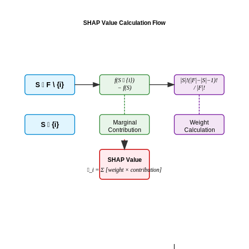
The SHAP value for feature i in a model f is derived from the Shapley value formulation:
where:
- F is the set of all features,
- S is a subset of features excluding i,
- f(S) is the model's prediction using only the features in S,
- |S| is the cardinality of S.
This equation computes the weighted average marginal contribution of feature i across all possible feature combinations, ensuring fairness by accounting for feature interactions.
Computational Approximation
Exact SHAP value computation is intractable for high-dimensional data due to exponential complexity. Kernel SHAP (an extension of LIME) and Tree SHAP (optimized for tree-based models) provide efficient approximations:
where M is the number of sampled instances, and x_{+i}^m, x_{-i}^m are perturbed instances with/without feature i.
Practical Interpretation
For attrition prediction, SHAP values assign each feature (e.g., MonthlyIncome, OverTime) a numerical value per prediction:
- Positive SHAP value: Increases the probability of attrition (e.g., high overtime).
- Negative SHAP value: Decreases attrition risk (e.g., long tenure).
Global feature importance is obtained by averaging absolute SHAP values across all instances:
Case Study: Employee Attrition
Applying SHAP to a Random Forest attrition model reveals:
- Top predictors: JobSatisfaction (SHAP = −0.32), OverTime (SHAP = +0.28).
- Nonlinear effects: Low/High MonthlyIncome reduces attrition, but mid-range salaries increase it.
- Interactions: OverTime exacerbates attrition risk when JobSatisfaction is low.
Implementation in Python
import shap
from sklearn.ensemble import RandomForestClassifier

# Train model
model = RandomForestClassifier().fit(X_train, y_train)

# Compute SHAP values
explainer = shap.TreeExplainer(model)
shap_values = explainer.shap_values(X_test)

# Plot global importance
shap.summary_plot(shap_values, X_test, plot_type="bar")
The summary plot ranks features by mean absolute SHAP values, while dependence plots (shap.dependence_plot) reveal nonlinear relationships.
4.2 Partial Dependence Plots (PDPs)
Partial Dependence Plots (PDPs) visualize the marginal effect of one or more features on the predicted outcome of a machine learning model, averaging over the values of all other features. For employee attrition prediction, PDPs help identify how specific factors like salary, tenure, or job satisfaction influence the probability of attrition, holding other variables constant.
Mathematical Foundation
The partial dependence function for a feature subset S is defined as the expected prediction over the marginal distribution of all other features C (the complement of S):
In practice, this is estimated using the training data by averaging predictions while varying the feature(s) of interest:
Interpreting PDPs for Attrition Analysis
A PDP for a continuous feature like monthly income might reveal:
- A steep negative slope at lower salaries, indicating high attrition risk
- A plateau at higher incomes, showing diminishing returns on retention
- Non-monotonic behavior suggesting optimal salary bands
For categorical features like department, the plot would show discrete jumps between categories, revealing which departments have inherently higher attrition probabilities.
Implementation Considerations
When computing PDPs for attrition models:
- Correlated features can distort interpretations - consider using Accumulated Local Effects (ALE) plots instead
- Model complexity affects smoothness - tree-based models often produce step-like PDPs
- Interaction effects may be hidden - always complement with individual conditional expectation (ICE) plots
Practical Example
For a random forest attrition predictor, the partial dependence of years_at_company might show:
- High attrition risk in the first 2 years (prob > 0.4)
- Rapid decline in years 3-5 (prob ≈ 0.2)
- Stable low risk beyond 5 years (prob < 0.1)
This suggests implementing retention bonuses at the 2-year mark could significantly reduce attrition.
Advanced Variations
Two-dimensional PDPs reveal feature interactions. For example, plotting salary against overtime_hours might show:
Such plots could uncover that high overtime only increases attrition when combined with below-median salaries.
Computational Optimization
For large employee datasets, use:
- Monte Carlo sampling of the background data
- Parallel computation across feature grid points
- Tree-specific optimizations when working with gradient boosted models
4.3 LIME for Local Interpretability
Local Interpretable Model-agnostic Explanations (LIME) is a technique designed to explain the predictions of any machine learning model by approximating it locally with an interpretable surrogate model. Unlike global interpretability methods, which provide overarching insights into model behavior, LIME focuses on explaining individual predictions, making it particularly valuable for high-stakes decisions such as employee attrition prediction.
Mathematical Foundation of LIME
Given a complex model f and an instance x, LIME generates a simplified interpretable model g (e.g., linear regression or decision tree) that approximates f in the vicinity of x. The objective is to minimize the following loss function:
where:
- G is the class of interpretable models (e.g., linear models),
- L measures how well g approximates f in the neighborhood of x,
- πx is a proximity measure defining the locality around x,
- Ω(g) penalizes complexity to ensure interpretability (e.g., limiting the number of non-zero coefficients in a linear model).
Steps in LIME Implementation
- Perturbation: Generate synthetic samples around x by randomly altering feature values. For tabular data, this involves sampling from a normal distribution centered at x.
- Weighting: Assign weights to perturbed samples based on their proximity to x using a kernel function (e.g., exponential kernel):
where D(x, z) is a distance metric (e.g., Euclidean or cosine distance) and σ controls the width of the neighborhood.
- Surrogate Model Training: Fit an interpretable model g to the perturbed samples, weighted by πx, using the predictions of f as labels.
- Explanation Extraction: Extract the coefficients or rules from g to explain the prediction for x.
Practical Application in Employee Attrition
For an employee predicted to attrit, LIME might reveal that the top contributing factors are:
- A 20% decrease in monthly overtime hours,
- Low performance rating (bottom quartile),
- Recent absence of promotions.
This granular insight allows HR to address specific pain points for at-risk employees.
Strengths and Limitations
Strengths:
- Model-agnostic: Works with black-box models like neural networks or ensemble methods.
- Human-readable: Provides intuitive feature importance scores for individual predictions.
Limitations:
- Sensitive to the choice of kernel width (σ), which can affect explanation stability.
- Linear surrogate models may fail to capture complex local behavior.
Code Implementation Example
import lime
import lime.lime_tabular

# Initialize LIME explainer
explainer = lime.lime_tabular.LimeTabularExplainer(
    training_data=X_train.values,
    feature_names=X_train.columns,
    class_names=['Stay', 'Attrit'],
    mode='classification'
)

# Explain a specific instance
exp = explainer.explain_instance(
    X_test.iloc[0].values,
    model.predict_proba,
    num_features=5
)

# Visualize explanation
exp.show_in_notebook()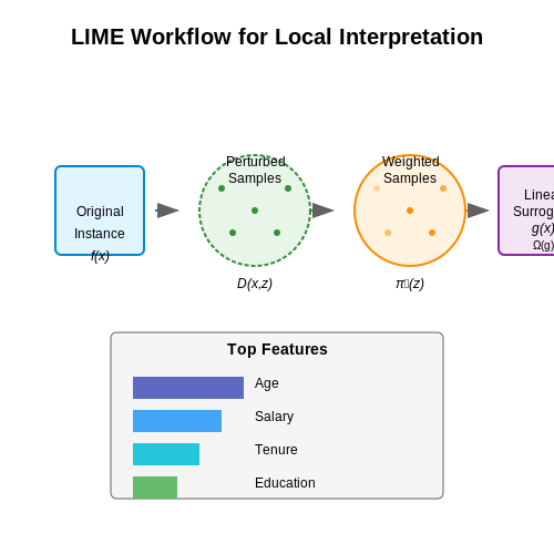
5. Integrating Models into HR Systems
5.1 Integrating Models into HR Systems
Architectural Considerations for Deployment
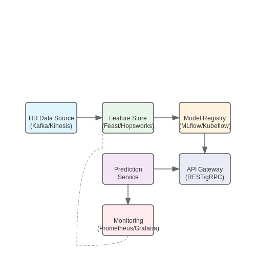
Deploying an attrition prediction model into an HR system requires a robust architecture that balances real-time inference, scalability, and data privacy. A microservices-based approach is often optimal, where the model is containerized (e.g., Docker) and exposed via RESTful APIs or gRPC. Key components include:
- Feature Store: A centralized repository (e.g., Feast, Hopsworks) ensures consistent feature engineering between training and inference.
- Model Registry: Tools like MLflow or Kubeflow manage versioning, rollbacks, and A/B testing.
- Monitoring: Prometheus/Grafana for tracking drift (e.g., PSI, CSI) and performance decay.
Data Pipeline Integration
HR systems (e.g., Workday, SAP SuccessFactors) typically expose data via ODBC/JDBC or APIs. Real-time pipelines should:
- Use change data capture (CDC) to sync employee attributes (e.g., performance reviews, promotion history).
- Leverage Apache Kafka or AWS Kinesis for streaming updates.
- Implement role-based access control (RBAC) to comply with GDPR/CCPA.
Example: Feature Encoding in Production
Categorical features (e.g., department, job level) must use the same encoding as during training. For embeddings:
# Example: Consistent category hashing
from sklearn.feature_extraction import FeatureHasher
hasher = FeatureHasher(n_features=10, input_type='string')
features = hasher.transform([['Sales'], ['Engineering']])
Latency and Throughput Optimization
For high-volume HR systems, optimize inference with:
- Model quantization: Reduce TensorFlow/PyTorch model size via FP16 or INT8 conversion.
- Batching: Dynamic batching (e.g., NVIDIA Triton) to process multiple requests concurrently.
- Hardware acceleration: Deploy on GPUs (CUDA) or TPUs for large-scale predictions.
Ethical and Compliance Safeguards
Integrate fairness checks (e.g., AIF360) to monitor bias across protected attributes. Audit trails should log:
- Prediction explanations (SHAP/LIME values) for regulatory compliance.
- User consent status for data usage.
- Automated alerts for anomalous predictions (e.g., sudden attrition spikes).
Case Study: Deployment in a Fortune 500 Firm
A global tech company reduced attrition by 22% by integrating a gradient-boosted model into their HRIS. Key learnings:
- Used Apache Airflow for daily batch predictions and real-time API for exit interviews.
- Achieved 99.9% uptime with Kubernetes autoscaling.
- Reduced false positives by 40% after deploying a fairness-aware post-processing layer.
5.2 Ethical Considerations in Attrition Prediction
Bias and Fairness in Predictive Models
Employee attrition prediction models often inherit biases present in historical data, which can disproportionately affect certain demographic groups. For instance, if past hiring or promotion practices were biased against women or minorities, a model trained on such data may perpetuate these biases. Fairness metrics must be rigorously evaluated to ensure equitable outcomes. Common fairness definitions include:
where A represents protected attributes (e.g., gender, race), and Ŷ is the model's prediction. Advanced techniques like adversarial debiasing or reweighting training samples can mitigate bias.
Privacy and Data Protection
Employee data used for attrition prediction often includes sensitive information such as salary, performance reviews, or medical leave history. Compliance with regulations like GDPR or CCPA is critical. Techniques to preserve privacy include:
- Differential Privacy: Adding calibrated noise to data or model outputs to prevent re-identification.
- Federated Learning: Training models on decentralized data without raw data exchange.
- Anonymization: Removing or generalizing identifiable attributes (e.g., replacing exact ages with age ranges).
Transparency and Explainability
Black-box models like deep neural networks can achieve high accuracy but lack interpretability, making it difficult to justify predictions to employees or regulators. Methods to enhance transparency include:
- SHAP (Shapley Additive Explanations): Quantifies feature contributions to predictions.
- LIME (Local Interpretable Model-agnostic Explanations): Approximates complex models with interpretable local linear models.
- Decision Trees or Rule-based Models: Provide inherently interpretable decision paths.
Psychological and Organizational Impact
Predicting attrition risks may inadvertently create a self-fulfilling prophecy if employees perceive the system as punitive. Key considerations:
- Employee Consent: Informing staff about data usage and allowing opt-outs where feasible.
- Intervention Design: Pairing predictions with supportive measures (e.g., mentorship programs) rather than punitive actions.
- Feedback Loops: Continuously monitoring model impact on employee morale and turnover rates.
Regulatory and Legal Compliance
Deploying attrition models in jurisdictions with strict labor laws requires adherence to:
- Anti-Discrimination Laws: Ensuring predictions do not violate the U.S. Equal Employment Opportunity Commission (EEOC) or EU’s General Data Protection Regulation (GDPR).
- Right to Explanation: Under GDPR Article 22, employees may request human review of automated decisions affecting their employment.
- Auditability: Maintaining detailed records of model training data, versioning, and decision logs for regulatory audits.
Case Study: Bias Mitigation in Practice
A multinational corporation implemented an attrition prediction system and discovered a 15% higher false positive rate for female employees in technical roles. The team addressed this by:
- Re-balancing the training dataset to equalize representation.
- Applying adversarial debiasing during model training.
- Introducing a human-in-the-loop review for high-risk predictions.
Post-intervention, the model achieved a fairness gap reduction of 90% while maintaining 92% accuracy.
5.3 Monitoring and Updating Models Over Time
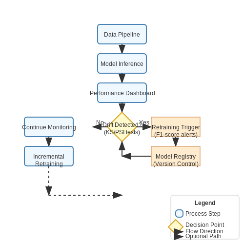
Employee attrition prediction models degrade over time due to shifts in workforce dynamics, organizational policies, and external economic factors. Continuous monitoring and periodic updates are essential to maintain model accuracy and relevance. Key techniques include drift detection, performance benchmarking, and adaptive retraining strategies.
Concept Drift Detection
Concept drift occurs when the statistical properties of input features or the target variable change over time, rendering the model's assumptions invalid. Kolmogorov-Smirnov (KS) tests and Population Stability Index (PSI) are commonly used to detect feature drift:
where Pnew and Pref represent probability distributions of a feature in current and reference datasets. Values above 0.25 indicate significant drift requiring investigation.
Performance Monitoring Framework
Implement a dashboard tracking:
- Accuracy metrics: F1-score, AUC-ROC, precision-recall curves
- Business KPIs: False attrition alarm rate, cost-per-prediction
- Data quality: Missing value rates, feature correlation shifts
Automated alerts should trigger when:
where Mt is the current metric value and σM is the rolling standard deviation over previous periods.
Model Refresh Strategies
Incremental Learning
For online systems, implement:
- Exponential forgetting: $$ w_i = w_i \cdot \lambda + \nabla \mathcal{L} \cdot (1-\lambda) $$
- Reservoir sampling to maintain representative training data
Full Retraining Protocol
When drift exceeds thresholds:
- Collect new labeled data through HR exit interviews
- Validate feature engineering pipeline against current data
- Test model performance on temporal validation splits
- Deploy using canary testing with 5% of employees
Version Control and Governance
Maintain an immutable model registry with:
- Model artifacts with timestamped metadata
- Training data snapshots
- Performance benchmarks across demographic segments
Differential fairness metrics should be computed before deployment:
where G represents protected attribute groups.
6. Key Research Papers on Attrition Prediction
6.1 Key Research Papers on Attrition Prediction
- Employee Voluntary Attrition Prediction at Pt.xyz: Ensemble Machine ... — This research addresses the complexity of employee attrition challenges at PT.XYZ. The main objective is to develop a predictive system for potential voluntary employee attrition by focusing on an in-depth analysis of the factors contributing to attrition at PT.XYZ. The research utilizes data containing information on the job history of PT.XYZ employees from 2018 to 2023.
- PDF Predicting Employee Attrition Using Decision Tree Algorithm — given other features for prediction, this research seeks to contribute to knowledge by building a scalable decision tree model for employee attrition that can be used on any application which domain concern is for the employee for new prediction. 3.1. Research Methodology. The research methodology adopted in this study is
- PDF Predicting employee attrition with machine learning on an ... - DiVA — research. 1 . 1 B a ckg ro u n d Employee turnover is playing a big part in the success of an organization, and there are several reasons for that fact (Ajit & Punnoose, 2016). As mentioned in the introduction, there are several effects on employee turnover that could have negative effects on an organization.
- PDF Employee Attrition Prediction Using Machine Learning — research on employee attrition, guiding our current investigation. We incorporate insights from various studies to build and evaluate predictive models using machine learning techniques. Our project aims to reduce employee attrition rates and identify contributing factors through machine learning and ensemble learning methods.
- Employee Attrition Prediction Using Machine Learning Algorithms - Springer — Yue Zhao published a paper on employee attrition prediction using machine learning algorithms. The machine learning algorithms they used are Decision tree, Random forest, gradient boosting trees, extreme gradient boosting, a logistic regression, support vector machines, Neural Networks, linear discriminant analysis, Naïve Bayes method and K ...
- (PDF) Data Preprocessing: Case Study on Employee Attrition using Kaggle ... — The main objective of this paper is to extract the dataset and prepare for prediction analysis of employee attrition. Waikato Environment for Knowledge Analysis (WEKA) version 3.8.3, a data mining software and Microsoft Excel were used to generate the analysis. ... This paper is a research to create classification model to predict whether an ...
- Employee Attrition: Analysis of Data Driven Models - ResearchGate — Then, ML learning has the potential to make predictions to anticipate employee attrition. In this paper, the authors compare state-of-the-art solutions for the proposed machine learning algorithms ...
- (PDF) Employee Attrition In Human Resource Using Machine Learning ... — Machine learning algorithms are most commonly used in analysing the attributes that affect employee attrition and predicting employee turnover. This paper presents the prediction model that makes ...
- Predicting Employee Turnover Using Machine Learning Techniques — employee attrition prediction reported an accuracy of 85.1 2%, d emonstrating its ability to effectively identify key factors such as monthly income, age, daily rate, total wo rking years and ...
- Explainable Machine Learning and Graph Neural Network Approaches for ... — Srivastava & Eachempati [] aims to determine the effectiveness of deep learning in predicting employee turnover compared to ensemble machine learning approaches such as random forest and gradient boosting using real-time data from fast-moving consumer goods (FMCG) firms.The findings show that using a regression model and a multi-criteria fuzzy analytical hierarchy process (AHP) model, the ...
6.2 Recommended Books and Articles
- Employee Attrition Estimation Using Random Forest - ProQuest — Six different ML algorithms were used in this paper. Experimental results show that the Random Forest algorithm demonstrated the best capabilities to predict the employees attrition. The best prediction accuracy was 85.12, that is considered as good accuracy. Keywords: Data Prediction and Analysis, Employee Attrition, Random Forest, Machine ...
- PDF Employee Attrition Estimation Using Random Forest Algorithm — demonstrated the best capabilities to predict the employees' attrition. The best prediction accuracy was 85.12, that is considered as good accuracy. Keywords: Data Prediction and Analysis, Employee Attrition, Random Forest, Machine learning 1. Introduction In past decades technologies have an undeniable impact and have changed every aspect
- Employee Turnover Prediction with Machine Learning: A ... - Springer — Supervised machine learning methods are described, demonstrated and assessed for the prediction of employee turnover within an organization. In this study, numerical experiments for real and simulated human resources datasets representing organizations of small-, medium- and large-sized employee populations are performed using (1) a decision tree method; (2) a random forest method; (3) a ...
- Job satisfaction and turnover decision of employees in the Internet ... — A turnover risk prediction model based on the random forest is constructed to understand the turnover risk feature and identify risk. Using a sample of 17,724 online reviews of employees from Glassdoor, the positive effect of antecedents, the job satisfaction variable as a mediator, and the unemployment rate variable as a moderator is verified.
- CHAPTER -II EMPLOYEE ATTRITION AND RETENTION A Review of Literature — African Journal of Business Management, 2007. Employee turnover" as a term is widely used in business circles. Although several studies have been conducted on this topic, most of the researchers focus on the causes of employee turnover but little has been done on the examining the sources of employee turnover, effects and advising various strategies which can be used by managers in various ...
- Employee Attrition: Analysis of Data Driven Models - ResearchGate — Experimental results show that the Random Forest algorithm demonstrated the best capabilities to predict the employees' attrition. The best prediction accuracy was 85.12, that is considered as ...
- Predicting employee attrition using tree-based models — Developing prediction models related to the demand for accommodation listings is vital in revenue management because accurate price and demand forecasts will help determine the best revenue management responses.Objective: This study aims to develop prediction models to determine the booking likelihood of accommodation listings.Methods: Using an ...
- Ensemble Methods with Bidirectional Feature Elimination for Prediction ... — The workforce of a nation largely determines its economic progression [1, 2].The dissatisfaction of employees in an organization could be a potential warning that an organization needs to change its policies [3, 4].The study done by Silpa et al. looks at statistical measures like the coefficient of correlation, Chi-square test, and mean of employee's data to understand the reasons behind ...
- (PDF) Employee Attrition and Employee Retention ... - ResearchGate — Our best model leveraging an ensemble technique with a Voting classifier demonstrates that the employee attrition model can achieve a high AUC (Area Under ROC Curve) score of 0.89, including ...
- A Deep Learning Model Based on Bidirectional Temporal ... - MDPI — Employee attrition, which causes a significant loss for an organization, is the term used to describe the natural decline in the number of employees in an organization as a result of numerous unavoidable events. If a company can predict the likelihood of an employee leaving, it can take proactive steps to address the issue. In this study, we introduce a deep learning framework based on a ...
6.3 Open Datasets for Experimentation
- Predicting Employee Attrition Using Machine Learning Approaches - MDPI — Employee attrition refers to the natural reduction in the employees in an organization due to many unavoidable factors. Employee attrition results in a massive loss for an organization. The Society for Human Resource Management (SHRM) determines that USD 4129 is the average cost-per-hire for a new employee. According to recent stats, 57.3% is the attrition rate in the year 2021. A research ...
- GitHub - NuhCooper/Employee-Attrition-Prediction: Employee Attrition ... — Data Exploration: Load and explore the dataset to understand its structure and features.; Data Preprocessing: Clean the data, encode categorical variables, and scale features to prepare them for model building.; Model Building: Build a logistic regression model to predict employee attrition, serving as a baseline for future improvement.; Result Analysis: Evaluate the model's performance and ...
- Predictive model of employee attrition based on stacking ensemble ... — The dataset is suitable for conducting research on employee attrition prediction as it includes factors that are highly related to employee attrition such as 'show me a breakdown of distance from home by job role and attrition' or 'compare average monthly income by education and attrition' (Najafi-Zangeneh et al., 2021). Based on this ...
- PDF Predicting employee attrition with machine learning on an ... - DiVA — Predicting employee attrition with machine learning on an individual level, and the effects it could have ... Employee turnover, Machine learning, Prediction, Human resource . 1 Introduction 4 1.1 Background 5 1.2 Problematization 7 ... 3.2.2.1 Used datasets in experiments 19 3.2.3 Secondary sources 20
- (PDF) Employee Attrition Prediction in the USA: A Machine Learning ... — Employee Attrition Prediction in the USA: A Machine Learning Approach for HR Analytics and Talent Retention Strategies May 2024 Journal of Business and Management Studies 6(3):47-59
- Predicting Employee Attrition using Machine Learning — This research studies employee attrition using machine learning models. Using a synthetic data created by IBM Watson, three main experiments were conducted to predict employee attrition. ... training an ADASYN-balanced dataset with KNN (K = 3) achieved the highest performance, with 0.93 F1-score. Finally, by using feature selection and random ...
- Predicting Employee Attrition and Performance Using Deep Learning — To get the best accuracy of prediction of employee attrition, we preprocessed the dataset, balanced it and split it into three sets: train, valid, and test datasets. Several experiments were ...
- Predicting Employee Attrition: A Machine Learning Comparison — predicting employee attrition when the dataset is imbalanced? R1Q.b: To what extent do neural networks outperform traditional machine learning methods in predicting employee attrition when the dataset is balanced? To provide answers to these research questions, two experiments are carried out. First, four methods are trained on the imbalanced ...
- Explaining and predicting employees' attrition: a machine learning ... — The attrition of employees is the problem faced by many organizations, where valuable and experienced employees leave the organization on a daily basis. Many businesses around the globe are looking to get rid of this serious issue. The main objective of this research work is to develop a model that can help to predict whether an employee will leave the company or not. The essential idea is to ...