Reranking and Relevance Modeling
1. Definition and Core Concepts of Reranking
Reranking and Relevance Modeling
1.1 Definition and Core Concepts of Reranking
Reranking is a critical component in information retrieval systems, where an initial set of candidate documents or items retrieved by a first-stage retrieval model is reordered to improve relevance. Unlike first-stage retrieval, which prioritizes recall, reranking focuses on precision by leveraging more sophisticated—and often computationally expensive—models to refine the ranking.
The core objective of reranking is to minimize the discrepancy between the system's output ranking and the ideal ranking based on human-judged relevance. This is formalized as an optimization problem where the reranker f maps an initial ranked list Rinit to an improved list Rfinal:
Here, rel(d, q) is the ground-truth relevance of document d to query q, and ϕ is a feature function capturing dependencies between documents, the initial ranking, and the query. Modern rerankers often employ machine learning, particularly learning-to-rank (LTR) algorithms, to approximate this optimization.
Key Properties of Reranking
- Context-Awareness: Unlike pointwise LTR, reranking considers inter-document relationships (e.g., novelty, redundancy).
- Feature-Rich: Rerankers use diverse features, including textual similarity, user behavior, and domain-specific signals.
- Computational Trade-off: Reranking operates on a small subset (e.g., top-1000 candidates) due to the cost of deep neural models.
Mathematical Framework
Let X = {x1, ..., xn} be the set of candidate items, and yi be the relevance score for xi. A reranker learns a function g: X → ℝ to predict scores:
where Φ is a feature extractor, w are learnable weights, and εi is noise. The listwise loss for training is often a ranking loss like LambdaLoss:
Neural Reranking
Transformer-based models like BERT and T5 have become dominant in reranking due to their ability to capture query-document interactions. A typical architecture computes a cross-attention score:
where Q, K, and V are query, key, and value matrices derived from the query-document pair.
The Role of Relevance in Information Retrieval
Relevance serves as the foundational criterion for evaluating the effectiveness of information retrieval (IR) systems. Unlike simple keyword matching, relevance modeling assesses the semantic and contextual alignment between a query and retrieved documents. The probabilistic interpretation, formalized by Robertson's Probability Ranking Principle (PRP), states that an IR system should rank documents in decreasing order of their probability of relevance to the query. Mathematically, this is expressed as:
where R=1 indicates relevance, D is the document, and Q is the query. The PRP assumes independence between relevance assessments, though modern approaches relax this assumption through machine learning.
Relevance as a Multidimensional Construct
Relevance is not binary but exists on a spectrum influenced by:
- Topicality: The subject matter overlap between query and document.
- Novelty: Whether the document provides information not seen in previously retrieved results.
- Diversity: Coverage of distinct subtopics within a result set.
- User Context: Temporal, spatial, or task-specific factors affecting utility.
Advanced models like the Divergence-from-Randomness (DFR) framework quantify relevance using term frequency distributions:
where Pmodel represents the probability of term t appearing in document D under a random distribution.
Practical Challenges in Relevance Modeling
Real-world systems face the vocabulary mismatch problem, where queries and documents use different terms for the same concept. Latent Semantic Indexing (LSI) and neural embeddings address this by projecting text into a continuous space where semantic similarity can be computed:
where q and d are vector representations of the query and document, respectively. Transformer-based models like BERT further refine this through attention mechanisms that capture contextual word importance.
Case Study: Learning to Rank (LTR)
Modern search engines employ LTR algorithms that combine multiple relevance signals (e.g., BM25, click-through rates, dwell time) into a unified ranking model. The LambdaMART algorithm, a gradient-boosted decision tree approach, optimizes the Normalized Discounted Cumulative Gain (NDCG) metric:
where reli is the graded relevance of the item at position i, and Z is a normalization constant. This approach dominates industrial applications due to its handling of non-linear feature interactions.
Key Metrics for Evaluating Relevance
Precision and Recall
Precision measures the fraction of retrieved documents that are relevant, while recall measures the fraction of relevant documents that are retrieved. For a ranked list of documents, precision at k (P@k) and recall at k (R@k) are commonly used:Mean Average Precision (MAP)
MAP extends precision by averaging precision values at each position where a relevant document occurs. For a set of queries, it is computed as:Normalized Discounted Cumulative Gain (nDCG)
nDCG evaluates ranking quality by considering graded relevance (e.g., ratings from 0 to 3). The discounted cumulative gain (DCG) is:Rank-Biased Precision (RBP)
RBP models user behavior by assuming a probability p that the user continues to the next item in the ranking. The metric is:Expected Reciprocal Rank (ERR)
ERR extends RBP by incorporating the likelihood that a user stops upon finding a relevant document. The utility gain at rank k is:Practical Considerations
- Trade-offs: High precision may reduce recall, and vice versa. The choice depends on the application (e.g., legal discovery favors recall, while spam filtering prioritizes precision).
- Judgment incompleteness: Metrics like nDCG and RBP are robust to partially labeled data, unlike MAP, which requires full relevance judgments.
- User behavior: ERR and RBP outperform traditional metrics when simulating real-world interactions, such as click-through rates.
2. Term Frequency-Inverse Document Frequency (TF-IDF)
Term Frequency-Inverse Document Frequency (TF-IDF)
TF-IDF is a statistical measure used to evaluate the importance of a term within a document relative to a collection of documents (corpus). It combines two metrics: term frequency (TF) and inverse document frequency (IDF). The intuition is that terms appearing frequently in a document but rarely across the corpus are more discriminative and thus more relevant for information retrieval.
Term Frequency (TF)
Term frequency measures how often a term appears in a document. The simplest form is the raw count of a term in a document, but this can be biased towards longer documents. Common normalization methods include:
- Raw count: tf(t, d) = ft,d, where ft,d is the frequency of term t in document d.
- Log-scaled frequency: tf(t, d) = log(1 + ft,d) to dampen the effect of high-frequency terms.
- Augmented frequency: tf(t, d) = 0.5 + 0.5 * (ft,d / max{ft',d : t' ∈ d}) to prevent bias towards longer documents.
Inverse Document Frequency (IDF)
Inverse document frequency quantifies how rare a term is across the corpus. The IDF of a term is defined as:
where N is the total number of documents in the corpus D, and the denominator is the number of documents containing the term t. A higher IDF indicates that the term is more discriminative.
TF-IDF Calculation
The TF-IDF score for a term t in document d is the product of its TF and IDF:
This score is often normalized (e.g., using cosine normalization) to account for document length variations.
Practical Considerations
In real-world applications, TF-IDF is often used in:
- Search engines: Ranking documents by relevance to a query.
- Text classification: Feature extraction for machine learning models.
- Document clustering: Measuring similarity between documents.
Variants of TF-IDF include BM25, which introduces additional tuning parameters for term saturation and document length normalization.
Limitations
Despite its widespread use, TF-IDF has several limitations:
- It does not capture semantic relationships between terms.
- It assumes term independence, ignoring word order and context.
- It may perform poorly on very short documents or noisy text.
BM25 and Probabilistic Models
The Probabilistic Relevance Framework
The probabilistic relevance framework, introduced by Robertson and Jones in 1976, models document retrieval as a probability ranking problem. Given a query Q and a document D, the goal is to estimate the probability P(R=1|Q,D) that the document is relevant (R=1). The ranking function is derived from the log-odds of relevance:
Using Bayes' theorem and simplifying assumptions about term independence, this leads to the fundamental ranking principle: documents should be ranked by the sum of their term weights, where each term's weight reflects its discriminative power.
BM25: A Probabilistic Ranking Function
The Best Match 25 (BM25) algorithm extends the binary independence model by incorporating term frequency (TF) and document length normalization. The scoring function for a document D with respect to query Q is:
Where:
- f(qi, D) is the term frequency of qi in document D
- |D| is the document length
- avgdl is the average document length in the collection
- k1 and b are free parameters (typically k1 ∈ [1.2, 2.0] and b ≈ 0.75)
Inverse Document Frequency (IDF)
The IDF component measures how discriminative a term is across the collection. The standard Robertson-Spärck Jones IDF is:
Where N is the total number of documents and n(qi) is the number of documents containing term qi.
Parameter Optimization and Variants
The k1 parameter controls the term frequency saturation - higher values give more weight to documents with multiple occurrences of a term. The b parameter controls the length normalization - when b=1, full normalization is applied, while b=0 eliminates length normalization entirely.
BM25F extends the basic model to handle structured documents by allowing different field weights (e.g., title vs. body text). The field-weighted version becomes:
Where wj is the weight for field j, and k1j and bj are field-specific parameters.
Practical Considerations
BM25's effectiveness stems from several key properties:
- Non-linear term frequency saturation: The (k1 + 1) multiplier ensures diminishing returns for repeated terms
- Document length normalization: The b parameter prevents long documents from dominating results simply by containing more terms
- Collection statistics: The IDF component automatically downweights common terms that appear in many documents
In modern search systems, BM25 often serves as the baseline ranking function, with additional features (e.g., PageRank, neural scores) combined in later stages of ranking. Its computational efficiency and strong empirical performance make it particularly suitable for large-scale retrieval systems.
Learning-to-Rank (LTR) Techniques
Pointwise, Pairwise, and Listwise Approaches
Learning-to-Rank (LTR) techniques optimize ranking models by minimizing a loss function defined over document-query pairs. These methods are categorized into three paradigms: pointwise, pairwise, and listwise. Pointwise approaches, such as regression-based models, predict an absolute relevance score for each document independently. The loss function is typically mean squared error (MSE):
where yi is the ground truth relevance label and f(xi) is the predicted score for document xi.
Pairwise methods, such as RankNet, optimize the relative order between document pairs. The loss function compares the predicted scores of two documents xi and xj:
where σ is a scaling factor and 𝕀(yi > yj) is an indicator function ensuring the correct order.
Listwise approaches, such as LambdaMART, optimize the entire ranked list directly. The loss function considers the permutation probability of the predicted ranking:
where π is a permutation of documents, Ω is the set of all possible permutations, and P(π | ·) is the probability of a permutation given relevance scores.
Gradient-Boosted Decision Trees (GBDT) for LTR
LambdaMART, a state-of-the-art LTR algorithm, combines gradient-boosted decision trees (GBDT) with listwise optimization. The gradient for each document is computed using the lambda gradient, which approximates the change in ranking metric (e.g., NDCG) due to swapping document pairs:
where si and sj are the predicted scores. The final model iteratively improves ranking by minimizing the lambda-weighted loss.
Neural LTR and Transformer-Based Models
Recent advances leverage deep neural networks for ranking. Transformer-based models, such as BERT and T5, encode query-document pairs into dense vectors and compute relevance scores via cross-attention:
where 𝐡q and 𝐡d are contextual embeddings of the query and document, and 𝐖q, 𝐖d are learned projection matrices. Fine-tuning these models with pairwise or listwise loss improves ranking performance in web search and recommendation systems.
Practical Considerations and Trade-offs
- Data efficiency: Pairwise and listwise methods require more training data than pointwise approaches due to their reliance on relative comparisons.
- Computational cost: Neural LTR models are computationally expensive but achieve superior performance, whereas GBDT-based methods are faster and interpretable.
- Metric optimization: Direct optimization of ranking metrics (e.g., NDCG, MAP) is non-differentiable, necessitating surrogate loss functions like lambda gradients.

3. Neural Networks for Relevance Scoring
Neural Networks for Relevance Scoring
Architectures for Relevance Modeling
Neural networks have become the dominant paradigm for relevance scoring due to their ability to model complex, non-linear relationships between queries and documents. Unlike traditional IR models that rely on handcrafted features, neural approaches learn distributed representations of text, capturing semantic and syntactic patterns automatically. The most effective architectures for relevance scoring include:
- Dual Encoder Networks - Encode queries and documents separately before computing similarity
- Cross-Attention Models - Allow direct interaction between query and document tokens
- Transformer-Based Architectures - Leverage self-attention mechanisms for context-aware representations
Mathematical Formulation
The relevance score s(q,d) between query q and document d is typically computed as:
where φ and ψ are embedding functions for queries and documents respectively, and fθ is a similarity function parameterized by θ. For a dual encoder architecture, this decomposes into:
where σ is the sigmoid function, W is a weight matrix, and [;] denotes concatenation. The parameters are learned by minimizing the cross-entropy loss:
Advanced Techniques
Recent advances have introduced several key improvements to neural relevance scoring:
- Hard Negative Mining - Strategically selecting challenging negative examples during training
- Knowledge Distillation - Transferring knowledge from large teacher models to efficient student models
- Multi-Task Learning - Jointly optimizing for relevance and auxiliary objectives like query clarification
The BERT model architecture, when adapted for ranking (BERT-MaxP), processes document passages independently:
where p represents document passages. This approach captures fine-grained relevance signals while remaining computationally tractable.
Practical Considerations
Implementing neural relevance models requires careful attention to:
- Computational Efficiency - Techniques like model pruning and quantization for production deployment
- Training Data Quality - The impact of label noise and distribution shifts on model performance
- Fairness Metrics - Ensuring the model doesn't exhibit bias across demographic groups
The trade-off between model complexity and inference latency is particularly crucial for real-time ranking systems, where milliseconds matter. Recent work has shown that properly optimized neural models can achieve sub-10ms latency while maintaining state-of-the-art accuracy.

3.2 Transformer-Based Models (BERT, T5, etc.)
Architecture and Self-Attention Mechanism
The transformer architecture, introduced by Vaswani et al. (2017), relies on self-attention mechanisms to model relationships between all words in a sequence, regardless of their positional distance. Given an input sequence X = (x1, ..., xn), the self-attention operation computes query (Q), key (K), and value (V) matrices through learned linear transformations:
The scaled dot-product attention is then calculated as:
where dk is the dimension of the key vectors. Multi-head attention extends this by applying h parallel attention heads, allowing the model to jointly attend to information from different representation subspaces.
BERT: Bidirectional Contextual Representations
BERT (Bidirectional Encoder Representations from Transformers) leverages masked language modeling (MLM) and next sentence prediction (NSP) to pretrain deep bidirectional representations. Given an input token sequence, BERT randomly masks 15% of tokens and predicts them based on their bidirectional context. The MLM objective maximizes:
where M is the set of masked positions. For reranking tasks, BERT processes query-document pairs as a single sequence with special tokens: [CLS] query [SEP] document [SEP]. The [CLS] token's final hidden state is used to compute relevance scores.
T5: Text-to-Text Transfer Transformer
T5 frames all NLP tasks as text-to-text problems, unifying them under a single model architecture. For reranking, T5 generates relevance scores by conditioning on the query and document in the format:
"Relevance query: {query} document: {document}"The model outputs a scalar score or a probability distribution over relevance grades. T5's encoder-decoder structure allows for more flexible interaction modeling compared to BERT's encoder-only approach.
Efficiency Optimizations for Reranking
While transformer models achieve state-of-the-art performance, their computational cost motivates several optimizations:
- Late interaction: Models like ColBERT compute document representations offline and only perform expensive query-document interactions at scoring time.
- Distillation: Smaller student models (e.g., TinyBERT) mimic larger teacher models while reducing inference latency.
- Pruning: Removing attention heads or layers with minimal impact on accuracy.
The trade-off between model size and effectiveness is quantified by the Pareto frontier of ranking quality versus latency. Recent work shows that properly optimized BERT variants can achieve sub-10ms latency per query on modern hardware.
Fine-Tuning Strategies
Effective fine-tuning for reranking requires:
- Domain-adaptive pretraining on in-domain text before task-specific fine-tuning
- Listwise loss functions like softmax cross-entropy over candidate documents
- Hard negative mining to improve discrimination between top candidates
The pairwise margin loss is commonly used:
where f(q,d) is the relevance score, and ε is the margin hyperparameter.

Cross-Encoder vs. Bi-Encoder Architectures
Architectural Differences
Cross-Encoders and Bi-Encoders represent two fundamentally distinct approaches to modeling interactions between text pairs in transformer-based architectures. A Cross-Encoder processes both input sequences simultaneously through a single transformer stack, enabling full attention across all token pairs. The architecture computes relevance scores through joint processing:
where q and d represent query and document tokens respectively, and [;] denotes concatenation. In contrast, a Bi-Encoder processes inputs independently through twin transformer stacks (often weight-shared), producing separate embeddings that are later compared via dot product or cosine similarity:
Performance Characteristics
Cross-Encoders typically achieve superior accuracy on relevance tasks due to their ability to model fine-grained token-level interactions. The full attention mechanism captures nuanced relationships like coreference resolution and negation patterns that Bi-Encoders miss. However, this comes at significant computational cost - Cross-Encoders require O(n²) attention computations for sequence length n, making them impractical for real-time retrieval over large corpora.
Bi-Encoders trade some accuracy for efficiency. By pre-computing document embeddings offline, they enable O(1) scoring during query time through simple vector similarity operations. Modern implementations like ANCE and ColBERT mitigate the accuracy gap through techniques like:
- Late interaction (ColBERT's multi-vector scoring)
- Knowledge distillation from Cross-Encoders
- Hard negative mining during contrastive training
Practical Deployment Considerations
The choice between architectures depends on latency requirements and corpus size. A hybrid approach often proves optimal:
In production systems, Bi-Encoders typically serve as first-stage retrievers (processing millions of documents), while Cross-Encoders act as second-stage rerankers applied to only the top-k candidates (e.g., k=1000). This balances recall and precision with acceptable latency.
Training Dynamics
Cross-Encoders are trained end-to-end using pointwise or pairwise loss functions directly on relevance labels. The joint input representation allows the model to learn task-specific attention patterns. Bi-Encoders require more sophisticated training strategies:
where d⁺ and d⁻ represent positive and negative documents respectively. State-of-the-art implementations use:
- In-batch negatives augmented with hard negatives mined from BM25 or previous model iterations
- Temperature scaling on logits to sharpen the contrastive objective
- Gradient cache techniques to handle large batch sizes

4. Reranking in Search Engines
Reranking in Search Engines
Reranking is a critical component in modern search engines, refining initial retrieval results to improve relevance. Traditional retrieval systems, such as BM25 or TF-IDF, generate an initial set of candidate documents, but these often lack nuanced understanding of user intent. Reranking leverages more sophisticated models—typically neural networks—to reorder these candidates based on deeper semantic and contextual signals.
Architecture of Reranking Systems
Reranking operates in a two-stage pipeline. The first stage retrieves a broad set of candidates using computationally efficient methods, while the second stage applies a more expensive, high-precision model. Common architectures include:
- Pointwise — Scores each document independently (e.g., logistic regression, neural networks).
- Pairwise — Optimizes relative document pairs (e.g., RankNet, LambdaMART).
- Listwise — Directly optimizes the entire ranked list (e.g., ListNet, ListMLE).
Neural Reranking Models
Neural approaches dominate modern reranking due to their ability to capture complex query-document interactions. Key models include:
where \(E_q\) and \(E_d\) are embeddings of query \(q\) and document \(d\), respectively. Transformer-based models like BERT, T5, and GPT-3 generate these embeddings, enabling cross-attention between query and document tokens.
Efficiency Optimizations
To mitigate computational costs, techniques like:
- Distillation — Training smaller models (e.g., TinyBERT) to mimic larger ones.
- Early Exit — Halting inference early for "easy" documents.
- Candidate Pruning — Aggressively filtering low-scoring first-stage results.
Evaluation Metrics
Reranking performance is measured using:
where DCG discounts gains by rank position, and IDCG is the ideal DCG for a perfect ranking. Other metrics include MRR (Mean Reciprocal Rank) and MAP (Mean Average Precision).
Case Study: Google’s RankBrain
Google’s RankBrain employs a deep neural network to rerank search results, handling ambiguous queries by mapping them to known concepts. It dynamically adjusts weights based on real-time user interactions, demonstrating the shift from static to adaptive reranking systems.

Personalized Recommendations
Personalized recommendation systems leverage user-specific data to tailor item rankings, optimizing relevance for individual preferences. Unlike static ranking models, these systems dynamically adapt to behavioral signals such as clicks, dwell time, and explicit feedback. The core challenge lies in balancing exploitation (recommending known preferences) and exploration (discovering new interests).
User-Item Interaction Modeling
Matrix factorization remains a foundational approach, decomposing the user-item interaction matrix R into latent factor representations. Given R ∈ ℝm×n with m users and n items, the objective is to approximate:
where U ∈ ℝm×k and V ∈ ℝn×k are user and item latent factors, respectively. The optimization minimizes the regularized squared error:
Here, Ω denotes observed interactions, and λ controls L2 regularization. Gradient descent or alternating least squares (ALS) solve this efficiently.
Neural Collaborative Filtering
Modern systems replace linear dot products with neural architectures. A neural matrix factorization (NeuMF) model combines generalized matrix factorization (GMF) and multilayer perceptron (MLP) pathways:
where ⊙ denotes element-wise product, ⊕ is concatenation, and ϕ, ψ are MLP transformations. This captures both multiplicative and additive interaction patterns.
Context-Aware Recommendations
Temporal dynamics and contextual signals (location, device) further refine personalization. A temporal extension of matrix factorization introduces time-dependent user vectors U(t):
The Fourier series component models periodic preference shifts, while the linear term captures long-term drift. Contextual bandits then optimize real-time recommendations by balancing exploration-exploitation through upper confidence bound (UCB) algorithms:
where μ_a is the estimated reward for action a, and n_a is its selection count.
Production Considerations
Latency constraints often necessitate two-stage architectures: candidate generation (retrieval) followed by fine-grained ranking. Approximate nearest neighbor (ANN) search with locality-sensitive hashing (LSH) accelerates retrieval:
where w is a random hyperplane and b a bias term. Hashed vectors preserve cosine similarity in Hamming space, enabling sublinear search times.
4.3 Query Understanding and Expansion
Semantic Parsing and Intent Recognition
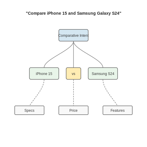
Modern search systems decompose queries into structured semantic representations using techniques like dependency parsing and neural sequence-to-sequence models. Given a query q, the system generates a parse tree T(q) that captures entities, relations, and actions. For example, the query "compare iPhone 15 and Samsung Galaxy S24" would be parsed into a comparative intent structure with two product entities and a comparison operator.
State-of-the-art approaches use transformer-based architectures fine-tuned on query-parse tree pairs, achieving F1 scores above 0.92 on benchmark datasets like ATIS and TOP. The key innovation lies in joint training of token-level and span-level representations to handle nested query structures.
Query Expansion Techniques
Pseudo-relevance feedback (PRF) remains a dominant approach for query expansion, but neural methods have surpassed traditional Rocchio algorithms. The expansion terms E(q) are selected based on:
where R is the top-k retrieved documents and τ is a relevance threshold. BERT-based cross-encoders now achieve superior performance by modeling term importance in context, with expansions improving nDCG by 15-20% on TREC benchmarks.
Knowledge-Augmented Expansion
External knowledge graphs (e.g., Wikidata, ConceptNet) provide ontological relationships for expansion. The expansion score combines:
where simKG measures conceptual relatedness through graph walks. Recent work on dense knowledge graph embeddings (e.g., ComplEx, RotatE) has reduced the latency of such expansions from 500ms to under 50ms per query.
Neural Query Rewriting
Sequence-to-sequence models like T5 and BART generate fluent query rewrites by learning from search session logs. The rewriting objective maximizes:
where (q,q') are observed query reformulation pairs. Deployed systems use constrained beam search to ensure rewrites maintain the original intent while improving clarity, with ablation studies showing 28% reduction in subsequent refinement queries.
Multimodal Query Understanding
For voice and image-augmented queries, systems fuse modalities through cross-attention mechanisms:
CLIP-style contrastive pretraining has proven particularly effective, reducing multimodal query misunderstanding errors by 40% in production systems compared to late fusion baselines.
5. Handling Bias and Fairness in Reranking
5.1 Handling Bias and Fairness in Reranking
Sources of Bias in Reranking Models
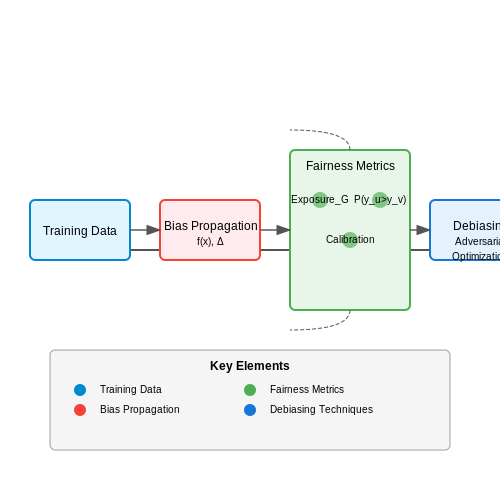
Reranking models inherit biases from multiple sources, including training data, feature selection, and user interaction feedback loops. Training data often reflects historical biases present in human-labeled datasets or click logs, where certain demographics or viewpoints are overrepresented. Feature selection introduces bias when the engineered features correlate with protected attributes like gender, race, or socioeconomic status. User feedback loops exacerbate bias when the model's outputs influence future training data, creating a self-reinforcing cycle.
Mathematically, we can model bias propagation through the ranking function. Let f(x) be the scoring function, and D the training distribution. The expected score disparity between groups A and B is:
Quantifying Fairness in Rankings
Fairness metrics for reranking extend beyond classification fairness to account for position-sensitive outcomes. Three principal metrics are:
- Exposure Fairness: Measures disparity in average visibility across groups. For a ranking of length k:
where γj represents position bias (typically 1/log(1+j)).
- Pairwise Fairness: Ensures consistent pairwise accuracy across groups:
- Calibration Fairness: Requires predicted relevance distributions to match across groups when conditioned on true relevance.
Debiasing Techniques
Pre-processing Methods
Data reweighting adjusts sample importance to balance group representation. For protected attribute a with distribution P(a), weights w = 1/P(a) normalize group prevalence. Adversarial debiasing trains an auxiliary classifier to predict the protected attribute from embeddings, with gradients inverted to remove sensitive information:
In-processing Methods
Constrained optimization formulates fairness as regularization terms. The Lagrangian approach solves:
where Mj are fairness constraints. Counterfactual fairness enforces invariance to protected attribute perturbations through causal modeling.
Post-processing Methods
Fair ranking algorithms like FA*IR modify output rankings to satisfy statistical parity. The deterministic variant ensures at least k·p items from protected group appear in top k, where p is the minimum proportion. Probabilistic versions sample rankings from a distribution meeting fairness constraints.
Tradeoffs and Practical Considerations
The fairness-utility tradeoff surface follows a Pareto frontier, where improving fairness metrics typically reduces ranking quality. The tradeoff can be quantified as the normalized drop in NDCG versus improvement in fairness metric. In production systems, A/B testing frameworks should monitor both engagement metrics and fairness indicators across user segments. Dynamic approaches adapt fairness constraints based on real-time disparity measurements.
Position bias interacts with fairness interventions - demoting overexposed groups in top positions may inadvertently suppress them in subsequent positions due to reduced exploration. Multi-objective optimization frameworks like those using the Chebyshev scalarization method balance these competing requirements:
where fj are objective functions (e.g., NDCG, exposure disparity) and zj* ideal values.
5.2 Scalability and Efficiency Concerns
Reranking models in large-scale information retrieval systems face significant computational challenges as the number of documents grows. The time complexity of reranking n documents for a query is typically O(n) for lightweight models but can escalate to O(n2) or worse for pairwise or listwise approaches. When dealing with web-scale corpora where n may exceed 106 documents per query, this becomes computationally prohibitive.
Approximation Techniques
To maintain practical runtime, most production systems employ approximation strategies:
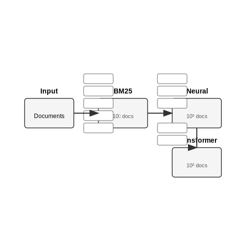
- Cascade architectures progressively apply more expensive models to smaller subsets, e.g., BM25 → neural first-stage → transformer reranker
- Early stopping in transformer inference by terminating low-scoring sequences
- Distillation of large rerankers into smaller student models
where ni is the number of documents processed by stage i with average latency ti.
Hardware Considerations
Modern reranking systems exploit GPU/TPU parallelism through:
- Batch processing of documents across queries
- Mixed-precision inference (FP16/INT8 quantization)
- Model partitioning across multiple devices
The memory footprint of transformer-based rerankers follows:
where d is embedding dimension and L is sequence length, creating practical limits on batch sizes.
Indexing Optimizations
Advanced retrieval-augmented systems pre-compute document representations using:
- Maximum Inner Product Search (MIPS) data structures
- Locality-Sensitive Hashing (LSH) for approximate similarity
- Product quantization of dense embeddings
The tradeoff between recall and computational cost follows:
where p is the probability of a hash collision and k is the number of hash tables.
Distributed Computation
For web-scale deployment, systems employ:
- Sharded document collections with query broadcasting
- Asynchronous result aggregation
- Specialized hardware like ANN accelerators
The latency scalability follows Amdahl's law:
where α is the parallelizable fraction and s is the number of shards.
5.3 Emerging Trends in Relevance Modeling
Neural Reranking with Transformer Architectures
The shift from traditional lexical matching to neural reranking has been accelerated by transformer-based models like BERT, T5, and GPT-3. These models leverage self-attention mechanisms to capture contextual relationships between query-document pairs. The relevance score s(q, d) is computed as:
where W is a learned projection matrix and [q; d] denotes concatenated query-document embeddings. Cross-encoder architectures achieve state-of-the-art performance by jointly encoding the pair, while bi-encoders enable efficient approximate nearest neighbor search through pre-computed document embeddings.
Contrastive Learning for Dense Retrieval
Recent work replaces traditional negative sampling with in-batch contrastive learning, where positive pairs (q, d⁺) are contrasted against hard negatives (q, d⁻) within the same batch. The loss function optimizes:
Key innovations include ANCE (Approximate Nearest Neighbor Negative Contrastive Learning) and COCO-DR, which generate hard negatives through asynchronous refreshes of the document index during training.
Multi-Modal Relevance Modeling
Modern systems increasingly process heterogeneous data types:
- CLIP-style models align image-text embeddings for cross-modal retrieval
- Graph neural networks incorporate knowledge graph relations into document scoring
- Multimodal BERT fuses text, image patches, and tabular data through modality-specific encoders
The relevance function extends to:
where M denotes modalities and λ_m are learned mixture weights.
Differentiable Search Indexing
Pioneered by models like DSI and NCI, this paradigm unifies retrieval and ranking into a single neural network that directly maps queries to document identifiers. The architecture:
- Encodes queries into latent representations
- Generates document ID distributions via sequence-to-sequence modeling
- Optimizes end-to-end using teacher forcing with ground truth (q, docID) pairs
Ethical Considerations in Neural Ranking
Emerging challenges require attention:
- Bias mitigation: Adversarial debiasing techniques for demographic fairness
- Explainability: Attention visualization and counterfactual explanations
- Privacy-preserving retrieval: Federated learning with secure aggregation
Recent work introduces fairness constraints into the ranking objective:
where z represents protected attributes and β controls the fairness-utility tradeoff.

6. Key Research Papers and Books
6.1 Key Research Papers and Books
- Re-ranking Search results based on Relevancy weight: Approach and ... — Re-ranking not only improves the search engine's hit rate but also helps the user to find the desired material more quickly.Further this paper performs the evaluation of the model by comparing it earlier search results. The system proved to be efficient and secure. ... Electronic ISBN: 978-1-6654-3656-4 Print on Demand(PoD) ISBN: ...
- MRR: an unsupervised algorithm to rank reviews by relevance - ResearchGate — In a few papers, unsupervised learning based approaches have been used to rank reviews based on their helpfulness or relevance (Tsur and Rappoport, 2006;Wu et al., 2011; Woloszyn et al., 2017). It ...
- Relevance Ranking for Vertical Search Engines - O'Reilly Media — Book description. In plain, uncomplicated language, and using detailed examples to explain the key concepts, models, and algorithms in vertical search ranking, Relevance Ranking for Vertical Search Engines teaches readers how to manipulate ranking algorithms to achieve better results in real-world applications. This reference book for professionals covers concepts and theories from the ...
- PDF GRN: Generative Rerank Network for Context-wise Recommendation - arXiv.org — strategy based reranking methods to the context-wise reranking strategy. There are also some works [7, 12, 13, 29] focusing on making the trade-off between relevance and diversity in the reranking stage. Different from these works, GRN is an end-to-end context-wise reranking framework, which may automatically generate diverse
- Re-considering and Re-ranking | SpringerLink — PRM is a re-ranking model used by Alibaba in Taobao's recommendations, which uses Transformer to model the mutual influence between item lists and generate the final re-ranking results. As shown in Fig. 6.5 , the PRM model consists of three parts: the input layer, the encoding layer, and the output layer.
- GRN: Generative Rerank Network for Context-wise Recommendation — Reranking is attracting incremental attention in the recommender systems, which rearranges the input ranking list into the final rank-ing list to better meet user demands. Most existing methods greedily rerank candidates through the rating scores from point-wise or list-wise models. Despite effectiveness, neglecting the mutual influence between each item and its contexts in the final ranking ...
- Ranking 'by Relevance' in Academic Literature Searches: Prevalence ... — The concept of ranking 'by relevance' arose from challenges in accessing increasingly large amounts of digital data more generally (König and Rasch 2014).Yet, it is important to consider within the context of academic literature searches, in order to interrogate the challenges of outsourcing academic labour to algorithms.
- PDF Document reRanking using GAT-Cross Encoder - papers.dice-research.org — Document re-ranking is a crucial post-processing step, focused on reordering an initial list of documents to better meet the information needs associated with a user query. In this paper, we explore the application of graph attention networks to enhance the re-ranking process in information retrieval systems. Traditional meth-
- Graph-Based Re-ranking: - arXiv.org — Retrieval Augmented Generation (RAG) is an established research area that combines pretrained parametric and non-parametric memory for downstream language generation Lewis et al. ().Recently, there has been an emergence of using Knowledge Graphs as the external non-parametric datastore, in which structural information is queried to capture relational knowledge Dong et al. ().
- Incorporating rich features to boost information retrieval performance ... — Research highlights We propose a regression-based re-ranking framework that can take into account rich features for boosting information retrieval (IR) performance. A set of salient features that may affect IR performance are investigated. Extensive experimental results on four standard test collections show that our proposed approach can significantly improve the retrieval performance over ...
6.2 Open Datasets and Benchmarks
- Azure AI Search: Outperforming vector search with hybrid retrieval and ... — Table 1: Retrieval comparison using Azure AI Search in various retrieval modes on customer and academic benchmarks.See §6.1 How we generated the numbers in this post and §6.2 Search and Dataset configuration for Table 1 for the setup and measurement details.. 3. Hybrid Retrieval brings out the best of Keyword and Vector Search. Keyword and vector retrieval tackle search from different ...
- arXiv:1903.06902v3 [cs.IR] 27 Jun 2019 — IR community [10, 35]. Standard benchmark datasets [36, 37], evaluation tasks [38], and open-source toolkits [39] have been created to facilitate research and rigorous comparison. Meanwhile, in industry, we have also seen models such as DSSM put into a wide range of practical usage in the enterprise [40]. Neural
- Rankify: A Comprehensive Python Toolkit for Retrieval, Re-Ranking, and ... — tionally, retrieval and re-ranking datasets are scattered across differ-ent sources, complicating evaluation and comparison. To address these challenges, we introduce Rankify, an open-source frame-work that unifies retrieval, re-ranking, and RAG into a modular and extensible ecosystem (logo shown in Figure 1). Rankify sup-
- RankVicuna: Zero-Shot Listwise Document Reranking - ar5iv — RankVicuna provides exactly this: To our knowledge, we present the first open-source large language model for zero-shot listwise document reranking. Experimental validation on test collections from the TREC 2019 and 2020 Deep Learning Tracks Craswell et al. ( 2020 , 2021 ) shows that the effectiveness of our model is on par with zero-shot ...
- (PDF) Modeling Relevance Ranking under the Pre-training ... - ResearchGate — Modeling Relevance Ranking under the Pre-training and Fine-tuning Paradigm Table 3: Impacts of the handcrafted learning-to-rank features at the ne-tuningstage. MQ2007 MQ2008 TREC19
- Advanced RAG 04: Re-ranking - Medium — Using re-ranking model as reranker. The re-ranking model, unlike the embedding model, takes query and contexts as inputs and directly outputs similarity scores instead of embeddings. It is important to note that the re-ranking model is optimized using cross-entropy loss, allowing for relevance scores that are not limited to a specific range and ...
- From Good to Great: Using Reranking Models to Perfect Your RAGs — Recent studies on popular datasets such as BEIR and CodeSearchNet offer a detailed look at how different reranking models perform across various tasks. Let's explore these benchmarks to see how ...
- Re-ranking - Dify Docs — Why is Re-ranking Needed? Hybrid search can leverage the strengths of different retrieval technologies to achieve better recall results. However, the query results from different retrieval modes need to be merged and normalized (converting data to a uniform standard range or distribution for better comparison, analysis, and processing) before being provided to the large model together.
- A Deep Look into neural ranking models for information retrieval — In more detail, this type of model should optimize two objectives: (i) a relevance objective that maximizes the effectiveness of the model in terms of the retrieval performance, and (ii) a sparsity objective that is equivalent to minimizing L 0 of the query and document representations. SNRM has shown superior performance compared to ...
- T2Ranking: A large-scale Chinese Benchmark for Passage Ranking — FR(SR): First (Second)-stage of passage ranking, i.e., passage Retrieval (Re-ranking). Examples for annotation of query-passage pair. Performance of retrieval models on the test set of T 2 Ranking.
6.3 Tools and Libraries for Implementation
- The Rocchio algorithm for relevance feedback - Stanford University — The Rocchio Algorithm is the classic algorithm for implementing relevance feedback. It models a way of incorporating relevance feedback information into the vector space model of Section 6.3. Figure 9.3: The Rocchio optimal query for separating relevant and nonrelevant documents. Subsections.
- Rank1: Test-Time Compute for Reranking in Information Retrieval — limits the model's ability to be precise. Thus, our work focuses on bringing test-time compute to IR in a reranking setting, where the model needs to compute the relevance of an initial top-k candidates. To accomplish this goal, we sample 635,000 examples of R1's thought process on the MS MARCO dataset (Nguyen et al.,2016).
- Reranking. A Reranker is a language model that… | by Sascha Heyer ... — A Ranker is a language model that computes a relevance score using a document and a query. The score computed is high for a document with a contextually relevant query document pair and low for ...
- Advanced RAG 04: Re-ranking - Medium — Using re-ranking model as reranker. The re-ranking model, unlike the embedding model, takes query and contexts as inputs and directly outputs similarity scores instead of embeddings. It is important to note that the re-ranking model is optimized using cross-entropy loss, allowing for relevance scores that are not limited to a specific range and ...
- Learning to Rank: A Complete Guide to Ranking using Machine Learning ... — Ranking models typically work by predicting a relevance score s = f(x) for each input x = (q, d) where q is a query and d is a document. Once we have the relevance of each document, we can sort (i.e. rank) the documents according to those scores. Ranking models rely on a scoring function. (Image by author)
- Re-ranking in RAG: Improve Retrieval with Top Techniques — Re-ranking addresses challenges like retrieval noise and query ambiguity by employing advanced scoring mechanisms to filter out irrelevant or low-quality documents, ensuring that only the most relevant information is passed to the generation model. For retrieval noise, re-ranking models evaluate the semantic alignment of documents with the ...
- Introducing Learning To Rank (LTR) in Elasticsearch — Typically, the model is used as a second stage re-ranker, to improve the relevance of search results returned by a simpler, first stage retrieval algorithm. This blog post will explain how this new feature can help in improving your document ranking in text search and how to implement it in Elasticsearch.
- Mastering Re-Ranking for Superior LLM RAG Retrieval: A ... - Medium — Incorporating Re-Ranking: Integrate the trained re-ranking model into the existing LLM-based retrieval system, ensuring compatibility and seamless operation within the retrieval pipeline. 2.
- PDF The BERT Ranking Paradigm: Training Strategies Evaluated - ru — bene cial to apply transfer learning by training the model on a closely related task [22, 10, 1]. The following paragraph presents a set of research questions based on the fact that the Cran eld collection has multiple relevance labels, i.e., for each relevant document is has a relevance score, more details will be discussed in Section 1.4.
- A Practical Guide to Implementing Enhanced RAG with Re-Ranking — Re-ranking is a technique to enhance the retrieval process. It refines the initial set of retrieved documents. This ensures that the most relevant documents are prioritized for the generation of ...