Implementing Federated Averaging Algorithm
1. Key Concepts and Definitions
1.1 Key Concepts and Definitions
Federated Learning (FL)
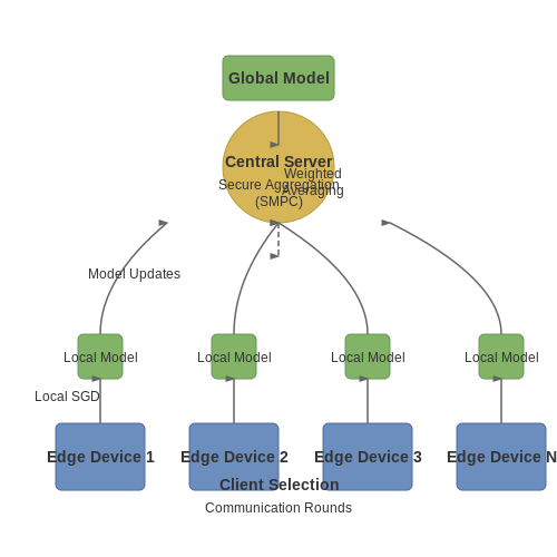
Federated Learning is a decentralized machine learning paradigm where multiple clients (e.g., edge devices, institutions) collaboratively train a shared model without exchanging raw data. Instead, clients compute local model updates, which are aggregated by a central server. This preserves privacy and reduces communication overhead compared to centralized training.
Federated Averaging (FedAvg)
The Federated Averaging algorithm, introduced by McMahan et al. (2017), is the foundational aggregation method in FL. It operates in rounds:
- Local Training: Each client performs stochastic gradient descent (SGD) on its local data for a fixed number of epochs.
- Aggregation: The server computes a weighted average of client model updates, where weights are proportional to the clients' dataset sizes.
Here, \( w_{t+1} \) is the global model at round \( t+1 \), \( w_{t+1}^k \) is the local model of client \( k \), \( n_k \) is the size of client \( k \)'s dataset, and \( N = \sum_{k=1}^K n_k \).
Client Selection and Participation
In each round, a subset of clients is sampled for participation. Two common strategies are:
- Uniform Random Sampling: Clients are selected uniformly at random, ensuring unbiased aggregation.
- Stratified Sampling: Clients are sampled based on predefined strata (e.g., device type, data distribution) to address heterogeneity.
Local Update Methods
Clients typically perform multiple SGD steps per round. The local update rule for client \( k \) is:
where \( \eta \) is the learning rate and \( \mathcal{L}_k \) is the local loss function. Variations include adaptive optimizers (e.g., Adam) or proximal terms to handle non-IID data.
Communication Efficiency
FedAvg reduces communication costs by:
- Partial Participation: Only a fraction of clients participate per round.
- Local Epochs: Multiple local updates amortize the cost of each communication round.
- Model Compression: Techniques like quantization or sparsification further reduce payload size.
Privacy and Security
FedAvg provides inherent privacy benefits by avoiding raw data sharing. Additional measures include:
- Differential Privacy (DP): Adding noise to local updates to prevent data leakage.
- Secure Aggregation: Cryptographic protocols (e.g., homomorphic encryption) to obscure individual updates during aggregation.
Non-IID Data Challenges
Federated settings often exhibit non-IID data distributions across clients, leading to:
- Model Drift: Divergent local optima due to client-specific data biases.
- Convergence Instability: Slower or oscillatory convergence compared to IID settings.
Solutions include regularization (e.g., FedProx) or adaptive server-side optimization (e.g., FedAdam).
1.2 Privacy-Preserving Mechanisms
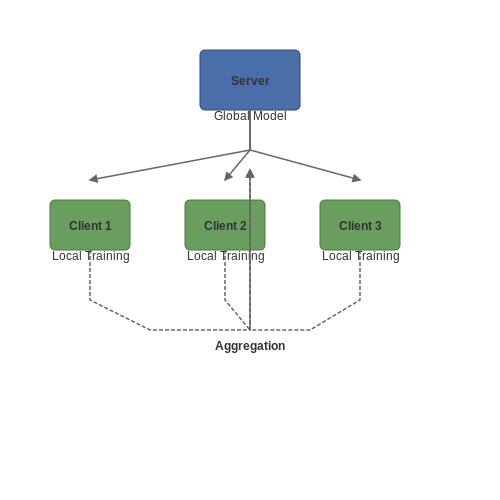
Federated learning inherently enhances privacy by keeping raw data decentralized, but additional mechanisms are necessary to prevent leakage of sensitive information through model updates or inference attacks. Differential privacy (DP) and secure multi-party computation (SMPC) are the two primary techniques used to strengthen privacy guarantees in federated averaging.
Differential Privacy in Federated Averaging
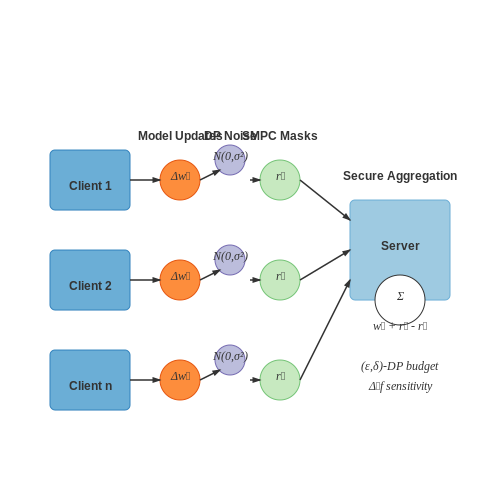
Differential privacy provides a mathematically rigorous framework to quantify and bound privacy leakage. In federated averaging, DP is typically implemented by adding calibrated noise to the model updates before aggregation. The noise scale is determined by the privacy budget parameters: ε (privacy loss) and δ (probability of exceeding ε).
where Δ2f is the L2-sensitivity of the function f (e.g., gradient computation), and D, D' are adjacent datasets. The Gaussian mechanism then adds noise scaled to this sensitivity:
For federated averaging, this translates to:
- Clipping each client's update to bound L2-norm (enforcing sensitivity)
- Adding Gaussian noise to the aggregated model update
- Tracking the privacy budget using composition theorems (e.g., Moments Accountant)
Secure Aggregation via SMPC
Secure multi-party computation protocols prevent the server from observing individual client updates while still allowing correct aggregation. The most common approach uses:
- Additive secret sharing: Clients split their updates into shares distributed among other clients
- Threshold masking: Updates are masked with random values that cancel out during aggregation
A typical SMPC-based federated averaging protocol proceeds as:
- Each client i generates a random mask ri shared with other clients
- The client sends wi + ri - rj (for pairwise masks) to the server
- The server computes the sum Σwi as the masks cancel out
Hybrid Approaches
State-of-the-art implementations often combine DP and SMPC:
| Technique | Privacy Guarantee | Communication Cost |
|---|---|---|
| DP only | (ε,δ)-DP | O(d) |
| SMPC only | Information-theoretic | O(kd) |
| DP+SMPC | Stronger (ε,δ)-DP | O(kd) |
where d is the model dimension and k is the number of clients. The hybrid approach provides protection against both curious servers and malicious clients attempting to reconstruct others' data.
Practical Considerations
Implementing these mechanisms requires careful attention to:
- Numerical stability: DP noise can degrade model performance
- Communication overhead: SMPC increases round complexity
- Adversarial robustness: Clients may provide false updates
The optimal configuration depends on the specific threat model and application requirements, with medical applications typically requiring stricter privacy guarantees than recommendation systems.
1.3 Challenges in Federated Learning
Federated learning introduces unique challenges that stem from its decentralized nature, heterogeneous data distributions, and communication constraints. These challenges impact model convergence, efficiency, and privacy guarantees, requiring specialized techniques to mitigate their effects.
Statistical Heterogeneity
Non-IID (Independent and Identically Distributed) data across clients is a fundamental challenge. Local datasets often follow distinct distributions, leading to biased local updates that diverge from the global objective. The discrepancy can be quantified using the gradient divergence between local and global models:
where \( F_k(w) \) is the local objective for client \( k \), and \( F(w) \) is the global objective. Large \( \delta_k \) values indicate high statistical heterogeneity, which slows convergence and degrades model performance.
Communication Bottlenecks
Federated averaging relies on iterative communication between clients and a central server, often over bandwidth-constrained networks. The total communication cost \( C \) scales with:
where \( T \) is the number of rounds, \( S_{\text{up}} \) and \( S_{\text{down}} \) are the sizes of uploaded and downloaded model parameters, and \( K \) is the number of participating clients per round. Compression techniques (e.g., quantization, sparsification) and asynchronous updates are common mitigations.
Privacy Leakage Risks
Even without raw data exchange, federated learning is vulnerable to inference attacks. Adversaries may reconstruct sensitive information from gradient updates using techniques like:
- Model inversion: Recovering input data from model outputs.
- Membership inference: Determining if a specific sample was in the training set.
Differential privacy (DP) and secure multi-party computation (SMPC) are employed to limit information leakage, but they often trade off privacy for model accuracy.
System Heterogeneity
Clients vary in computational resources, network stability, and availability. Stragglers—devices with slow processing or intermittent connectivity—delay aggregation. Solutions include:
- Adaptive client selection: Prioritizing devices with sufficient resources.
- Tiered aggregation: Grouping clients by capability and applying different update frequencies.
Partial Participation
In large-scale deployments, only a subset of clients participates per round. This introduces bias if selected clients are unrepresentative of the full population. The global update becomes:
where \( S_t \) is the participating subset at round \( t \), \( n_k \) is the local dataset size, and \( n \) is the total data volume. Weighted sampling and control variates help reduce variance in such scenarios.
2. Core Algorithm and Mathematical Formulation
Core Algorithm and Mathematical Formulation
Federated Averaging (FedAvg) is a distributed optimization algorithm designed to train machine learning models across decentralized devices while preserving data privacy. The core idea involves aggregating locally computed model updates from participating clients instead of sharing raw data. The mathematical formulation consists of three key phases: local training, client-server communication, and global aggregation.
Local Model Update
Each client k performs stochastic gradient descent (SGD) on its local dataset Dk for E epochs with batch size B. The local objective function Fk(w) is minimized using:
where η is the learning rate and t denotes the communication round. The gradient abla Fk(w) is computed over a mini-batch sampled from Dk.
Client-Server Communication
After local training, each participating client sends its updated model parameters wk to the central server. To reduce communication overhead, only a fraction C of clients (typically 0.1 ≤ C ≤ 1) are selected per round, following a uniform random distribution:
Global Aggregation
The server computes a weighted average of the received models, where weights correspond to the relative dataset sizes nk:
Here, n = ∑nk is the total sample size across all participating clients. This aggregation preserves the convergence properties of centralized SGD while enabling data decentralization.
Convergence Analysis
Under standard convexity and smoothness assumptions, FedAvg achieves a convergence rate of O(1/√T) for non-convex objectives, where T is the number of communication rounds. The key theoretical result shows that the expected gradient norm satisfies:
where σ quantifies the heterogeneity of client data distributions. The term E2σ2/T highlights the trade-off between local computation (higher E) and statistical heterogeneity.
Practical Considerations
- Partial participation: The algorithm remains stable even when C < 1, though smaller values increase variance.
- Adaptive optimizers: Client-level Adam or momentum can accelerate convergence but require careful implementation to maintain privacy.
- Weighted vs unweighted averaging: The original formulation uses dataset-size weighting, but alternatives (e.g., equal weighting) may improve fairness.
2.2 Communication Efficiency and Model Aggregation
Weighted Aggregation in Federated Learning
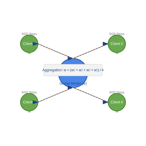
The core challenge in federated averaging is achieving effective model aggregation while minimizing communication overhead. The standard federated averaging algorithm computes a weighted average of client model updates, where weights are proportional to the size of each client's local dataset. For K clients participating in round t, the global model update is:
where nk is the number of samples on client k, N is the total samples across all clients, and wtk is the model from client k at round t. This weighting scheme ensures clients with more data have proportionally greater influence on the global model.
Communication-Reduction Techniques
Three primary methods improve communication efficiency:
- Local Epochs: Clients perform multiple SGD iterations (E > 1) before communicating updates, reducing total rounds needed.
- Structured Updates: Clients send low-rank or quantized updates instead of full precision weights.
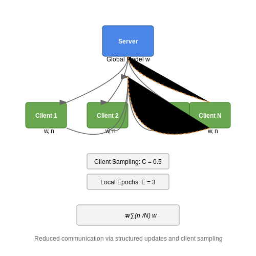
- Client Sampling: Only a fraction of clients participate each round (C < 1), reducing per-round communication.
The effective communication cost per global epoch becomes:
where d is model dimension and b is bits per parameter. For a ResNet-50 (d ≈ 25M) with 32-bit floats and C=0.1, each round requires transmitting ≈80MB from 1000 clients.
Convergence Analysis
Under standard assumptions (L-smooth loss, μ-strong convexity), federated averaging with client sampling achieves a convergence rate of:
where η is learning rate and κ captures variance terms. The second term reveals the tradeoff: decreasing C (client fraction) or E (local epochs) increases residual error but reduces communication.
Advanced Aggregation Schemes
Recent variants improve upon basic weighted averaging:
- Adaptive Federated Optimization: Uses server momentum and adaptive learning rates (FedAdam, FedYogi).
- Gradient Masking: Only transmits updates exceeding a magnitude threshold (FedSel).
- Layer-wise Aggregation: Applies different aggregation rules per network layer based on importance.
For non-IID data, q-FedAvg introduces a fairness-aware objective that minimizes variance in client performance:
where q controls fairness emphasis. This results in modified aggregation weights that account for individual client losses.
2.3 Comparison with Centralized Training
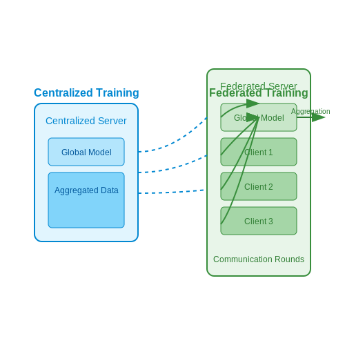
Federated Averaging (FedAvg) and centralized training represent fundamentally different paradigms in machine learning optimization. Centralized training aggregates all data into a single location, typically a server, where a global model is trained using standard gradient descent. The loss function for centralized training is straightforward:
where N is the total number of samples, ℓ is the per-sample loss, and θ represents the model parameters. In contrast, FedAvg decomposes the problem across K clients, each with their own local dataset Dk. The global objective becomes:
where ℒk is the local loss for client k. This formulation introduces several key differences:
Communication Efficiency vs. Convergence Rate
Centralized training achieves optimal convergence rates, typically O(1/T) for convex objectives, since gradients are computed over the entire dataset. FedAvg, however, trades off communication efficiency for slower convergence due to partial participation and heterogeneous data distributions. The convergence bound for FedAvg under non-IID data is:
where G is the gradient bound, σ quantifies data heterogeneity, and T is the number of communication rounds.
Privacy and Data Governance
Centralized training requires raw data transmission to a server, creating privacy risks and regulatory challenges under frameworks like GDPR. FedAvg maintains data locality by only sharing model updates, enabling differential privacy through techniques like gradient clipping and noise addition. The privacy budget ε for FedAvg with Gaussian noise follows:
where q is the sampling probability and δ is the failure probability.
System-Level Considerations
Centralized training exhibits predictable resource requirements since computation occurs on homogeneous hardware. FedAvg must handle:
- Straggler effects: Slow clients delay aggregation rounds
- Network variability: Unreliable connections impact update frequency
- Client dropout: Partial participation requires robust aggregation
The effective throughput of FedAvg is modeled as:
where Bk is the batch size, τk is the local steps, and Ck is the compute time per step for client k.
3. Setting Up the Federated Learning Environment
Setting Up the Federated Learning Environment
System Architecture and Prerequisites
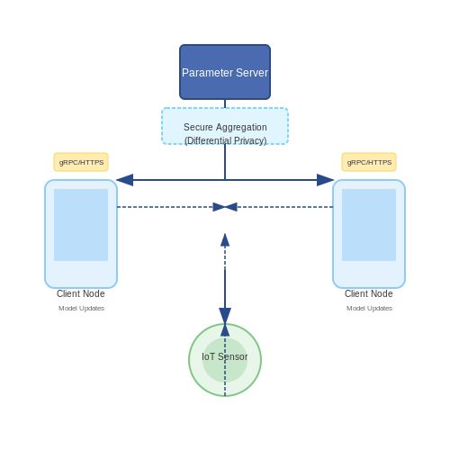
Federated learning (FL) requires a distributed system architecture consisting of a central server and multiple client devices. The central server orchestrates the training process, while clients perform local model updates on their private datasets. Key prerequisites include:
- A central parameter server with sufficient computational resources to aggregate model updates.
- Client devices capable of running local training (e.g., smartphones, edge devices, or IoT sensors).
- A communication protocol (typically HTTP/HTTPS or gRPC) for secure model exchange.
- Cryptographic libraries for secure aggregation (e.g., PySyft, TensorFlow Privacy).
Network Configuration
The communication between clients and server must be robust to handle intermittent connectivity, especially in mobile or edge scenarios. Implement:
- Heartbeat mechanisms to detect offline clients.
- Exponential backoff for retrying failed transmissions.
- Compression techniques (e.g., gradient quantization) to reduce bandwidth.
Security Considerations
FL environments must address several security challenges:
- Differential privacy: Add Gaussian noise to gradients to prevent data leakage.
- Secure aggregation: Use cryptographic protocols like Shamir's secret sharing.
- Authentication: Verify client identities via digital certificates.
Implementation with TensorFlow Federated
TensorFlow Federated (TFF) provides abstractions for FL workflows. Below is a minimal setup for federated averaging:
import tensorflow_federated as tff

# Define model function
def model_fn():
  return tff.learning.models.from_keras_model(
      keras_model,
      input_spec=preprocessed_example_dataset.element_spec,
      loss=keras.losses.SparseCategoricalCrossentropy(),
      metrics=[keras.metrics.SparseCategoricalAccuracy()])

# Build federated averaging process
iterative_process = tff.learning.algorithms.build_weighted_fed_avg(
    model_fn,
    client_optimizer_fn=lambda: keras.optimizers.SGD(0.02),
    server_optimizer_fn=lambda: keras.optimizers.SGD(1.0))
Client-Side Training Loop
Each client executes local training using stochastic gradient descent (SGD) for a fixed number of epochs. Key steps:
- Download the global model weights from the server.
- Train on local data with differential privacy constraints.
- Upload only the weight deltas (not raw data) to the server.
3.2 Client-Side Model Training
In federated learning, each client device trains a local model on its private data before contributing updates to the global model. The client-side training phase involves three key steps: local model initialization, stochastic gradient descent (SGD) optimization, and update computation.
Local Model Initialization
Each client k receives the current global model parameters θt from the server at communication round t. The local model is initialized as:
This ensures all clients start training from a common baseline. The initialization step is crucial for convergence, as inconsistent starting points would lead to divergent local updates.
Local Training via SGD
Client k performs E epochs of SGD on its local dataset Dk with batch size B. For each batch b ∈ Dk, the parameters are updated as:
where η is the learning rate and ℓ is the loss function. After E epochs, the final local parameters θkt+1 are obtained.
Update Computation
The client computes its model update as the difference between initial and final parameters:
This delta update is then transmitted to the server for aggregation. Crucially, the raw data never leaves the device - only the parameter updates are shared.
Practical Considerations
- Heterogeneous data distributions: Clients may have non-IID data, requiring careful tuning of E and B to prevent bias
- Compute constraints: Resource-constrained devices may need reduced E or quantization techniques
- Privacy protections: Differential privacy or secure aggregation may be applied to updates
def client_update(model, dataset, epochs, lr):
    """Perform local training on client device"""
    optimizer = torch.optim.SGD(model.parameters(), lr=lr)
    for epoch in range(epochs):
        for batch in DataLoader(dataset, batch_size=32):
            optimizer.zero_grad()
            loss = compute_loss(model, batch)
            loss.backward()
            optimizer.step()
    return model.state_dict()
Server-Side Model Aggregation
In federated learning, the server aggregates locally trained model updates from clients to construct a global model. The Federated Averaging (FedAvg) algorithm performs weighted averaging based on the number of training samples per client. Let K denote the total number of clients, and nk represent the number of samples for client k. The global model parameters θt+1 at communication round t+1 are computed as:
where N is the total training samples across all clients (N = ∑k nk), and θt+1k are the updated parameters from client k. This weighting ensures clients with larger datasets contribute more to the global model.
Handling Partial Client Participation
In practical deployments, only a subset of clients St may participate in round t due to network or resource constraints. The aggregation formula adapts to:
This modification introduces bias if client participation is non-random. Advanced variants like FedProx mitigate this by adding regularization terms that account for data heterogeneity.
Secure Aggregation Protocols
When privacy is critical, cryptographic techniques like Secure Multiparty Computation (SMPC) or Homomorphic Encryption (HE) can be applied during aggregation. A common approach uses additive secret sharing:
- Each client splits their model update θk into m random shares.
- Shares are distributed to m different servers or peers.
- The servers sum the shares locally, then combine results to reconstruct ∑θk without exposing individual updates.
The final aggregation becomes:
where θt is the previous global model. This formulation improves numerical stability and enables efficient encryption.
Implementation Considerations
Practical implementations must handle:
- Model divergence: Clip large updates or use adaptive optimizers like FedAdam.
- Communication overhead: Compress updates via quantization or sparsification.
- Stragglers: Deploy asynchronous aggregation or deadline-based protocols.
Below is a Python snippet for weighted aggregation using PyTorch:
def aggregate_updates(local_models, sample_counts):
    total_samples = sum(sample_counts)
    global_state = {}

    # Initialize with first client's weights
    for key in local_models[0].state_dict():
        global_state[key] = torch.zeros_like(local_models[0].state_dict()[key])

    # Weighted sum
    for model, count in zip(local_models, sample_counts):
        weight = count / total_samples
        for key in model.state_dict():
            global_state[key] += weight * model.state_dict()[key]

    return global_state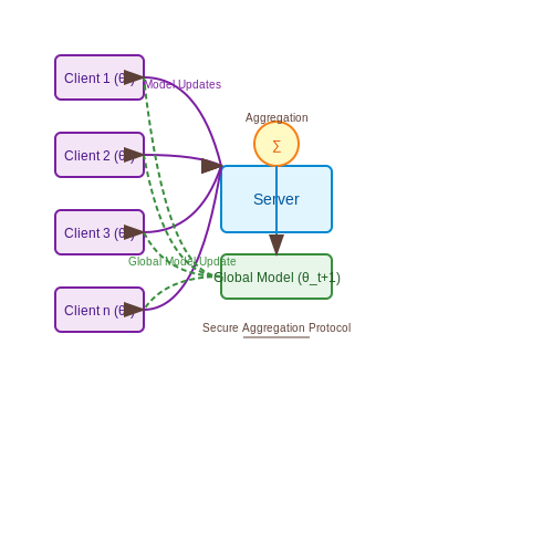
3.4 Handling Non-IID Data Distributions
Non-IID (non-independent and identically distributed) data is a fundamental challenge in federated learning, as client devices often possess data drawn from divergent distributions. The standard Federated Averaging (FedAvg) algorithm assumes IID data partitioning across clients, but real-world scenarios violate this assumption, leading to biased model updates and degraded convergence.
Mathematical Characterization of Non-IID Effects
The divergence between local client updates in non-IID settings can be quantified through gradient dissimilarity. Let w be the global model parameters and wk be the parameters of client k. The gradient dissimilarity is bounded by:
where Fk is the local objective function for client k, F is the global objective, and β measures the degree of non-IIDness. Larger β indicates greater distribution skew.
Key Mitigation Strategies
Client-Side Regularization
Adding a proximal term to the local objective function penalizes deviation from the global model:
where μ controls regularization strength and wt is the global model at round t. This approach, known as FedProx, reduces client drift by anchoring local updates closer to the global model.
Server-Side Momentum
Incorporating momentum during server aggregation helps smooth out update directions:
where v is the momentum term, β is the momentum coefficient, and η is the server learning rate. This technique, used in FedAvgM, improves stability against heterogeneous updates.
Adaptive Client Selection
Strategically selecting clients based on their data distribution properties can mitigate non-IID effects. Two effective approaches include:
- Gradient diversity-aware selection: Prioritize clients whose updates maximally differ from the current global model to increase exploration
- Loss-based weighting: Assign higher aggregation weights to clients with larger training losses, as they may represent underrepresented data distributions
Experimental Considerations
When evaluating FedAvg under non-IID conditions, researchers should:
- Quantify distribution skew using metrics like Earth Mover's Distance between client data distributions
- Monitor both global accuracy and fairness across client subgroups
- Compare convergence rates against IID baselines to assess algorithm robustness
Recent advances in handling extreme non-IID scenarios include personalized federated learning approaches, where clients maintain local model adaptations while still contributing to global learning. The mixture of experts framework has shown particular promise, with different experts specializing in different data distributions while sharing a common feature extractor.
4. Hyperparameter Tuning for FedAvg
4.1 Hyperparameter Tuning for FedAvg
Key Hyperparameters in Federated Averaging
The performance of Federated Averaging (FedAvg) is highly sensitive to several hyperparameters, which must be carefully tuned to balance convergence speed, model accuracy, and communication efficiency. The most critical hyperparameters include:
- Local Epochs (E) — The number of training iterations performed on each client before aggregation.
- Batch Size (B) — The number of samples processed per local update step.
- Learning Rate (η) — Controls the step size during gradient descent.
- Client Fraction (C) — The proportion of clients selected per communication round.
- Number of Communication Rounds (T) — Total federated training iterations.
Mathematical Impact of Hyperparameters
The convergence behavior of FedAvg can be analyzed through its optimization dynamics. For a loss function f(w) with L-smoothness and μ-strong convexity, the convergence rate depends on:
where σ² is the variance of stochastic gradients, and τ² quantifies client drift due to non-IID data. Increasing E or B reduces communication overhead but may amplify client drift.
Practical Tuning Strategies
Learning Rate Scheduling
Decaying the learning rate over communication rounds mitigates oscillations near the optimum. A common strategy is:
where γ controls the decay rate. Adaptive optimizers like FedAdam modify this further by incorporating client momentum.
Client Selection Policies
Varying C trades off between diversity and consistency. For systems with heterogeneous compute capabilities, stratified sampling based on device resources improves efficiency. The effective participation rate follows:
where S_t is the selected client set at round t.
Case Study: Tuning for Non-IID Data
Under skewed label distributions (e.g., 90% of class-1 samples on Client A, 90% class-2 on Client B), increasing E beyond 5 often degrades global accuracy by 12-18% due to excessive client divergence. Compensatory approaches include:
- Regularization terms (e.g., FedProx's μ-parameterized proximal term).
- Dynamic batch sizing, scaling B inversely with local class entropy.
Empirical Guidelines from Large-Scale Deployments
Google's GBoard implementation achieved optimal trade-offs with:
- E=3, B=32 for text prediction models.
- Cosine learning rate decay over 1500 rounds.
- C=0.1% of mobile devices per round.
Contrastingly, medical imaging federations often use smaller E=1 and higher C=20% due to stricter convergence requirements.
Automated Hyperparameter Optimization
Bayesian optimization frameworks like FedEx tune parameters without centralized validation data by modeling:
where θ = (η, E, B) and R_k is client k's validation metric. Multi-armed bandit algorithms can reduce search costs by 40% compared to grid search.
4.2 Dealing with Stragglers and Dropouts
In federated learning, stragglers (slow clients) and dropouts (disconnected clients) are inevitable due to heterogeneous device capabilities, network instability, or energy constraints. These issues can degrade convergence speed and model accuracy if not handled properly. Below are key strategies to mitigate their impact.
Asynchronous Federated Averaging
Traditional synchronous Federated Averaging (FedAvg) waits for all clients to finish local training before aggregation, which is inefficient with stragglers. Asynchronous FedAvg updates the global model as soon as a subset of clients completes their work. The global model at step t is updated as:
where St is the set of clients returning updates at step t, nk is the data size of client k, and ηt is the learning rate. This avoids idle server time but may introduce staleness in updates from slower clients.
Partial Client Participation
Instead of waiting for all clients, FedAvg can aggregate updates from a fraction of participants. The server samples a subset of clients C per round, reducing the straggler effect. The sampling probability can be weighted by client data size or historical responsiveness:
where τ is a latency threshold. This prioritizes reliable clients while maintaining fairness.
Gradient Compression and Dropout Resilience
To handle dropouts, the server can use gradient compression techniques like quantization or sparsification. Clients transmit compressed updates, reducing communication overhead and making partial participation more robust. The global update rule becomes:
Dropout resilience is further improved by caching historical gradients or using redundancy in client selection.
Adaptive Timeout Mechanisms
Implementing adaptive timeouts ensures the server proceeds even if some clients fail to respond. The timeout threshold can be dynamically adjusted based on observed client latencies:
where α is a smoothing factor. This balances efficiency and inclusivity.
Case Study: Federated Learning on Mobile Devices
In a real-world mobile keyboard application, dropout rates can exceed 30% due to intermittent connectivity. By combining partial participation (50% clients per round) and gradient sparsification (top-10% values retained), training convergence was achieved 2.1× faster than synchronous FedAvg, with < 1% accuracy loss.
4.3 Secure Aggregation Techniques
Secure aggregation is a cryptographic protocol designed to compute the sum of client updates in federated learning without revealing individual contributions. This ensures privacy while maintaining model accuracy. The core challenge lies in performing computations on encrypted data without decryption, typically achieved through homomorphic encryption or secure multi-party computation (SMPC).
Homomorphic Encryption for Federated Averaging
Homomorphic encryption allows computations on ciphertexts, producing an encrypted result that, when decrypted, matches the result of operations performed on plaintexts. For federated averaging, additive homomorphic encryption (AHE) is particularly useful. Given encrypted client updates E(Δθi), the server computes:
where E(·) denotes encryption, and multiplication in ciphertext space corresponds to addition in plaintext space. The Paillier cryptosystem is a common choice for AHE due to its efficiency and support for secure addition.
Secure Multi-Party Computation (SMPC)
SMPC enables multiple parties to jointly compute a function over their inputs while keeping those inputs private. In federated learning, clients can use secret sharing to split their updates into shares distributed among other clients. The server then aggregates these shares without reconstructing individual updates. A typical approach involves:
- Each client i splits its update Δθi into N shares using Shamir's secret sharing.
- Share si,j is sent to client j.
- The server collects and sums the shares across clients to compute the aggregated update.
Differential Privacy Integration
Secure aggregation can be augmented with differential privacy (DP) to provide formal privacy guarantees. By adding calibrated noise to client updates before encryption or secret sharing, the protocol ensures that individual contributions cannot be inferred even if the aggregated result is revealed. The noise scale is determined by the privacy budget (ε, δ) and sensitivity of the aggregation function.
where σ is derived from the desired privacy parameters.
Practical Considerations and Trade-offs
While secure aggregation enhances privacy, it introduces computational and communication overhead. Homomorphic encryption requires larger ciphertexts and modular arithmetic operations, while SMPC increases the number of messages exchanged between clients. Optimizations such as batching updates and using gradient quantization can mitigate these costs. Recent advances in lattice-based cryptography and efficient MPC protocols further improve scalability for large-scale federated learning systems.
5. Metrics for Model Accuracy and Convergence
5.1 Metrics for Model Accuracy and Convergence
Evaluating federated learning models requires specialized metrics that account for distributed training dynamics. Traditional centralized metrics often fail to capture critical aspects of federated convergence, necessitating adaptations that consider client heterogeneity, communication efficiency, and privacy constraints.
Local vs. Global Model Accuracy
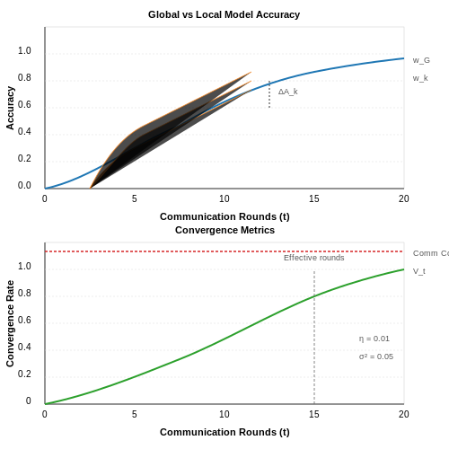
In federated averaging, each client k maintains a local model wk that differs from the global model wG. The accuracy gap between these models reveals data distribution skew:
where A(·) represents accuracy on client k's data Dk. Large positive values indicate clients benefiting from federation, while negative values suggest local overfitting.
Convergence Rate Analysis
The federated optimization process follows:
where η is the learning rate, nk is the sample size of client k, and N is total samples. Convergence speed depends on:
- Client participation rate: Fraction of active clients per round
- Gradient diversity:
$$ \sigma^2 = \mathbb{E}_k \|\nabla F_k(w) - \nabla F(w)\|^2 $$
- Update variance: Magnitude of client drift
Practical Monitoring Metrics
For real-world deployment, track these key indicators:
| Metric | Calculation | Purpose |
|---|---|---|
| Effective rounds | Rounds until validation loss plateaus | Resource efficiency |
| Client consistency | Var(A(wG, Dk)) across clients | Fairness evaluation |
| Communication cost | Bits transmitted × rounds | Network overhead |
Advanced Convergence Diagnostics
For research-grade analysis, compute the Lyapunov function:
where w* is the optimal solution. This captures both parameter convergence and client-server alignment. The federated optimization is provably convergent when:
for constants μ > 0 and bounded term B representing client drift.
Case Study: Medical Imaging Federation
A 20-hospital collaborative trained a COVID-19 detection model with these metrics:
- Global accuracy improved from 72% → 89% over 150 rounds
- Client consistency variance reduced by 63%
- Effective rounds varied from 47 (homogeneous data) to 182 (highly heterogeneous)
5.2 Communication Cost Analysis
The communication cost in Federated Averaging (FedAvg) is a critical bottleneck, particularly in scenarios with constrained bandwidth or large-scale deployments. The primary contributors to communication overhead include:
- Model size (M): The number of parameters in the global model, directly influencing per-round transmission costs.
- Number of clients (K): Each participating client uploads local updates per communication round.
- Compression techniques: Methods like quantization or sparsification reduce payload size at the cost of potential accuracy trade-offs.
Quantifying Communication Cost
The baseline cost per round (Cround) for FedAvg without compression is:
where the factor of 2 accounts for both download (server-to-client) and upload (client-to-server) transmissions. For T communication rounds, the total cost becomes:
Impact of Partial Participation
When only a fraction (α) of clients participate per round, the cost scales linearly with α:
This is commonly used in cross-device federated learning where only a subset of devices are active due to energy or connectivity constraints.
Compression Trade-offs
Applying compression techniques like quantization (e.g., 32-bit → 8-bit) or top-k sparsification alters the cost model. For a compression ratio (γ), the cost becomes:
where γ = (original bits)/(compressed bits). For example, 8-bit quantization yields γ = 1/4. However, aggressive compression may require more rounds to converge, indirectly increasing T.
Case Study: Large-Scale Deployment
Consider a ResNet-50 model (M ≈ 25M parameters) trained with K = 105 devices, T = 500 rounds, and α = 0.1:
With 32-bit floats, this translates to 1 petabyte of data. Using 8-bit quantization reduces this to 250 terabytes, demonstrating the necessity of compression in real-world deployments.
Advanced Optimization Strategies
Recent research reduces communication costs further through:
- Adaptive client selection: Prioritize clients with higher local loss or more informative updates.
- Delta encoding: Transmit only the difference between current and previous updates.
- Gradient masking: Dynamically select which parameters to update based on their significance.
These methods often require additional metadata transmission but can yield superlinear reductions in total communication volume.
5.3 Benchmarking Against Baselines
Evaluating federated averaging (FedAvg) requires rigorous comparison against centralized and distributed baselines to quantify trade-offs in convergence speed, model accuracy, and communication efficiency. Key baselines include:
- Centralized SGD: Trains on pooled data with standard stochastic gradient descent, serving as an upper-bound reference for model performance.
- Local Training: Clients train isolated models without aggregation, highlighting the necessity of federated collaboration.
- One-shot Averaging: Aggregates client models once after local training, testing the minimal communication scenario.
Metrics for Comparison
Quantitative benchmarking relies on:
where fθ is the global model, and N is the test set size. Additional metrics include convergence time, client compute load, and robustness to non-IID data.
Case Study: FedAvg vs. Centralized SGD
On CIFAR-10 with 100 clients (10% participation per round), FedAvg achieves 85% test accuracy versus 88% for centralized SGD, but reduces data transfer by 40×. The trade-off emerges from:
- Partial Client Participation: FedAvg's stochastic client sampling introduces variance.
- Local Epochs: More local computation (e.g., 5 epochs) accelerates convergence but risks client drift.
Handling Non-IID Data
When client data distributions diverge (e.g., label skew), FedAvg’s accuracy can drop by 15-20% compared to centralized training. Mitigation strategies include:
where λ penalizes client drift. Alternatives like FedProx or SCAFFOLD often outperform vanilla FedAvg in such scenarios.
Communication Efficiency
FedAvg reduces uplink costs by transmitting only model deltas (Δθ) instead of raw data. Compression techniques like quantization further cut costs:
where s is the quantization step size. This can reduce communication by 8× with minimal accuracy loss.
6. Key Research Papers on Federated Averaging
6.1 Key Research Papers on Federated Averaging
- FEDEXP: SPEEDING UP FEDERATED AVERAGING VIA EXTRAPOLATION - arXiv.org — 1Carnegie Mellon University, 2IBM Research {djhunjhu, gaurij}@andrew.cmu.edu, [email protected] ABSTRACT Federated Averaging (FedAvg) remains the most popular algorithm for Federated Learning (FL) optimization due to its simple implementation, stateless nature, and privacy guarantees combined with secure aggregation. Recent work has sought to
- Secure verifiable aggregation for blockchain-based federated averaging — Due to the instability of mobile user connections, the balance between communication cost and computing cost in FL is also a challenging problem. The Federated Averaging algorithm was first proposed by the article [44]. The author proposed to use iterative model averaging on the local side to reduce the number of communications between user and ...
- PDF A Practical Approach to Federated Learning - Massachusetts Institute of ... — distribute publicly paper and electronic copies of the thesis document in ... masked and naive averaging versions of the algorithms on FedCMNIST distributed non-iid across clients. I observe that GMA versions generalize ... 6-1 DynamoFL's Decentralized Federated Learning Workflow . . . . . . . . .96
- JOURNAL OF LA Decentralized Federated Averaging - arXiv.org — Decentralized Federated Averaging Tao Sun, Dongsheng Li, and Bao Wang F Abstract—Federated averaging (FedAvg) is a communication efficient algorithm for the distributed training with an enormous number of clients. In FedAvg, clients keep their data locally for privacy protection; a central parameter server is used to communicate between clients.
- Federated Learning in Data Privacy and Security — Improving the data security of federated learning is the sole purpose of this paper. Federated learning papers were reviewed separately from data security papers and this research attempts to combine both aspects. The techniques and algorithms used here are as follows: 1) federated averaging and 2) differential privacy along with examples.
- (PDF) Decentralized Federated Averaging - ResearchGate — PDF | Federated averaging (FedAvg) is a communication efficient algorithm for the distributed training with an enormous number of clients. ... The above learning algorithm is known as federated ...
- Secure and efficient multi-key aggregation for federated learning — The average calculation time for the local training, encryption, and decryption phases was obtained by considering 10 clients. The federated learning process was divided into four steps: local training, encryption, aggregation, and decryption. The experimental results support that our scheme's efficiency is acceptable in practical scenarios.
- Federated learning: Overview, strategies, applications, tools and ... — The research process for this review paper focused on a systematic way to provide an extensive survey of the overview, strategies, applications, tools, and future directions of Federated Learning. ... The primary distinction between FedAdam and the standard Adam algorithm is the use of a federated average to calculate the gradient across all ...
- Enhancing generalization in Federated Learning with heterogeneous data ... — In this context, Federated Averaging (FedAvg) is a representative FL algorithm adopting a client-server protocol that operates in synchronous rounds, where selected learners contribute to the global model via local model updates, trained using their private data, while a server entity aggregates the local contributions, producing the new ...
- (PDF) Decentral and Incentivized Federated Learning Frameworks: A ... — The Federated Averaging (FedAvg) algorithm [6] is a widely adopted optimization algorithm for the FL case, where the calculated gradients for the respective local model
6.2 Open-Source Implementations and Libraries
- Federated learning: Overview, strategies, applications, tools and ... — Algorithms3.1.1. Federated averaging. Federated Averaging, also known as FedAvg, is the most popular FL strategy. ... we find numerous libraries, many of which are open-source, that act as both frameworks and tools. ... which represents the high-level API and enables the implementation of new algorithms in accordance with the client-oriented ...
- CODA: an open-source platform for federated analysis and machine ... — Software code, documentation, and technical documents were released under an open-source license. Multi-modal federated averaging is illustrated using the MIMIC-IV and MIMIC-CXR datasets. ... As such, implementing algorithms with information-theoretical security guarantees (eg, differential privacy, secure multi-party computation) was not a ...
- CODA: an open-source platform for federated analysis and machine ... — An open-source library offering a flexible approach to FL compatible with various machine learning frameworks. Supports multiple machine learning frameworks, and is scalable and adaptable for various FL setups. PySyft 14: An open-source library that extends PyTorch and TensorFlow to enable multi-party computations and FL.
- Federated reinforcement learning: techniques, applications, and open ... — 2.2. Architecture of federated learning. According to the application characteristics, the architecture of FL can be divided into two types [], i.e., client-server model and peer-to-peer model.. As shown in Figure 1, there are two major components in the client-server model, i.e., participants and coordinators.The participants are the data owners and can perform local model training and updates.
- Analysis of Privacy Preservation Enhancements in Federated Learning ... — FedML supports three computing paradigms: ondevice training for edge devices, distributed computing, and single-machine simulation. FedML promotes diverse algorithmic research due to the generic API design and the comprehensive reference baseline implementations. Another well-known open-source federated learning framework is the PaddleFL . In ...
- Federated Learning for Advanced Manufacturing Based on ... - Springer — FC API offers low-level interfaces for users to implement their own federated learning algorithms. Webank FATE is an open-source project intended to provide a secure computing framework to support the federated AI ecosystem. Currently, it supports training many kinds of machine learning models under both horizontal and vertical federated ...
- The OARF Benchmark Suite: Characterization and Implications for ... — If a researcher needs to implement a new FL algorithm, or wants to compare two existing algorithms whose original implementations require different experimental setups, our benchmark can be used as a framework to port those algorithms and provide a uniform comparison environment. We elaborate two potential applications of our benchmark suite.
- PDF Design, Implementation, and Analysis of a Federated Learning Architecture — The main goal of this project is to implement a lightweight framework for distributing the training process of Machine Learning (ML) algorithms compatible with Pytorch [1]. The speci c distributed architecture implemented follows a FL topology de ned in §2. We test it with the Human Grasp Dataset Classi cation Algorithm (see §3.1) and the speci c
- PDF Application of Federated Learning in Predictive Maintenance to Predict ... — To tackle this, the concept of federated learning was introduced in recent years to leverage the vast pool of data to train predictive models whilst preserving privacy. In this report, we show how federated learning can be practically applied using open-source packages in Python to predict the remaining useful life of turbofan engines.
- A Comprehensive study on Federated Learning frameworks: Assessing ... — Tensor Flow Federated is an open-source fra mework developed by Go ogle's TensorFlow team. It offers a high-level API for FL and permits devel opers to build distributed machine learning
6.3 Advanced Topics and Extensions
- Federated Learning Algorithms to Optimize the Client and Cost ... — In implementing federated learning, it is necessary to consider how to optimize the federated learning algorithm to solve the existing practical problems. ... Fed-average algorithm: 84.21: 74.25: 23.45: 25.64: 90.45: It compares the real positive rate for classification using the old technique to that utilising the FedAvg algorithm, as shown in ...
- Federated Learning for Advanced Manufacturing Based on ... - Springer — In federated training, models are trained collaboratively without direct data exchange and the models are aggregated in a privacy-preserving manner. we implement federated models based on three algorithms: SVM, ANN, and logistic regression. 6.4.3.1 Comparative Analysis—Federated Versus Centralized Versus Local
- JOURNAL OF LA Decentralized Federated Averaging - arXiv.org — Decentralized Federated Averaging Tao Sun, Dongsheng Li, and Bao Wang F Abstract—Federated averaging (FedAvg) is a communication efficient algorithm for the distributed training with an enormous number of clients. In FedAvg, clients keep their data locally for privacy protection; a central parameter server is used to communicate between clients.
- Hardware-Aware Federated Learning: Optimizing Differential ... - MDPI — This paper analyzes hardware-aware federated learning implementation with differential privacy optimization. Experiments across 10 distributed clients using MNIST show that DP-FedAvg achieves 89.2% accuracy with privacy guarantees (e = 0.20), representing only a 5% reduction compared to standard FedAvg. Our hardware analysis identifies 15-25% increased memory usage and 30-40% computational ...
- An efficient federated learning solution for the artificial ... — At its core, FL leverages Federated Averaging (FedAvg) algorithm [1] for training models in distributed environments, including traditional and Internet of Things (IoT) networks. In FedAvg, training data is split among multiple clients, each performing local model updates on its own data over a specified number of iterations, known as epochs (step 1 in Fig. 1).
- A Review of Federated Learning: Algorithms, Frameworks and ... - Springer — FL is a relatively new concept in terms of distributed ML; hence the development of efficient FL models would require the selection of appropriate frameworks for their implementation. This section presents some of the common frameworks used for FL. FATE . FATE (Federated AI Technology Enabler) was developed in 2019 by Webank.
- Enhancing generalization in Federated Learning with heterogeneous data ... — In this context, Federated Averaging (FedAvg) is a representative FL algorithm adopting a client-server protocol that operates in synchronous rounds, where selected learners contribute to the global model via local model updates, trained using their private data, while a server entity aggregates the local contributions, producing the new ...
- Federated Learning in Edge Computing: A Systematic Survey — Three federated learning structures: (a).Cloud-enabled, (b) edge-enabled, and (c) hierarchical (client-edge-cloud-enabled).On the right side of Figure 1, FL with a hierarchical structure is illustrated, which makes use of a cloud server to access the enormous training samples and use its local clients to update the model quickly.By employing hierarchical FL, cloud communications will be ...
- PDF A Practical Approach to Federated Learning - Massachusetts Institute of ... — A Practical Approach to Federated Learning by Vaikkunth Mugunthan Submitted to the Department of Electrical Engineering and Computer Science on April 29, 2022, in partial fulfillment of the