Complex Numbers and Phasors

#complex numbers #phasors #AC signals #sinusoids #impedance #complex plane #arithmetic operations #visual representation #AC circuit analysis #frequency domain

1. Definition and Properties of Complex Numbers

1.1 Definition and Properties of Complex Numbers

In the realm of advanced mathematics and engineering, complex numbers emerge as a vital tool, enabling a deeper understanding of phenomena in electrical engineering, quantum mechanics, and control theory. A complex number is composed of two distinct parts: a real part and an imaginary part. The standard notation for a complex number is given by $$ z = a + bi $$ where $ a $ represents the real component, and $ b $ represents the imaginary component. The imaginary unit $ i $ is defined such that $ i^2 = -1 $.

Basic Definition

To contextualize complex numbers, we first note that they can be visualized as points or vectors in a two-dimensional space known as the complex plane. This graphical representation delineates the real axis, corresponding to the real part, and the imaginary axis, corresponding to the imaginary part. Hence, the complex number can be expressed in polar form as $$ z = r(\cos(\theta) + i\sin(\theta)) $$ by introducing $ r = |z| = \sqrt{a^2 + b^2} $ as the magnitude and $ \theta = \tan^{-1}(\frac{b}{a}) $ as the argument. This transformation is particularly useful in fields such as electrical engineering and signal processing because it simplifies calculations involving multiplication and division, especially when dealing with phasors.

Properties of Complex Numbers

Complex numbers exhibit a set of distinctive properties that are critical in their applications:

Closure: The set of complex numbers is closed under addition and multiplication. This means that the sum or product of two complex numbers remains a complex number.
Associativity: For any complex numbers $ z_1, z_2, $ and $ z_3 $, both addition and multiplication satisfy the associative property, i.e., $ (z_1 + z_2) + z_3 = z_1 + (z_2 + z_3) $ and $ (z_1 z_2) z_3 = z_1 (z_2 z_3) $.
Commutativity: The operations of addition and multiplication are commutative, which means $ z_1 + z_2 = z_2 + z_1 $ and $ z_1 z_2 = z_2 z_1 $.
Distributive Property: Multiplication over addition retains its distributive nature, i.e., $ z_1(z_2 + z_3) = z_1 z_2 + z_1 z_3 $.

Complex Conjugate

A particularly important concept associated with complex numbers is the complex conjugate, defined as $$ \overline{z} = a - bi $$ The complex conjugate is significant in various applications, including simplifying divisions and computing magnitudes, as the product of a complex number and its conjugate yields its magnitude squared: $$ |z|^2 = z \cdot \overline{z} = a^2 + b^2. $$ This property assists in transforming complex divisions into more manageable expressions.

Practical Applications

The utility of complex numbers extends to various disciplines. In electrical engineering, for instance, alternating current (AC) analysis relies heavily on complex numbers and phasors for examining circuit impedances and analyzing power flow in alternating currents. The elegant handling of phase shifts and frequency response using the polar form of complex numbers is fundamental to signal processing. In summary, complex numbers and their properties create a foundation for diverse applications across physics and engineering, facilitating a synthesis of real and imaginary quantities into coherent frameworks for analysis and design. The transition from basic definitions to practical applications underscores the profound impact of complex numbers in contemporary scientific inquiry.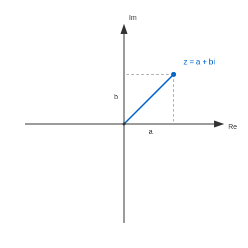

Definition and Properties of Complex Numbers in Complex Numbers and Phasors

Diagram Description: The diagram would illustrate the complex plane, showing the real and imaginary axes with a complex number represented as a point or vector. This visual representation clarifies the spatial relationship between the real and imaginary components of complex numbers.

1.2 The Complex Plane and Visual Representation

The concept of the complex plane is fundamental in understanding complex numbers, especially when applied in physics and electrical engineering. The complex plane, also known as the Argand plane, provides a systematic way to visualize complex numbers, allowing us to interpret their real and imaginary components geometrically.

Each complex number $ z $ can be expressed in the form $ z = a + bi $, where $ a $ is the real part, $ b $ is the imaginary part, and $ i $ is the imaginary unit, defined by $ i^2 = -1 $. Geometrically, we can represent complex numbers as points in the two-dimensional complex plane. The x-axis corresponds to the real part of the number $ a $, while the y-axis corresponds to the imaginary part $ b $. This visualization can greatly simplify many operations and calculations involving complex numbers.

Plotting Complex Numbers

To plot a complex number $ z = a + bi $ on the complex plane:

Locate the point $ a $ on the real axis.
From this point, move vertically $ b $ units along the imaginary axis.
Mark the point where these two movements intersect. This point represents the complex number $ z $.

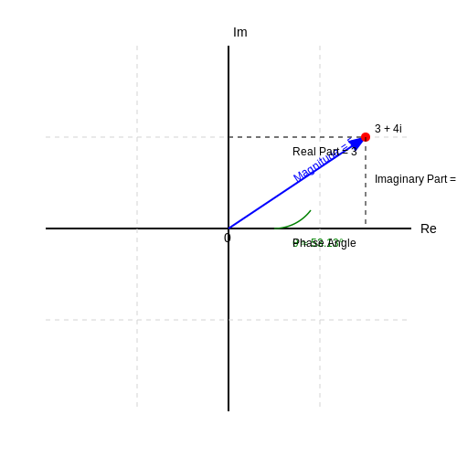
For example, if we have $ z = 3 + 4i $, we would locate the point 3 on the real axis and then move 4 units up along the imaginary axis, concluding at the point (3, 4).

$$ z = a + bi $$

The intersection of the lines at coordinates (3, 4) visually represents the complex number 3 + 4i in the complex plane.

Polarity and Magnitude

The complex plane not only helps us visualize numbers, but it also facilitates calculating and interpreting their properties. For example, we can define the magnitude of a complex number $ z $, also known as its modulus, using the Pythagorean theorem:

$$ |z| = \sqrt{a^2 + b^2} $$

This formula calculates the distance from the origin (0,0) to the point (a,b) on the complex plane. Continuing with our example, the magnitude of $ z = 3 + 4i $ is:

$$ |z| = \sqrt{3^2 + 4^2} = \sqrt{9 + 16} = \sqrt{25} = 5 $$

Understanding the magnitude of a complex number in the context of electrical engineering can be crucial, especially when analyzing alternating current (AC) circuits. The magnitude can represent the peak voltage or current in these contexts.

Phasors in the Complex Plane

Another significant application of the complex plane occurs in representing phasors, which are complex numbers used to represent sinusoidal functions. Specifically, a sinusoidal waveform can be expressed in complex form as:

$$ V(t) = V_m e^{j(\omega t + \phi)} $$

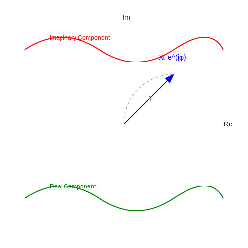
Here, $ V_m $ is the peak voltage, $ \omega $ is the angular frequency, and $ \phi $ is the phase angle. The phasor $ V = V_m e^{j\phi} $ is plotted on the complex plane, with its length representing the magnitude and its angle representing the phase. This approach significantly streamlines calculations involving circuit analysis in the frequency domain, specifically when examining the impedances of resistors, capacitors, and inductors.

The image depicts the phasor representation of an AC voltage source in the complex plane, showcasing both its magnitude and phase angle.

In conclusion, the complex plane is not just a theoretical construct; it provides powerful tools for visualizing and manipulating complex numbers, enhancing our understanding of systems across various engineering and physics applications.

The Complex Plane and Visual Representation in Complex Numbers and Phasors

Diagram Description: The diagram would visually show the complex plane with the x-axis as the real part and the y-axis as the imaginary part, illustrating the placement of complex numbers, including the example of $ z = 3 + 4i $. It will also depict the magnitude of the phasor and its phase angle.

1.3 Arithmetic Operations with Complex Numbers

Complex numbers serve a profound role in various fields of science and engineering, particularly in signal processing, control systems, and electrical engineering. This section explores the arithmetic operations among complex numbers, including addition, subtraction, multiplication, and division, illustrating their implications in practical applications.

Addition and Subtraction of Complex Numbers

Complex numbers are expressed in the form z = a + bi, where a is the real part and b is the imaginary part with i = \sqrt{-1}. The addition and subtraction of complex numbers follows component-wise operations:

For two complex numbers, z_1 = a_1 + b_1 i and z_2 = a_2 + b_2 i, the addition is:

$$ z_1 + z_2 = (a_1 + a_2) + (b_1 + b_2)i $$

The subtraction is:

$$ z_1 - z_2 = (a_1 - a_2) + (b_1 - b_2)i $$

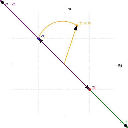
These operations can be visualized in the complex plane, where the x-axis represents the real part and the y-axis the imaginary part. When adding or subtracting, one can think of translating the points in the complex plane.

Multiplication of Complex Numbers

Multiplying complex numbers involves a straightforward application of the distributive property. For our previous examples, let’s consider the multiplication of z_1 and z_2:

$$ z_1 \times z_2 = (a_1 + b_1 i)(a_2 + b_2 i) $$

Applying the distributive property yields:

$$ z_1 \times z_2 = a_1 a_2 + a_1 b_2 i + b_1 a_2 i + b_1 b_2 i^2 $$

Since $ i^2 = -1 $, we simplify the expression:

$$ z_1 \times z_2 = (a_1 a_2 - b_1 b_2) + (a_1 b_2 + b_1 a_2)i $$

Multiplication in the complex plane corresponds to a combination of scaling and rotation, making it essential in the analysis of waves and oscillations.

Division of Complex Numbers

Dividing complex numbers necessitates a technique called "multiplying by the conjugate." The conjugate of a complex number z = a + bi is defined as \overline{z} = a - bi. Suppose we wish to divide z_1 by z_2:

$$ \frac{z_1}{z_2} = \frac{a_1 + b_1 i}{a_2 + b_2 i} \times \frac{a_2 - b_2 i}{a_2 - b_2 i} $$

After simplifying the denominator:

$$ \frac{z_1}{z_2} = \frac{(a_1 a_2 + b_1 b_2) + (b_1 a_2 - a_1 b_2)i}{a_2^2 + b_2^2} $$

Thus, the division results in a new complex number, where the components are expressed as:

$$ \frac{z_1}{z_2} = \left( \frac{a_1 a_2 + b_1 b_2}{a_2^2 + b_2^2} \right) + \left( \frac{b_1 a_2 - a_1 b_2}{a_2^2 + b_2^2} \right)i $$

This operation is particularly useful in analyzing AC circuits, where phasors are predominantly employed. The phasor representation simplifies calculations significantly by transforming differential equations into algebraic ones.

Conclusion

Completing the arithmetic operations on complex numbers enhances understanding of many physical systems, particularly in signal processing and control systems. Each arithmetic operation has geometric and physical interpretations that support a wide range of engineering applications. Mastery of these operations not only solidifies knowledge of complex numbers but also opens doors to advanced applications in technology and research.

Arithmetic Operations with Complex Numbers in Complex Numbers and Phasors

Diagram Description: A diagram would illustrate the components of complex numbers in the complex plane, showing the geometric interpretation of addition, subtraction, and multiplication, highlighting their vector relationships. This visualization would clarify how operations affect the positioning of complex numbers in relation to one another.

2. Definition of Phasors

2.1 Definition of Phasors

In electrical engineering and physics, complex numbers are essential in describing phenomena that vary sinusoidally, such as alternating currents and mechanical vibrations. Within this framework, the concept of phasors emerges as a powerful tool for simplifying the analysis of circuits and systems. A phasor is a complex number that represents a sinusoidal function's amplitude and phase in a compact, manageable form.

A phasor is defined mathematically as:

$$ \mathbf{A} = A_0 e^{j\phi} $$

where A₀ is the amplitude of the sinusoidal signal, j is the imaginary unit (where j² = -1), and φ is the phase angle in radians. In a more practical form, this can also be represented as:

$$ \mathbf{A} = A_0 (\cos(\phi) + j \sin(\phi)) $$

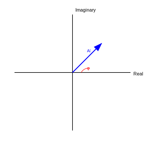
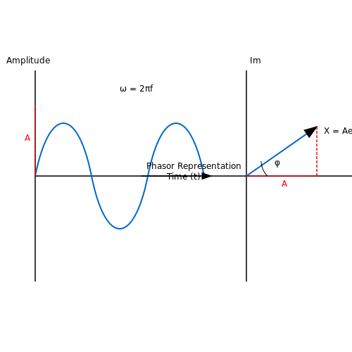
This representation easily connects a sinusoidal function's properties to the rotational dynamics of vectors in a two-dimensional plane. For instance, the amplitude A₀ corresponds to the length of the vector (or radius), while the angle φ describes its rotation about the origin. As the sinusoidal wave oscillates over time, the phasor rotates counterclockwise in this complex plane.

Practical Relevance of Phasors

Phasors simplify computations, particularly in electrical engineering, where analyzing the frequency domain can reveal insights into system behavior. In tasks such as solving circuit equations in alternating current (AC) circuits, phasors allow engineers to switch from differential equations to algebraic equations, thus reducing complexity significantly. In practical applications, phasors are used in:

AC Circuit Analysis: Analyzing the voltages and currents in AC circuits using phasor diagrams enhances understanding of power factors, impedance, and resonance.
Signal Processing: Phasors aid in examining signals, especially in communications, where modulation and demodulation of signals occur.
Control Systems: In control theory, phasors are vital in the design and analysis of systems, especially when assessing stability and response characteristics.

Visualizing Phasors

The geometric representation of phasors can be visualized as rotating vectors in a plane formed by the real and imaginary axes. This visualization reflects how the sinusoidal function 'travels' over time. The radial line's projection on the real axis indicates the instantaneous value of the sinusoidal signal, while its orthogonal component corresponds to the imaginary part—a beautiful illustration of how complex mathematical concepts translate into visual and tangible phenomena.

The utilization of phasors is not confined to technical textbooks; it extends to hands-on simulation and modeling tools that allow both students and professionals to manipulate various parameters and visualize the effects on system behavior. Recognizing the deep-seated interrelation between the mathematical foundation and practical implementations cements phasors as indispensable allies in the engineer's toolkit.

Definition of Phasors in Complex Numbers and Phasors

Diagram Description: The diagram would physically show phasors represented as rotating vectors in a complex plane, with labels indicating amplitude and phase angle. This visual representation would clarify the relationship between phasors and sinusoidal waveforms, bridging the textual explanation with a spatial understanding.

2.2 Relationship Between Sinusoids and Phasors

The analysis of sinusoidal waveforms is a fundamental aspect of electrical engineering and physics, particularly in systems governed by alternating current (AC). To simplify the manipulation and understanding of these sinusoids, we utilize the concept of phasors, an elegant mathematical representation that encapsulates both the amplitude and phase information in a compact form. This subsection will explore how sinusoids relate to phasors, highlighting their benefits and applications in various fields.

Understanding Sinusoids

A sinusoidal function can be expressed mathematically as:

$$ x(t) = A \sin(\omega t + \phi) $$

Here, A represents the amplitude, ω is the angular frequency, t stands for time, and φ is the phase angle. These parameters define the characteristics of the sinusoidal waveform, making it periodic, smooth, and well-understood in both frequency and time domains.

Sinusoids arise in numerous applications, such as sound waves, electrical signals, and vibrations, inherently tying to oscillatory motion. The ability to express these phenomena mathematically allows engineers and physicists to predict behaviors in oscillating systems effectively.

The Phasor Representation

Phasors take advantage of Euler's formula, e^(jθ) = cos(θ) + jsin(θ), to represent sinusoids in the complex domain. The phasor corresponding to the sinusoid can be expressed as:

$$ \mathbf{X} = A e^{j\phi} $$

In this equation, j is the imaginary unit (where j² = -1), and X denotes the phasor representation of the sinusoidal function. The transformation from the time-domain sinusoid to the phasor simplifies the analysis of circuits and systems significantly. It allows engineers to switch from differential equations, which describe time-varying behavior, to algebraic equations that are often easier to solve.

Transitioning from Time Domain to Phasor Domain

The conversion process involves assuming a sinusoidal steady state, where all time variables are encapsulated in their phasor equivalents. For instance, if we have:

$$ v(t) = V_m \sin(\omega t + \phi) $$

the corresponding phasor is simply:

$$ \mathbf{V} = V_m e^{j\phi} $$

This relationship holds true for both voltage and current waveforms in AC circuits, enabling them to be analyzed using techniques such as the superposition principle and impedance analysis.

Applications of Phasors in Electrical Engineering

The utilization of phasors is ubiquitous in the field of electrical engineering. They provide critical insights in:

AC Circuit Analysis: Phasors greatly simplify the calculations of voltages and currents, especially when analyzing circuits with resistors, capacitors, and inductors.
Signal Processing: In telecommunications, phasors assist in the modulation and demodulation of signals, enabling efficient transmission of data.
Control Systems: The design of feedback and control systems often relies on phasor analysis to ensure system stability and performance.

By bridging the understanding of sinusoidal functions and phasors, engineers and physicists can easily maneuver through complex systems, gaining insights that would be cumbersome through time-domain analysis alone.

As we delve deeper into specific applications in subsequent sections, the foundational interplay between sinusoids and phasors will remain central to our explorations.

Relationship Between Sinusoids and Phasors in Complex Numbers and Phasors

Diagram Description: The diagram would show the relationship between sinusoidal waveforms and their phasor representations, illustrating the conversion from time-domain sinusoid to phasor. This visual representation would clarify the transition between the two domains and highlight the key parameters involved.

2.3 Phasor Representation of AC Signals

The significance of phasor representation in alternating current (AC) signal analysis cannot be overstated, especially in the context of complex circuit interactions. This subsection delves into how AC signals, which inherently vary with time, can be efficiently expressed in a phasor format, thus simplifying analysis and facilitating calculations involving sinusoidal waveforms.

Fundamental Concept of Phasors

At its core, a phasor is a complex number that represents the amplitude and phase of a sinusoidal signal. The transition from time-dependent trigonometric functions to an algebraic form can be achieved using Euler's formula, which states that:

$$ e^{j\theta} = \cos(\theta) + j\sin(\theta) $$

Here, $ j $ is the imaginary unit. When an AC signal is expressed in terms of phasors, the sinusoidal form:

$$ x(t) = X_m \cos(\omega t + \phi) $$

can be converted into its phasor representation $ \tilde{X} $ as:

$$ \tilde{X} = X_m e^{j\phi} $$

Expressing AC Signals as Phasors

To illustrate the method of phasor representation, consider an AC voltage signal:

$$ v(t) = V_m \cos(\omega t + \theta) $$

Converting this to phasor form involves noting that $ \tilde{V} = V_m e^{j\theta} $, where $ V_m $ is the peak voltage and $ \theta $ is the phase shift. Execution of this transformational step allows engineers to work with simpler constants instead of time-dependent functions, which is particularly advantageous when analyzing circuits with multiple sinusoidal inputs.

Application in Circuit Analysis

The most profound benefit of phasor representation becomes evident in AC circuit analysis, especially in the context of steady-state sinusoidal circuits. By rewriting Kirchhoff’s laws and Ohm’s law using phasors, one can convert differential equations into algebraic equations. For instance, in an AC circuit comprising resistors, inductors, and capacitors, the impedances are represented as:

Resistance: $ Z_R = R $
Inductance: $ Z_L = j\omega L $
Capacitance: $ Z_C = \frac{1}{j\omega C} $

Where $ R $, $ L $, and $ C $ are the resistance, inductance, and capacitance values, respectively. The analysis of complex circuits through these impedances enables one to readily apply the superposition principle, analyze frequency response, and calculate total power.

Phasor Diagram and Visualization

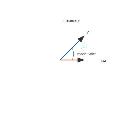
A phasor diagram visually represents the relationship between various voltages and currents in an AC circuit. In this diagram, the length of each phasor corresponds to the amplitude of the voltage or current, while the angle denotes the phase shift. To better understand this concept, consider a phasor diagram depicting a resistive-inductive (RL) circuit:

Conclusion and Practical Implications

The phasor representation of AC signals streamlines both analysis and problem-solving in engineering contexts. It is foundational for understanding complex impedance in AC circuits, facilitating predictions about circuit behavior under sinusoidal excitation. Mastery of this concept not only reinforces theoretical principles but also finds extensive application in fields such as signal processing, telecommunications, and electrical engineering design.

Ultimately, phasors provide a powerful tool for converting complex time-domain problems into manageable frequency-domain representations, embodying a transformative approach for modern engineering analysis.

Phasor Representation of AC Signals in Complex Numbers and Phasors

Diagram Description: The diagram would visually represent the relationship between the voltage and current phasors in an RL circuit, highlighting their amplitudes and phase shift in a clear manner. This visual representation helps illustrate complex vector relationships that are difficult to convey through text alone.

3. Addition and Subtraction of Phasors

3.1 Addition and Subtraction of Phasors

Complex numbers are a powerful tool in electrical engineering, especially when expressed as phasors. These mathematical representations simplify the analysis of sinusoidal signals in both time and frequency domains. In this subsection, we delve into the addition and subtraction of phasors, crucial for various applications, including AC circuit analysis and signal processing.

Understanding Phasor Representation

A phasor is a complex number that represents a sinusoidal function in terms of its magnitude and phase angle. For a sinusoidal waveform described by the equation:

$$ x(t) = A \cos(\omega t + \phi) $$

the phasor corresponding to this waveform is expressed as:

$$ X = A e^{j\phi} $$

where A is the amplitude, j is the imaginary unit, ω is the angular frequency, and φ is the phase angle. The transition to phasor notation allows engineers to employ vector addition methods when dealing with multiple sinusoidal signals.

Vector Representation of Phasors

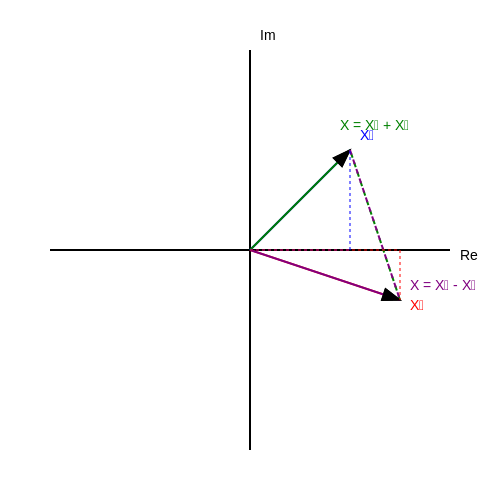
Geometrically, phasors can be represented as vectors in the complex plane, where the horizontal axis corresponds to the real part and the vertical axis corresponds to the imaginary part. To add or subtract phasors, one needs to consider their vector representation. When adding two phasors, say X₁ and X₂, their vector addition is analogous to the triangle rule in vector addition.

Adding Phasors

Consider two phasors expressed in polar form:

$$ X_1 = A_1 e^{j\phi_1} $$ $$ X_2 = A_2 e^{j\phi_2} $$

The sum of these phasors can be represented as:

$$ X = X_1 + X_2 = A_1 e^{j\phi_1} + A_2 e^{j\phi_2} $$

To perform this addition, it is recommended to convert the phasors into their rectangular form:

$$ X_1 = A_1 (\cos(\phi_1) + j \sin(\phi_1) ) $$ $$ X_2 = A_2 (\cos(\phi_2) + j \sin(\phi_2) ) $$

Then, combine the real and imaginary parts:

$$ X = (A_1 \cos(\phi_1) + A_2 \cos(\phi_2)) + j (A_1 \sin(\phi_1) + A_2 \sin(\phi_2)) $$

After computation, the result can be converted back to polar form to express the resultant phasor:

$$ R = |X| = \sqrt{ (A_1 \cos(\phi_1) + A_2 \cos(\phi_2))^2 + (A_1 \sin(\phi_1) + A_2 \sin(\phi_2))^2 } $$ $$ \theta = \tan^{-1}\left(\frac{A_1 \sin(\phi_1) + A_2 \sin(\phi_2)}{A_1 \cos(\phi_1) + A_2 \cos(\phi_2)}\right) $$

Subtracting Phasors

Subtraction follows a similar procedure but involves the negative of the phasor being subtracted. If we want to subtract phasor X₂ from X₁, we treat it as:

$$ X = X_1 - X_2 = A_1 e^{j\phi_1} - A_2 e^{j\phi_2} $$

As with addition, convert to rectangular form, perform the subtraction, and then convert back to polar form. This is invaluable in applications like load analysis, where one must find the net effect of different voltage/current sources.

Practical Relevance in Engineering

The ability to add and subtract phasors is fundamental in electrical engineering, particularly for analyzing alternating current (AC) circuits. Engineers often face multiple voltage and current sources, and phasor addition simplifies calculations significantly. Moreover, understanding these operations allows for designing more efficient systems, whether for power distribution, signal processing, or communication systems.

As we continue exploring complex numbers and phasors, remember the geometric interpretation of these operations can provide insights that purely algebraic methods may obscure.

Addition and Subtraction of Phasors in Complex Numbers and Phasors

Diagram Description: The diagram would illustrate the geometric representation of phasors as vectors in the complex plane, showing how to visually add and subtract these vectors using the triangle rule.

3.2 Multiplication and Division of Phasors

The multiplication and division of phasors are essential operations in the study of alternating current (AC) circuits and signal processing. Understanding these operations allows engineers and physicists to simplify complex problems involving oscillations and waveforms, finding applications in circuit analysis, telecommunications, and control systems.

Multiplying Phasors

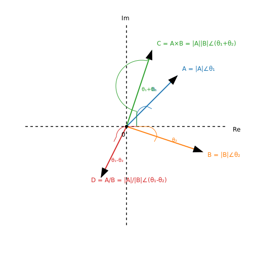
To begin, let's consider two phasors represented by their magnitude and phase: $$ \begin{align*} A & = |A| e^{j\theta_A} \\ B & = |B| e^{j\theta_B} \end{align*} $$ When multiplying two phasors, their magnitudes are multiplied, while their angles (phases) are summed. This can be mathematically represented as: $$ C = AB = |A||B| e^{j(\theta_A + \theta_B)} $$ The geometric interpretation of this operation lies in the unit circle. The magnitude of the resultant phasor $C$ corresponds to the radial distance from the origin to the point represented by the phasor in the complex plane, whereas the angle is determined by the vector sum of the phases of the original phasors. For practical applications, consider two voltages in an AC circuit. Suppose $V_1 = 10 \angle 30^\circ$ V and $V_2 = 5 \angle 60^\circ$ V. Their multiplication can be illustrated as: $$ V = V_1 V_2 = 10 \cdot 5 \angle (30^\circ + 60^\circ) = 50 \angle 90^\circ \text{ V} $$ This means that the combined voltage $V$ has a magnitude of 50 V and a phase of $90^\circ$, indicating that it is purely reactive (an ideal capacitor or inductor).

Dividing Phasors

The division of phasors follows a very similar principle. When one phasor is divided by another, the magnitude of the first is divided by the magnitude of the second and the phase of the first is reduced by the phase of the second: $$ D = \frac{A}{B} = \frac{|A|}{|B|} e^{j(\theta_A - \theta_B)} $$ This operation can again be visualized on the complex plane. The resulting phasor $D$ reflects the relative scale and phase shifts introduced by the division. Taking the previous voltages as an example, if we were to divide $V_1$ by $V_2$: $$ V = \frac{V_1}{V_2} = \frac{10 \angle 30^\circ}{5 \angle 60^\circ} = 2 \angle (30^\circ - 60^\circ) = 2 \angle -30^\circ \text{ V} $$ This indicates that the output voltage $V$ is of magnitude 2 V and leads the reference by $-30^\circ$.

Applications and Practical Relevance

The skills of multiplying and dividing phasors are not only academically vital but also crucial in engineering applications:

Signal Processing: In digital communications, phasor multiplication is used in modulated signals to determine the resultant signal's phase, essential for data recovery.
Power Systems: Understanding how voltages and currents interact in AC circuits aids in the design and analysis of electrical networks, ensuring efficient power distribution.
Control Systems: In feedback loops, the phase relationship between system inputs and outputs is critical for stability, by leveraging phasor operations to simplify calculations.

In summary, mastering the multiplication and division of phasors is crucial for anyone working with AC systems or oscillatory phenomena. The elegant relationship between complex numbers and physical interpretations provides a powerful toolkit for engineers and physicists alike.

Multiplication and Division of Phasors in Complex Numbers and Phasors

Diagram Description: The diagram would visually represent the multiplication and division of phasors on the complex plane, showing how magnitudes and angles interact geometrically. This will help clarify the vector relationships and resulting phasors.

3.3 Impedance and Its Phasor Representation

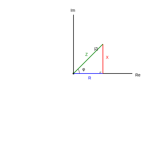
In the analysis of alternating current (AC) circuits, understanding impedance is crucial. Impedance is a complex quantity that extends the concept of resistance to AC circuits. While resistance measures the opposition to current flow in direct current (DC) circuits, impedance incorporates both resistive and reactive components in AC circuits, crucially influencing the behavior of circuit elements when subjected to sinusoidal voltages and currents.

Impedance, denoted by $ Z $, is defined as the ratio of the voltage $ V $ across an element to the current $ I $ flowing through it. It can be expressed mathematically as:

$$ Z = \frac{V}{I} $$

In complex notation, where both voltage and current can be represented as phasors, the impedance can be expressed as:

$$ Z = R + jX $$

Here, $ R $ represents the resistance (in ohms), $ j $ is the imaginary unit, and $ X $ represents the reactance, which can be capacitive ($ X_C $) or inductive ($ X_L $). The reactance is a measure of how much an element resists the change in current due to capacitance or inductance.

Understanding Reactance

To properly grasp impedance, it is essential to understand its components: resistance and reactance. Resistance $ R $ does not depend on frequency, whereas reactance varies with frequency:

Inductive Reactance: This is given by the formula:

$$ X_L = \omega L $$

Capacitive Reactance: Conversely, capacitive reactance is described by:

$$ X_C = \frac{1}{\omega C} $$

In these equations, $ \omega = 2\pi f $ (where $ f $ is the frequency in Hertz), $ L $ is the inductance in henries, and $ C $ is the capacitance in farads. These dependencies highlight the critical role frequency plays in AC circuit behavior.

The Phasor Representation of Impedance

When we analyze circuits in the frequency domain, phasors provide a powerful method to simplify calculations by converting differential equations into algebraic ones. By representing impedances using complex numbers, we enable straightforward computations involving voltage and current.

The phasor representation of impedance simplifies the understanding of how voltage and current relate through their phase angle. The phase angle $ \phi $ between the voltage and the current can be derived from the impedance as follows:

$$ \phi = \tan^{-1}\left(\frac{X}{R}\right) $$

Thus, impedance can also be expressed in polar form:

$$ Z = |Z| e^{j\phi} $$

Where $ |Z| $ is the magnitude of the impedance:

$$ |Z| = \sqrt{R^2 + X^2} $$

Practical Relevance of Impedance and Phasors

In practical applications, engineers often rely on impedance and phasor representations to analyze circuits such as filters, amplifiers, and oscillators. By representing reactive components as phasors, design choices can be easily visualized, optimized, and calculated, particularly in complex network theorems and resonant circuits.

Furthermore, the concept of impedance is foundational in the analysis of transient responses and stability in power systems. Understanding impedance interactions assists engineers in predicting system behaviors when subjected to various loads, ensuring optimal performance and energy efficiency.

In summary, the interplay of resistance and reactance in the context of impedance and its phasor representation provides a robust framework for analyzing and designing AC circuits. This foundational knowledge equips engineers and physicists to navigate the complexities of modern electronic systems with greater confidence and precision.

Impedance and Its Phasor Representation in Complex Numbers and Phasors

Diagram Description: The diagram would show the relationship between impedance, resistance, and reactance in a phasor representation, including the phase angle between voltage and current. It visually represents complex numbers as vectors to elucidate how varying reactance impacts circuit behavior.

4. AC Circuit Analysis Using Phasors

4.1 AC Circuit Analysis Using Phasors

For engineers and physicists working with alternating current (AC) circuits, the application of complex numbers through phasors offers a streamlined approach for analyzing circuit behavior. The fundamental benefit of using phasors arises from their ability to represent sinusoidal functions as rotating vectors in the complex plane. This transformation simplifies mathematical manipulations, making it easier to solve differential equations associated with AC circuits. ### Understanding the Phasor Representation At the heart of the phasor concept is the representation of sinusoidal voltages and currents as complex numbers. Given a sinusoidal function: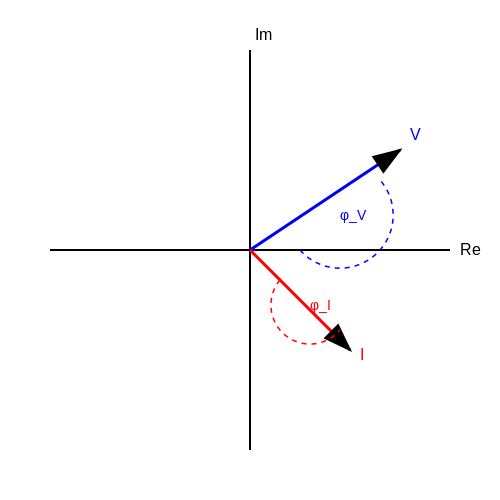

$$ x(t) = X_m \sin(\omega t + \phi) $$

where: - $X_m$ is the amplitude, - $\omega$ is the angular frequency, - $\phi$ is the phase angle. This function can be expressed as a phasor:

$$ X = X_m e^{j\phi} $$

where $j$ is the imaginary unit. In practical terms, the transformation to phasors allows us to work in the frequency domain rather than the time domain, greatly simplifying calculations involving inductors and capacitors. ### Analyzing RLC Circuits with Phasors Let's consider a simple RLC circuit consisting of a resistor (R), an inductor (L), and a capacitor (C) connected in series to an AC voltage source $ V(t) = V_m \sin(\omega t) $. When we apply the phasor representation, we replace all time-varying quantities with their corresponding phasors. The voltage across each element can be expressed as: - Resistor: $ V_R = IR $ - Inductor: $ V_L = j \omega L I $ - Capacitor: $ V_C = \frac{I}{j \omega C} $ Applying Kirchhoff’s voltage law, we obtain the equation:

$$ V = V_R + V_L + V_C $$

Substituting the relationships we established, we find:

$$ V_m e^{j\omega t} = I R + j \omega L I - \frac{I}{j \omega C} $$

Factoring out the current $I$:

$$ V_m e^{j\omega t} = I \left( R + j \omega L - \frac{1}{j \omega C} \right) $$

Let’s denote the total impedance $Z$ of the circuit:

$$ Z = R + j \left( \omega L - \frac{1}{\omega C} \right) $$

The total current $I$ can then be expressed as:

$$ I = \frac{V_m e^{j\omega t}}{Z} $$

### Practical Implications of Phasor Analysis The significance of phasor analysis extends beyond mere mathematical convenience; it allows engineers to predict how circuits will respond to different frequency inputs. Understanding impedance plays a pivotal role in designing circuits for specific applications, including communications, signal processing, and electrical power transmission. Furthermore, these concepts underpin numerous real-world technologies, from the design of filters and amplifiers to the seamless operation of power grids, and they facilitate the integration of renewable energy sources into existing electrical infrastructure. ### Conclusion Phasors offer an invaluable tool for simplifying AC circuit analysis. By converting sinusoidal functions into their complex representations, engineers and physicists can leverage the properties of complex numbers to efficiently analyze and design AC circuits. As technology progresses, the application of phasors in circuit design and analysis continues to be pivotal, particularly in environments increasingly characterized by complex AC signals and varying load conditions.

AC Circuit Analysis Using Phasors in Complex Numbers and Phasors

Diagram Description: The diagram would illustrate the vector representation of phasors in the complex plane, showing the relationship between voltage and current phasors, as well as their respective amplitudes and phase angles. It would visually depict how these phasors rotate with respect to sinusoidal functions, simplifying complex interactions in AC circuit analysis.

4.2 Power Calculations in AC Circuits

Understanding power calculations in AC circuits is vital for engineers and physicists, particularly in designing and analyzing electrical systems. In alternating current (AC) circuits, power is more intricate than in direct current (DC) systems due to the phase shift between voltage and current. This phase difference is represented using complex numbers and phasors, which lend themselves to easier mathematical manipulation.

The Basics of Power in AC Circuits

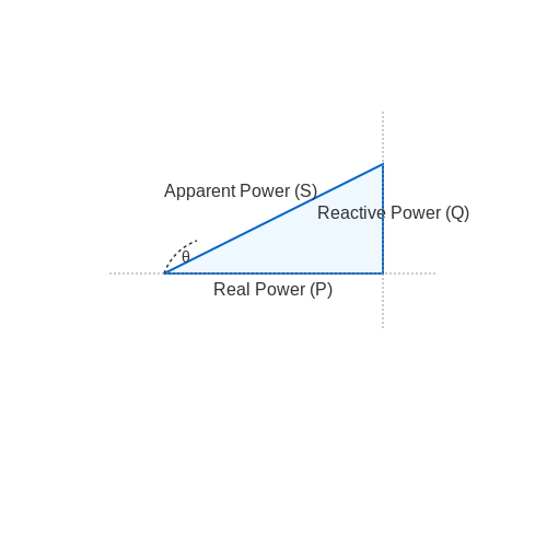
In AC circuits, there are three primary types of power: apparent power (S), real power (P), and reactive power (Q). These are interrelated through the power factor, which is defined as the cosine of the phase angle (θ) between the current and voltage waveforms.

Apparent Power (S): Measured in volt-amperes (VA), it is the product of the root mean square (RMS) voltage and RMS current. It incorporates both real and reactive power.
Real Power (P): Measured in watts (W), it represents the actual power consumed by the circuit to perform work. It is given by the equation:

$$ P = VI \cos(\theta) $$

Reactive Power (Q): Measured in volt-amperes reactive (VAR), it represents the power stored and released by inductors and capacitors, and is given by:

$$ Q = VI \sin(\theta) $$

The relationship between these three types of power can be visualized in the power triangle, where the sides represent real power, reactive power, and apparent power. The hypotenuse corresponds to the apparent power, while the angle θ represents the phase difference between voltage and current. This is crucial in power engineering because it highlights the effects of reactance in AC circuits, which can lead to inefficient energy use.

Complex Power Representation

The concept of complex power (represented as S) combines real and reactive power into a single entity:

$$ S = P + jQ $$

Here, j is the imaginary unit, which is critical in distinguishing real and reactive components. Complex power is measured in volt-amperes (VA) and provides a comprehensive overview of the circuit's power attributes.

Example Calculation

Consider an AC circuit where the RMS voltage is 120 V, and the RMS current is 10 A with a phase angle of 30°. To find real power, reactive power, and apparent power, we can use the following steps:

Calculate apparent power:

$$ S = VI = 120 \times 10 = 1200 \text{ VA} $$

Calculate real power:

$$ P = VI \cos(30^\circ) = 120 \times 10 \times \frac{\sqrt{3}}{2} = 1039.23 \text{ W} $$

Calculate reactive power:

$$ Q = VI \sin(30^\circ) = 120 \times 10 \times \frac{1}{2} = 600 \text{ VAR} $$

This breakdown shows how each component of power plays a significant role in AC circuit analysis, emphasizing the importance of understanding complex numbers and phasors in electrical engineering.

Applications and Implications

Power calculations in AC circuits are not just theoretical; they are critically applied in industry settings such as power generation, distribution, and consumption. Engineers must ensure that power factor corrections are made to minimize energy losses and enhance system efficiency. Moreover, devices like power factor correction capacitors are employed to manage reactive power, improving overall circuit performance. The growing reliance on renewable energy sources also emphasizes the need for precise power calculations to maintain grid stability.

Understanding these concepts will enable professionals to design systems that are not only effective but also efficient, minimizing operational costs and environmental impact.

Power Calculations in AC Circuits in Complex Numbers and Phasors

Diagram Description: The diagram would visually represent the power triangle, illustrating the relationships between real power, reactive power, and apparent power. This visual representation would clearly show how these quantities relate to the phase angle, which is central to understanding power calculations in AC circuits.

4.3 Resonance and Filters in Phasor Domain

In the realm of electrical engineering and physics, understanding resonance and filtering within the phasor domain is crucial for analyzing and designing circuits. This section delves into how resonance phenomena affect circuit behavior and how filters can be ingeniously utilized to select certain frequency components from a signal while rejecting others. The concept of resonance occurs when a system is driven at its natural frequency, leading to increased amplitude of oscillation. In circuits, this typically involves reactive components—inductors and capacitors—that store energy in electric and magnetic fields, respectively. When analyzing such systems in the time domain, the equations can become unwieldy, particularly when dealing with AC signals. However, by transitioning to the phasor domain, a significant simplification can be achieved.

Understanding Resonance in the Phasor Domain

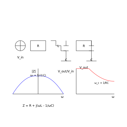
Resonance can be effectively analyzed using the impedance of circuit elements. In an RLC series circuit, we can express the total impedance $ Z $ as follows:

$$ Z = R + j \left( \omega L - \frac{1}{\omega C} \right) $$

where: - $ R $ is the resistance, - $ \omega $ is the angular frequency, - $ L $ is the inductance, - $ C $ is the capacitance, - $ j $ is the imaginary unit. The resonance condition occurs when the reactive components cancel each other out, that is: $$ \omega L = \frac{1}{\omega C} $$ Solving for $ \omega $ gives the resonant frequency:

$$ \omega_0 = \frac{1}{\sqrt{LC}} $$

At this frequency, the impedance is at its minimum, and thus the circuit can draw maximum current. The phenomenon of resonance is particularly vital in applications like radio transmission, where tuning circuits select specific frequencies for desirable signals.

Filters and Their Implementation in the Phasor Domain

Filters are crucial components in signal processing, utilized to manipulate the frequency spectrum of signals. They can be categorized broadly into low-pass, high-pass, band-pass, and band-stop filters. Each of these filters has distinct frequency response characteristics. To illustrate, consider a simple RC low-pass filter. In the phasor domain, the output voltage $ V_{out} $ across the capacitor can be expressed concerning the input voltage $ V_{in} $ as:

$$ V_{out} = \frac{1}{1 + j\frac{\omega RC}{1}} V_{in} $$

The filter's cutoff frequency $ \omega_c $ is determined by:

$$ \omega_c = \frac{1}{RC} $$

Thus, signals with frequencies lower than $ \omega_c $ are allowed to pass, while higher frequencies are attenuated. Visualizing the frequency response plots assists engineers in understanding how the output changes relative to different input frequencies.

Applications of Resonance and Filters

Resonance and filtering techniques play vital roles in numerous practical applications:

Communication Systems: Filters are essential for separating different signal channels in radio and telecommunications.
Audio Systems: Equalizers use filters to boost or cut specific frequency ranges, enhancing audio quality and listener experience.
Power Supply Regulation: Resonance can impact the stability of power electronics, necessitating filtering to reduce noise and ripple.
Measurement Instruments: Using resonant circuits allows for high sensitivity and selectivity in oscillators and sensors.

Recognizing how resonance and filters operate in the phasor domain allows engineers to design secure, efficient, and effective electrical systems. By leveraging phasors, we translate complex time-domain behaviors into manageable algebraic forms, facilitating both analysis and the design of circuits. In conclusion, mastering resonance and filters in the phasor domain enhances the ability to optimize and innovate in various fields, from telecommunications and audio engineering to power electronics. With ongoing advancements in technology, the relevance of these concepts continues to grow, underscoring their importance in both academic study and practical application.

Resonance and Filters in Phasor Domain in Complex Numbers and Phasors

Diagram Description: The diagram would show the relationship between resonance frequency and impedance in an RLC circuit, clearly illustrating how the components interact at resonance. Additionally, a frequency response curve for the RC low-pass filter would visually depict how the output voltage varies with frequency.

5. Complex Frequency and its Significance

5.1 Complex Frequency and its Significance

In the realm of electrical engineering and physics, the behavior of systems in oscillatory and wave-like phenomena can be elegantly described using complex numbers and phasors. One of the profound developments in this subject area is the concept of complex frequency, which extends real frequency to include both amplitude and phase information in a single expression. Understanding complex frequency is pivotal for analyzing systems in the frequency domain, particularly those involving sinusoidal steady-state responses.

Understanding Complex Frequency

In signal processing and communications, the notion of complex frequency arises from the need to represent oscillations comprehensively. The complex frequency $ s $ is defined as: $$ s = \sigma + j\omega $$ where: - $ j $ is the imaginary unit, satisfying $ j^2 = -1 $, - $ \sigma $ is the real part, associated with exponential growth or decay, and - $ \omega $ is the imaginary part, representing angular frequency. In this representation, $ \sigma $ allows for the modeling of transient behaviors—specifically, the growth or decay of signals—while $ \omega $ maintains the cyclic properties intrinsic to oscillations.

Mathematical Properties and Applications

To elucidate these concepts, let’s express a sinusoidal signal in terms of complex frequency. A typical sinusoidal function can be represented as follows: $$ x(t) = A \sin(\omega t + \phi) $$ This can be rewritten using Euler’s formula as: $$ x(t) = \text{Im}(Ae^{j(\omega t + \phi)}) = \text{Im}(Ae^{j\phi}e^{j\omega t}) $$ Substituting the definition of complex frequency, we have: $$ x(t) = \text{Im}(Ae^{j\phi}e^{st}) $$ which demonstrates how sinusoidal waveforms can be analyzed using complex frequency. The significance of this approach becomes evident in system analysis, particularly in transfer function representations. The transfer function $ H(s) $ defines the output to input ratio in the Laplace Transform domain, encapsulating both transient and steady-state behavior of systems. It can be expressed as: $$ H(s) = \frac{Y(s)}{X(s)} $$ where $ Y(s) $ and $ X(s) $ are the Laplace transforms of the output and input signals, respectively.

Practical Relevance

The usage of complex frequency has profound implications in various engineering fields:

Control Systems: Complex frequency allows for the analysis of system stability through pole-zero plots in the s-plane.
Signal Processing: The Fourier Transform utilizes complex frequency to analyze frequency components of signals, allowing for filtering and modulation techniques.
Communications: Modulation schemes like QAM and PSK leverage complex frequency for efficient signal transmission and reception.

By employing complex frequency, engineers can leverage mathematical techniques to derive important insights into the behavior and stability of systems over a continuous range of frequencies.

Conclusion

The introduction of complex frequency has revolutionized the analysis of oscillatory systems, seamlessly integrating amplitude and phase information. Moreover, its applications span numerous domains, emphasizing its critical role in modern engineering practices. As we continue to explore the implications of phasors and complex numbers, it becomes clear that these concepts are indispensable tools in the analytical arsenal of any advanced practitioner in the field. As we move forward, we will further explore the implications of these concepts in real-world applications, demonstrating their utility in solving complex engineering problems.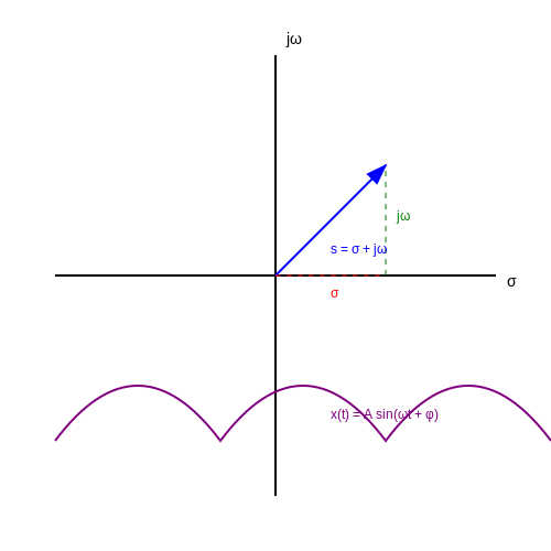

Complex Frequency and its Significance in Complex Numbers and Phasors

Diagram Description: The diagram would illustrate the relationship between complex frequency components, showcasing both the real part ($ \sigma $) and imaginary part ($ j\omega $) on a vector plane, which is essential for understanding their significance in oscillatory behavior.

5.2 The Laplace Transform and its Application in Phasor Analysis

In electrical engineering and control theory, the Laplace Transform serves as a powerful tool to facilitate the analysis of linear time-invariant (LTI) systems. By transforming differential equations into algebraic equations, it allows engineers and physicists to manage system dynamics more effectively. Particularly in phasor analysis, the Laplace Transform helps bridge the gap between time-domain signals and their frequency-domain representations, underscoring its importance in both theoretical and practical applications.

Understanding the Laplace Transform

The Laplace Transform is defined by the integral:

$$ \mathcal{L}\{f(t)\} = F(s) = \int_0^\infty e^{-st} f(t) dt $$

where $ f(t) $ is the original function, $ F(s) $ is the transformed function, $ s $ is a complex frequency variable defined as $ s = \sigma + j\omega $, with $ \sigma $ being the damping factor and $ j $ the imaginary unit. This transformation not only simplifies the mathematics involved but also provides a clearer understanding of system behavior in terms of poles and zeros.

Applications of the Laplace Transform in Phasor Analysis

In phasor analysis, especially in AC circuit analysis, the Laplace Transform proves to be instrumental in analyzing circuits that involve both transient and steady-state responses. An AC signal can be expressed as a combination of its phasor components, which are frequency domain representations of time-domain signals. By employing the Laplace Transform, engineers can analyze circuits with various initial conditions and ascertain system responses over time. An AC voltage source, for example, can be represented in the time domain as:

$$ v(t) = V_m \cos(\omega t + \phi) $$

When we apply the Laplace Transform, we can derive the phasor representation:

$$ V(s) = \frac{V_m e^{j\phi}}{s + j\omega} $$

This transformation reveals the frequency response characteristics of the circuit, allowing one to assess gain margins, phase shifts, and stability.

Solving Differential Equations with Laplace Transforms

A quintessential application of the Laplace Transform lies in solving linear ordinary differential equations (ODEs) that characterize circuit behavior. For instance, consider an RLC circuit described by the second-order differential equation:

$$ L \frac{d^2i(t)}{dt^2} + R \frac{di(t)}{dt} + \frac{1}{C} i(t) = v(t) $$

By taking the Laplace Transform of both sides and applying the initial conditions, we can convert this differential equation into an algebraic form:

$$ L(s^2 I(s) - si(0) - i'(0)) + R(sI(s) - i(0)) + \frac{1}{C} I(s) = V(s) $$

Solving for $ I(s) $ allows us to find the phasor representation of the current in the circuit.

Summary and Real-World Relevance

The transition from the time domain to the Laplace domain and vice versa reveals critical insights into system stability and response characteristics. This offers practical relevance, particularly in control systems and signal processing. The ability to analyze time-invariant systems with variable initial conditions impacts the design of circuit elements in real technologies employed across communications, robotics, and power systems. Through the lens of phasor analysis, the Laplace Transform simplifies complex circuit analysis and supports engineers in optimizing systems for desired performance outcomes. As we continue to see advances in technology, the application of the Laplace Transform and phasors represents a vital intersection of theoretical physics and engineering practice. By mastering these principles, advanced practitioners enhance their capacity to innovate and refine methodologies within the realm of electrical engineering and beyond.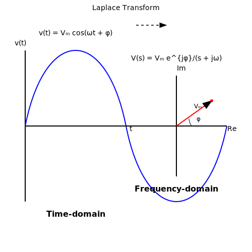

The Laplace Transform and its Application in Phasor Analysis in Complex Numbers and Phasors

Diagram Description: The diagram would visually represent the relationship between time-domain voltage signals and their corresponding phasor representations in the Laplace Transform domain, clarifying the transformation process and system behavior.

5.3 Convolution and Signal Processing Using Phasors

In the realm of electrical engineering and signal processing, phasors play a fundamental role in simplifying the analysis of time-varying signals, especially when tackling linear time-invariant (LTI) systems. This section explores how convolution operates within the context of phasors and its relevance to signal processing.

Understanding Convolution in Signal Processing

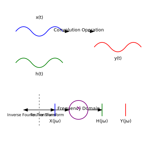
Convolution is a mathematical operation that describes how the shape of one signal impacts another signal. In signal processing, this is particularly vital for determining the output of an LTI system given its input and impulse response. The convolution operation is defined as:

$$ y(t) = (x * h)(t) = \int_{-\infty}^{+\infty} x(τ) h(t - τ) dτ $$

Here, $ x(t) $ represents the input signal, $ h(t) $ the impulse response of the system, and $ y(t) $ the resulting output. The integration accumulates the product of the input signal and a time-shifted version of the impulse response over all time. This integral can become complex, especially in the time domain; however, using phasors significantly simplifies the analysis.

Phasors and Their Role in Convolution

Phasors are complex representations of sinusoidal signals, expressed in the form:

$$ X(j\omega) = \tilde{x}(t) = A e^{j(\omega t + \phi)} $$

where $ A $ is the amplitude, $ \omega $ the angular frequency, and $ \phi $ the phase angle. By transforming the convolution operation into the frequency domain using the Fourier Transform, we can leverage the convolution theorem, which states:

If $ X(j\omega) $ is the Fourier Transform of $ x(t) $, and $ H(j\omega) $ is that of $ h(t) $, then:

$$ Y(j\omega) = X(j\omega) H(j\omega) $$

Thus, convolution in time domain becomes multiplication in frequency domain. The final output $ y(t) $ can be retrieved in its time form by applying the inverse Fourier Transform to $ Y(j\omega) $.

Applications of Convolution in Signal Processing

This transformed and simplified approach greatly enhances the practical applications in various fields, including:

Audio Signal Processing: Here, convolution is used for filtering audio signals or simulating acoustic environments through impulse responses.
Image Processing: Convolution is integral in applying filters, such as blurring or sharpening images, by altering pixel values based on neighboring pixels.
Communications: It aids in designing systems that transmit signals over noisy channels, where the impulse response characterizes the channel behavior.

Understanding the techniques of convolution combined with the elegant representation of signals as phasors allows for a sophisticated approach to signal analysis, offering insights into the behavior of systems in both time and frequency domains.

Summary

Through the exploration of convolution using phasors, we have established a powerful framework that simplifies complex signal interactions in various engineering applications. The next section will delve into the practical implementations and computational techniques of these concepts in modern signal processing tasks.

Convolution and Signal Processing Using Phasors in Complex Numbers and Phasors

Diagram Description: The diagram would illustrate the relationship between input signals, impulse responses, and the resulting output signal during convolution, while also visually depicting how phasors transform this operation from the time domain to the frequency domain.

6. Textbooks and Educational Resources

6.1 Textbooks and Educational Resources

Advanced Engineering Mathematics by K.A. Stroud — This textbook provides an extensive foundation in complex numbers, phasors, and other advanced concepts, complete with exercises, practice problems, and real-world applications.
MIT OpenCourseWare: Linear Algebra — A comprehensive course featuring video lectures that cover complex numbers and their applications in linear algebra, essential for understanding phasors.
Coursera: Electrical Circuits Overview — Offers video lectures and assignments on the basics of electrical circuits, highlighting the role of complex numbers and phasors in circuit analysis.
The Great Courses: Fundamentals of Engineering Calculations — Delivers an engaging guide to engineering calculations, including detailed explanations of complex numbers in practical engineering problems.
Khan Academy: Introduction to Complex Numbers — A series of videos and practice exercises focused on introducing complex numbers, offering fundamental concepts necessary for grasping phasors.
Electrical4U: Phasor Diagrams — Provides detailed explanations about phasor diagrams, illustrating their use in representing alternating current circuits through practical examples.
OpenStax: Precalculus — Free textbook that introduces complex numbers as part of a broader precalculus curriculum, highlighting their utility in various mathematical contexts.

6.2 Online Courses and Lectures

Understanding complex numbers and phasors is crucial for advanced studies in engineering and physics, particularly in areas such as electrical engineering, signal processing, and wave analysis. This subsection provides a selection of highly reputable online resources offering courses and lectures that delve deeply into these topics.

edX Electrical Engineering Courses — Offers a variety of courses on advanced electrical engineering topics, including comprehensive sections on complex numbers and phasor analysis, often taught by leading experts from top universities.
MIT OCW: Signals, Systems, and Inference — Access lectures and materials from MIT's rigorous course which covers the mathematical underpinnings of signals and systems, including detailed exploration of phasors.
Coursera: Linear Circuits - DC Analysis — This course, part of a specialization in circuit design and analysis, includes practical insights into using complex numbers and phasors for analyzing direct current circuits.
YouTube: MIT OpenCourseWare: Signals and Systems — A playlist from MIT's course on signals and systems that covers fundamental theories, including phasor representation and applications in engineering contexts.
Khan Academy: Electrical Engineering — Provides a self-paced learning opportunity with tutorials on complex numbers and their applications in electrical engineering, suitable for brushing up on foundational concepts.
NPTEL: Electrical Engineering - Advanced Courses — India's National Programme on Technology Enhanced Learning offers free access to video lectures focusing on various aspects of electrical engineering, emphasizing complex signal analysis.
MIT OCW: Linear Algebra — For those looking to strengthen their mathematical background, this course offers profound insights into linear algebra concepts, including the manipulation and application of complex numbers.

6.3 Research Papers and Articles

Phasor Studies in Power System Analysis — This research explores the use of phasors in analyzing power systems, focusing on practical implementation of phasor data and their applications in modern electrical grids.
Complex Numbers in Physics and Engineering — The paper discusses the mathematical foundations of complex numbers and their applications across various domains in physics and engineering.
Application of Complex Number Theory in Electromagnetics — It details how complex numbers are utilized in electromagnetic theory to simplify calculations involving wave propagation and signal processing.
Historical Development of Complex Numbers — This article provides a comprehensive historical perspective on the development of complex numbers and their acceptance in scientific computations.
Phasor Measurement and Control Systems — This study examines modern phasor measurement technologies, highlighting their transformative impact on the monitoring and control of power systems.
Complex Variables in Thermodynamics — Explore the innovative use of complex variables within thermodynamics, offering detailed case studies that demonstrate practical applications.
Computational Techniques in Complex Analysis — A thorough analysis of computational strategies used in complex number analysis, providing algorithms and software solutions for engineers.
Phasor Transformations in Structural Mechanics — Discusses the utilization of phasor transformations in simplifying complex mechanical and structural engineering problems.