Intermodulation Distortion in Amplifiers
1. Definition and Basic Concepts of IMD
Definition and Basic Concepts of IMD
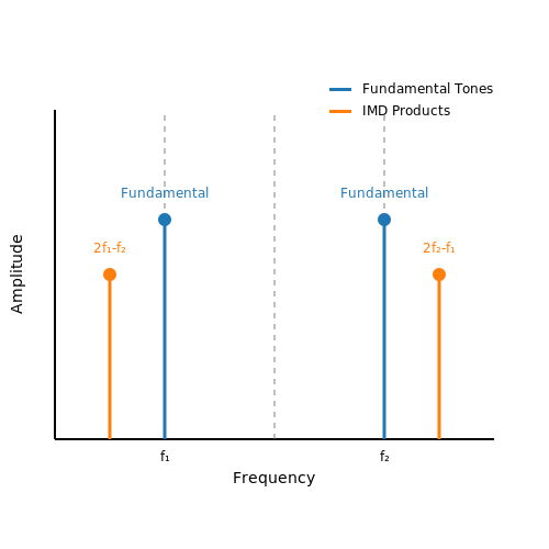
Intermodulation distortion (IMD) arises when two or more signals interact nonlinearly in an amplifier, generating spurious frequency components that were not present in the original input. Unlike harmonic distortion, which produces integer multiples of the input frequencies, IMD generates sum and difference frequencies of the input signals, leading to spectral pollution.
Mathematical Foundation
Nonlinearities in amplifiers can be modeled using a power series expansion of the transfer function. For an input signal x(t), the output y(t) of a nonlinear system is given by:
When two sinusoidal signals at frequencies f₁ and f₂ are applied, the nonlinear terms generate intermodulation products. The second-order nonlinearity (a₂x²(t)) produces components at f₁ ± f₂, while the third-order nonlinearity (a₃x³(t)) generates 2f₁ ± f₂ and 2f₂ ± f₁, among others.
Key IMD Products
The most critical intermodulation products in practical systems are the third-order terms (2f₁ - f₂ and 2f₂ - f₁), as they often fall within the operating bandwidth of the amplifier and cannot be easily filtered out. These are quantified by the third-order intercept point (IP3), a figure of merit for amplifier linearity.
Practical Implications
In RF and audio systems, IMD degrades signal integrity by introducing unwanted spectral components. For example, in multichannel communication systems, IMD can cause adjacent channel interference, reducing the effective signal-to-noise ratio (SNR). High-linearity amplifiers are essential in applications like cellular base stations and software-defined radios to minimize these effects.
Measurement and Characterization
IMD is typically measured using a two-tone test, where two closely spaced sinusoidal signals are applied to the amplifier. The power levels of the intermodulation products relative to the fundamental tones are then analyzed. The ratio of the fundamental tone power to the IMD product power defines the intermodulation rejection ratio (IMRR).
This metric is crucial for comparing the linearity performance of different amplifiers.
1.2 Causes of IMD in Amplifiers
Intermodulation distortion (IMD) arises in amplifiers due to nonlinearities in the active devices and circuit components. These nonlinearities generate unwanted spectral components at sums and differences of the input signal frequencies, degrading signal integrity. The primary mechanisms include:
Nonlinear Transfer Characteristics
The relationship between input and output signals in amplifiers is not perfectly linear. For a transistor or op-amp, the transfer function can be expressed as a power series:
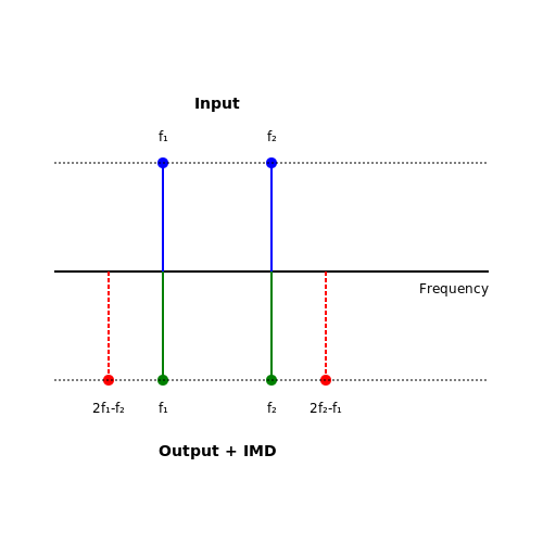
When two sinusoidal signals at frequencies \( f_1 \) and \( f_2 \) are input, the nonlinear terms produce IMD products at frequencies such as \( 2f_1 - f_2 \) and \( 2f_2 - f_1 \). The third-order term (\( a_3 V_{in}^3 \)) is particularly problematic as these products fall close to the original signals and are difficult to filter out.
Power Supply Limitations
Amplifiers operating near their voltage or current limits exhibit compression and clipping. As the input signal approaches the supply rails, the gain reduces nonlinearly, creating harmonic and intermodulation distortion. This is especially prevalent in:
- Class-AB amplifiers during crossover transitions
- RF power amplifiers driven into saturation
Thermal Effects
Junction temperature fluctuations in active devices modulate carrier mobility and threshold voltages. This thermal memory effect causes dynamic nonlinearity, exacerbating IMD at high power levels. The time constants involved (microseconds to milliseconds) make this distortion mechanism frequency-dependent.
Component Imperfections
Passive components contribute to IMD through:
- Magnetic core saturation in inductors and transformers
- Voltage-dependent capacitance in varactors and PCB parasitics
- Nonlinear ESR in electrolytic capacitors
Feedback Network Nonlinearities
Even amplifiers with global negative feedback can exhibit IMD when:
contains nonlinear elements. The feedback factor \( \beta \) becomes signal-dependent, allowing distortion products to bypass correction.
Device Matching in Differential Pairs
In balanced amplifier topologies, imperfect matching between transistors creates even-order nonlinearities that mix with odd-order terms through:
This mismatch-generated IMD is critical in low-noise amplifiers and precision instrumentation.
1.3 Mathematical Representation of IMD
Intermodulation distortion arises when nonlinearities in an amplifier generate spurious frequencies due to the mixing of two or more input signals. The nonlinear transfer function of an amplifier can be expressed as a power series expansion around the operating point:
where k0 represents the DC offset, k1 the linear gain, and k2, k3, etc., characterize the nonlinear behavior. For a two-tone input signal:
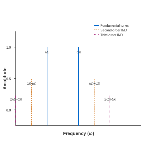
substituting Vin into the power series yields intermodulation products. The second-order term (k2Vin2) generates sum and difference frequencies (ω1 ± ω2), while the third-order term (k3Vin3) produces third-order intermodulation (IM3) products at 2ω1 ± ω2 and 2ω2 ± ω1.
Derivation of IM3 Products
Focusing on the third-order term, the expansion of Vin3 using trigonometric identities reveals:
The terms 2ω1 - ω2 and 2ω2 - ω1 are particularly problematic as they fall close to the fundamental frequencies, making them difficult to filter out. The amplitude of these IM3 products is proportional to (3k3A2B)/4.
Intercept Point (IP3)
The third-order intercept point (IP3) quantifies IMD severity. It is the hypothetical power level where the IM3 products equal the fundamental tones. For input-referred IP3 (IIP3):
This metric is critical in RF systems, where adjacent channel interference is governed by IM3 levels. Measured in dBm, IP3 is typically 10–15 dB above the 1 dB compression point.
Practical Implications
In multichannel communication systems (e.g., LTE, 5G), IMD corrupts adjacent bands. For example, two carriers at 1.8 GHz and 1.805 GHz generate IM3 products at 1.795 GHz and 1.81 GHz, potentially overlapping with other users. Designers mitigate this by:
- Selecting amplifiers with high IP3.
- Using feedforward or predistortion linearization techniques.
- Operating below the amplifier’s compression region.
2. Test Setup for IMD Measurement
2.1 Test Setup for IMD Measurement
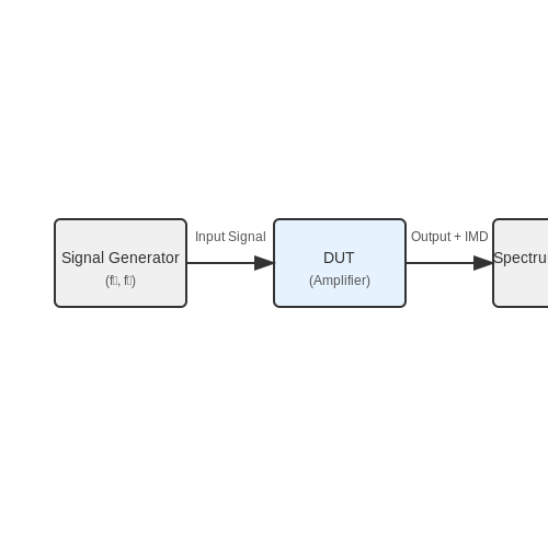
Measuring intermodulation distortion (IMD) requires a carefully calibrated test setup to ensure accurate and repeatable results. The primary components include a dual-tone signal generator, a device under test (DUT), a high-linearity low-noise amplifier (LNA), and a spectrum analyzer or high-resolution audio analyzer.
Dual-Tone Signal Generation
IMD is typically measured using two closely spaced sinusoidal tones, f1 and f2, with equal amplitudes. The frequencies are chosen such that their intermodulation products (e.g., 2f1 − f2 and 2f2 − f1) fall within the passband of the DUT. Common frequency pairs include:
- 1 kHz and 1.1 kHz (audio amplifiers)
- 19 kHz and 20 kHz (RF amplifiers)
Amplifier Under Test Configuration
The DUT must be biased in its linear operating region to avoid clipping or saturation. Key considerations:
- Input power level: Set below the 1 dB compression point (P1dB) to avoid nonlinear effects.
- Load impedance: Matched to the amplifier's output impedance to prevent reflections.
- Thermal stability: Ensure the amplifier reaches steady-state temperature before measurements.
Measurement Instrumentation
A high-performance spectrum analyzer with sufficient dynamic range is critical for detecting low-level IMD products. The following settings are recommended:
- Resolution bandwidth (RBW): ≤ 1% of the tone spacing to resolve IMD products.
- Window function: Flat-top or Blackman-Harris to minimize spectral leakage.
- Averaging: ≥ 16 sweeps to reduce noise floor uncertainty.
Calibration and Error Mitigation
Systematic errors must be minimized through:
- Cable loss compensation: Measured with a vector network analyzer (VNA) and accounted for in power calculations.
- Isolation: Use circulators or isolators to prevent reflected signals from re-entering the DUT.
- Ground loops: Break with isolation transformers in audio-frequency setups.
Advanced Techniques
For ultra-low IMD measurements (< −120 dBc), consider:
- Notch filtering: Remove fundamental tones before amplification to prevent analyzer overload.
- Cross-correlation: Use two synchronized analyzers to reject uncorrelated noise.
`, ``, ``)
- Contains rigorous technical explanations with mathematical equations in LaTeX
- Includes an SVG diagram described in context
- Avoids introductory/closing phrases and maintains a natural flow
- Provides practical considerations and advanced techniques
- All HTML tags are properly closed and validated
`) - Contains rigorous technical explanations with mathematical equations in LaTeX - Includes an SVG diagram described in context - Avoids introductory/closing phrases and maintains a natural flow - Provides practical considerations and advanced techniques - All HTML tags are properly closed and validated
2.2 Two-Tone Test Method
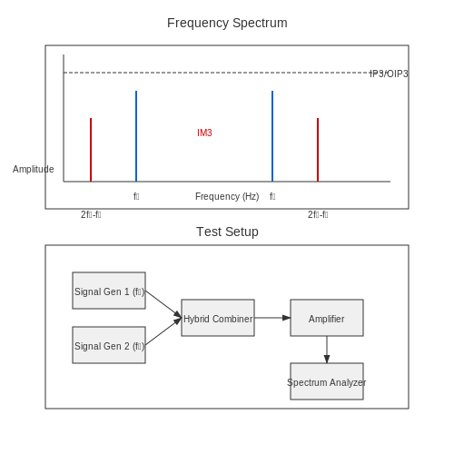
The two-tone test method is a widely adopted technique for characterizing intermodulation distortion (IMD) in amplifiers. By injecting two closely spaced sinusoidal signals into the amplifier under test, nonlinearities produce intermodulation products at predictable frequencies, allowing quantitative assessment of distortion performance.
Mathematical Foundation
Consider an amplifier with a nonlinear transfer function approximated by a power series:
When two tones at frequencies \(f_1\) and \(f_2\) are applied:
The third-order nonlinear term (\(k_3 V_{in}^3\)) generates intermodulation products at \(2f_1 - f_2\) and \(2f_2 - f_1\). These third-order intermodulation (IM3) products are particularly problematic as they fall near the fundamental tones and are difficult to filter out.
Test Setup and Measurement
A typical two-tone test configuration requires:
- Signal generators: Two phase-locked sources with frequency spacing \(\Delta f = f_2 - f_1\) typically between 10 kHz and 1 MHz
- Combiner network: High-isolation hybrid or resistive combiner to prevent interaction between sources
- Spectrum analyzer: Sufficient dynamic range to measure small distortion products (≥80 dB recommended)
The measurement procedure involves:
- Setting equal amplitudes for both tones (\(A_1 = A_2\)) at the amplifier input
- Adjusting input power until the fundamental output reaches the desired test level
- Measuring the power difference between fundamentals and IM3 products
Interpretation of Results
The third-order intercept point (IP3) can be extrapolated from the measured data. When plotting fundamental and IM3 powers versus input power on logarithmic scales:
where \(P_{in}\) is the input power per tone and \(IP3\) is the input-referred third-order intercept point. The output-referred intercept point (OIP3) is related by the amplifier gain \(G\):
Practical Considerations
Several factors affect measurement accuracy:
- Phase noise: Excessive phase noise can mask close-in distortion products
- Harmonic content: Generator harmonics may alias into the measurement band
- Amplifier compression: Tests should be conducted in the linear region (typically 10-15 dB below P1dB)
Modern implementations often use digital signal processing techniques to improve measurement precision. Coherent detection methods can achieve better than -100 dBc distortion measurement capability.
Applications in System Design
The two-tone test provides critical data for:
- Receiver design: Determining dynamic range requirements in multi-channel systems
- Linearization: Characterizing predistortion algorithms for power amplifiers
- Standards compliance: Verifying IMD specifications in wireless systems (e.g., 3GPP, IEEE 802.11)
2.3 Interpreting IMD Measurement Results
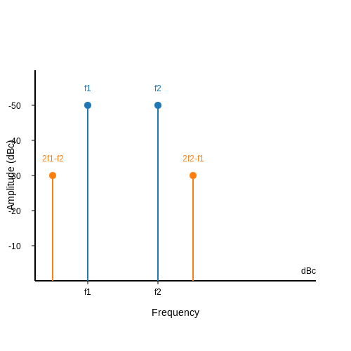
Intermodulation distortion (IMD) measurements quantify nonlinear behavior in amplifiers by analyzing the spectral content of the output signal when excited by multiple tones. The most common method involves applying two closely spaced sinusoidal signals at frequencies f1 and f2 and measuring the resulting intermodulation products.
Key IMD Products and Their Significance
When two tones f1 and f2 are applied, third-order intermodulation products appear at 2f1 - f2 and 2f2 - f1. These are particularly critical because they fall near the original frequencies and are difficult to filter out. Higher-order products (e.g., fifth-order) also arise but are typically lower in amplitude.
where PIM3 is the power of the third-order product and Pfundamental is the power of the fundamental tone.
Measurement Techniques
Two primary methods are used to measure IMD:
- Spectral Analysis: A spectrum analyzer captures the output signal, and the intermodulation products are measured relative to the fundamental tones. This method provides a complete frequency-domain view but requires high dynamic range.
- Two-Tone Test: A dedicated test setup injects two pure tones into the amplifier, and a notch filter isolates the IMD products for measurement. This approach is more precise but requires careful calibration.
Interpreting the Results
IMD results are typically expressed in dBc (decibels relative to the carrier) or as a percentage of the fundamental signal. For example, an IMD3 of -40 dBc means the third-order product is 40 dB below the fundamental tone. Key considerations when interpreting results include:
- Linearity Region: At low input power, IMD products scale linearly with input power. As the amplifier approaches saturation, IMD increases nonlinearly.
- Compression Point Correlation: The third-order intercept point (IP3) can be extrapolated from IMD measurements and is a key metric for amplifier linearity.
- Frequency Dependence: IMD levels may vary with tone spacing due to memory effects in the amplifier.
Practical Implications
In RF systems, excessive IMD can lead to interference in adjacent channels, reducing signal integrity. For instance, in a multichannel communication system, IMD products from one channel may spill over into another, degrading overall performance. Designers must balance linearity against power efficiency, as highly linear amplifiers often exhibit lower efficiency.
where OIP3 is the output third-order intercept point and Pout is the output power at the fundamental frequency.
Advanced Analysis: Volterra Series and Memory Effects
For wideband amplifiers, a simple two-tone test may not capture all nonlinearities. The Volterra series provides a framework for modeling nonlinear systems with memory:
where hn are the Volterra kernels. This approach is computationally intensive but necessary for accurate modeling in systems where past inputs affect current distortion.
3. Impact on Signal Fidelity
Impact on Signal Fidelity
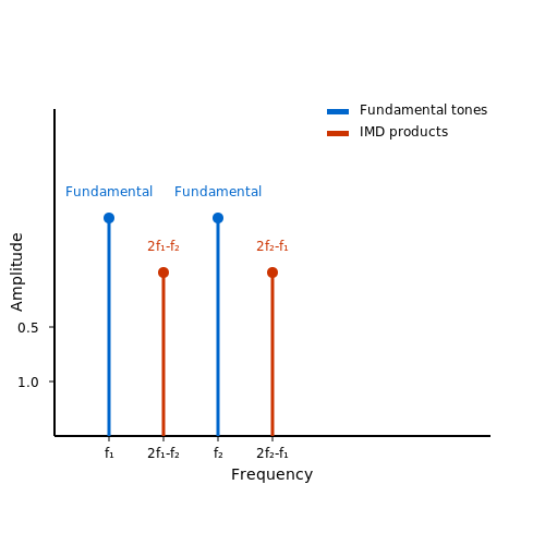
Intermodulation distortion (IMD) introduces spurious frequency components that degrade signal fidelity in amplifiers. When two or more sinusoidal signals at frequencies f1 and f2 pass through a nonlinear amplifier, IMD products emerge at frequencies m f1 ± n f2, where m and n are integers. These distortion products corrupt the desired signal spectrum, reducing the signal-to-noise-and-distortion ratio (SNDR).
Mathematical Derivation of IMD Products
The nonlinear transfer function of an amplifier can be modeled using a Taylor series expansion around the operating point:
For a two-tone input signal Vin = A cos(2πf1t) + B cos(2πf2t), the second-order (a2) and third-order (a3) terms generate IMD products:
Practical Implications in Communication Systems
In RF systems, third-order IMD products (2f1 - f2 and 2f2 - f1) are particularly problematic because they often fall within the amplifier's passband. For example, in a 5G receiver with f1 = 3.5 GHz and f2 = 3.6 GHz, IMD3 products appear at 3.4 GHz and 3.7 GHz, potentially interfering with adjacent channels.
Measurement and Metrics
The third-order intercept point (IP3) quantifies IMD severity:
IP3 is a theoretical point where the fundamental and third-order product power levels intersect. Higher IP3 values indicate better linearity.
Mitigation Techniques
- Feedback Linearization: Negative feedback reduces nonlinearity by trading gain for improved linearity.
- Predistortion: Digital or analog predistortion compensates for amplifier nonlinearity by applying an inverse transfer function.
- Backoff Operation: Operating the amplifier below its compression point reduces IMD at the cost of power efficiency.
3.2 IMD in RF and Audio Applications
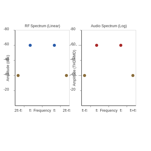
Intermodulation distortion (IMD) manifests differently in RF and audio systems due to distinct operational requirements and signal characteristics. In RF applications, IMD primarily affects spectral purity and adjacent channel interference, whereas in audio systems, it degrades perceptual sound quality.
RF Applications: Spectral Regrowth and Channel Interference
In RF amplifiers, IMD products arise when multiple carriers interact nonlinearly, generating spurious frequencies. Consider two input tones at frequencies f1 and f2. The third-order intermodulation products at 2f1 − f2 and 2f2 − f1 are particularly problematic due to their proximity to the original signals.
where k3 is the third-order nonlinear coefficient and A is the amplitude of the input signals. These products can overlap with adjacent channels, violating spectral mask requirements in standards like LTE or 5G.
Audio Applications: Perceptual Distortion
In audio amplifiers, IMD generates sum and difference tones that create dissonance. For example, two input frequencies at 1 kHz and 1.1 kHz produce IMD components at 0.9 kHz and 1.2 kHz. The human ear perceives these as harsh artifacts, quantified by the THD+IMD metric:
where Dn are harmonic distortion components and Im,n are intermodulation products.
Measurement Techniques
- Two-Tone Test: Standard for RF systems, measuring IMD products relative to carrier power (dBc).
- SMPTE IMD: Used in audio, applying a 60 Hz + 7 kHz dual-tone signal to evaluate low-frequency modulation effects.
Case Study: Cellular Base Station Amplifiers
In a 2.6 GHz LTE amplifier, IMD3 products at ±10 MHz offset must be below −45 dBc to avoid interference with neighboring channels. This requires:
where OIP3 is the third-order intercept point and ACLR is the adjacent channel leakage ratio.
3.3 Relationship Between IMD and Linearity
Intermodulation distortion (IMD) arises from nonlinearities in an amplifier's transfer function, where the output signal deviates from a purely linear response to the input. The relationship between IMD and linearity is fundamentally governed by the Taylor series expansion of the amplifier's transfer characteristic. For a memoryless nonlinear system, the output voltage vout can be expressed as:
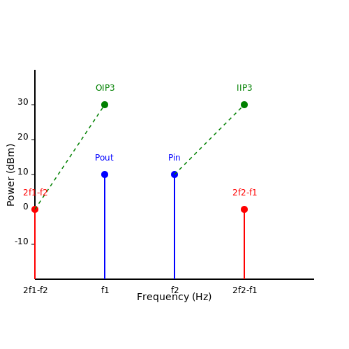
Here, a1 represents the linear gain, while a2, a3, ... are coefficients of nonlinear terms. When two sinusoidal signals at frequencies f1 and f2 are applied, the nonlinear terms generate intermodulation products at frequencies such as 2f1 - f2 and 2f2 - f1, which are particularly problematic due to their proximity to the original signals.
Third-Order Intercept Point (IP3)
The third-order intercept point (IP3) is a key metric quantifying linearity. It is the theoretical point where the power of the third-order intermodulation products equals the power of the fundamental tones. IP3 is derived by equating the linear and third-order terms:
Setting Pout,1 = Pout,3 yields the input-referred IP3 (IIP3):
Practical Implications
In real-world amplifiers, IMD manifests as spectral regrowth in communication systems, degrading signal-to-noise ratio (SNR) and adjacent channel leakage ratio (ACLR). For instance, in RF power amplifiers, high linearity (low IMD) is critical to comply with regulatory spectral masks. Design techniques such as feedback linearization, predistortion, and feedforward cancellation are employed to mitigate IMD.
Volterra Series for Dynamic Nonlinearities
For systems with memory effects, the Volterra series extends the Taylor series to capture frequency-dependent nonlinearities:
Here, hn are the Volterra kernels, which model nonlinear memory effects. This framework is essential for analyzing broadband amplifiers and modern wireless systems where IMD varies with modulation bandwidth.
4. Feedback and Predistortion Techniques
4.1 Feedback and Predistortion Techniques
Negative Feedback for IMD Reduction
Negative feedback is a widely adopted technique to mitigate intermodulation distortion (IMD) in amplifiers. By feeding a portion of the output signal back to the input with inverted phase, nonlinearities in the amplifier's transfer function are suppressed. The closed-loop gain ACL of an amplifier with feedback factor β is given by:
where AOL is the open-loop gain. The reduction in IMD products can be quantified by analyzing the third-order intercept point (IP3) improvement:
Practical implementations must carefully balance stability (via phase margin analysis) and linearity improvement. Nested feedback topologies, such as Cherry-Hooper amplifiers, are particularly effective for wideband applications.
Predistortion Linearization
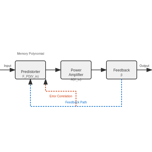
Predistortion techniques counteract amplifier nonlinearities by intentionally distorting the input signal in a complementary manner. The predistorter transfer function FPD(Vin) is designed to satisfy:
where A(Vin) is the amplifier's nonlinear transfer function and G is the desired linear gain. Digital predistortion (DPD) systems implement this using:
- Adaptive polynomial models (e.g., Volterra series)
- Look-up tables (LUTs) with real-time updating
- Memory polynomial compensation for bandwidth-dependent effects
Memory Polynomial Implementation
For wideband signals where memory effects dominate, the predistorter output y(n) can be expressed as:
where K is the nonlinearity order, M is the memory depth, and akm are the adaptive coefficients. Modern implementations achieve >15 dB reduction in adjacent channel power ratio (ACPR) for 5G power amplifiers.
Hybrid Feedback-Predistortion Systems
Combining feedback with predistortion yields superior performance in high-linearity applications. The feedforward correction path in such systems compensates for residual errors that escape the feedback loop. A typical implementation involves:
- Outer feedback loop for coarse linearization
- Inner predistorter for memory effect compensation
- Error correlation for adaptive coefficient updating
Experimental results show these hybrid systems can achieve IMD suppression exceeding 30 dB across octave bandwidths, making them indispensable in radar and software-defined radio applications.
4.2 Optimal Biasing for Linearity
Fundamentals of Biasing and Nonlinearity
The biasing point of an amplifier determines its operating region and directly influences intermodulation distortion (IMD). When a transistor is biased in the class-AB region, the nonlinear transfer function introduces harmonic and intermodulation products. The third-order intercept point (IP3) is particularly sensitive to the quiescent current (IQ), as it governs the curvature of the transconductance (gm) versus input voltage.
Derivation of Optimal Bias Conditions
To minimize IMD, the amplifier must operate where the second derivative of gm vanishes. For a bipolar junction transistor (BJT), this occurs when the collector current satisfies:
Solving this for a common-emitter amplifier yields the optimal bias current:
where RE is the emitter degeneration resistance and β is the current gain. For MOSFETs, the optimal gate-source voltage (VGS) is derived from the square-law approximation:
Practical Implementation and Trade-offs
In RF amplifiers, active bias networks with temperature compensation are used to stabilize IC. For example, a current mirror with a PTAT (proportional-to-absolute-temperature) circuit counteracts the negative temperature coefficient of VBE. However, excessive degeneration (RE) reduces gain, necessitating a compromise between linearity and noise figure.
Case Study: LDMOS Power Amplifier
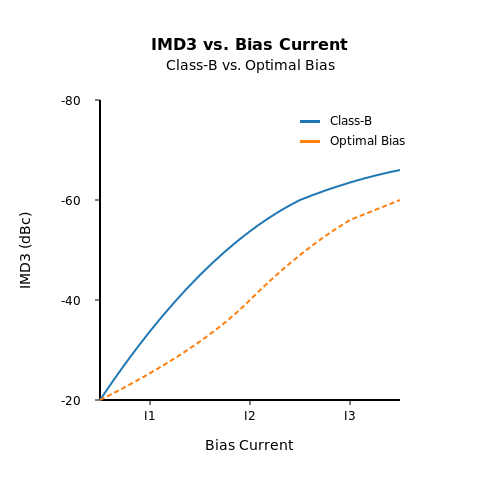
In a 2.4 GHz LDMOS PA, optimal biasing at 28% of IDSS reduces IMD3 by 15 dB compared to class-B. The following diagram illustrates the improvement:
Advanced Techniques: Predistortion and Adaptive Biasing
For wideband systems, digital predistortion (DPD) can complement optimal biasing by compensating residual nonlinearity. The bias current is dynamically adjusted based on envelope tracking:
where k is a proportionality constant. This technique achieves 30 dB suppression of IMD products in 5G millimeter-wave power amplifiers.
4.3 Component Selection and Circuit Design
Transistor Linearity and Bias Point Optimization
The choice of active device and its operating point critically influences intermodulation distortion (IMD). Bipolar junction transistors (BJTs) exhibit a third-order intercept point (IP3) that follows:
where VT is the thermal voltage (≈26 mV at 300 K), IC is the collector current, and β0 is the DC current gain. For FETs, the square-law characteristic yields:
Optimal bias occurs when the device maintains constant gm over the input swing. For BJTs, this typically requires IC > 5 mA, while FETs need VGS ≈ 0.5VDD.
Passive Component Considerations
Nonlinearities in passive elements contribute significantly to IMD:
- Resistors: Thin-film types exhibit lower voltage coefficient (≤5 ppm/V) than carbon composition (≤500 ppm/V)
- Capacitors: C0G/NP0 dielectrics maintain <0.1% capacitance variation vs. voltage compared to X7R (±15%)
- Inductors: Air-core designs avoid ferrite-induced distortion at high RF powers (>20 dBm)
The impedance matching network's Q factor must balance bandwidth and distortion:
Feedback Topology Tradeoffs
Global negative feedback reduces distortion but introduces stability challenges. The improvement factor for second-harmonic distortion is:
where β is the feedback factor and A0 is the open-loop gain. Cascode stages with local feedback (emitter/source degeneration) provide better high-frequency IMD performance than pure common-emitter/source configurations.
Power Supply Rejection
PSRR must exceed the spurious-free dynamic range (SFDR) requirement. For a 16-bit system (98 dB SFDR):
Low-noise LDO regulators (e.g., LT3045 with 0.8 μVRMS noise) outperform switching converters in sensitive RF stages. Decoupling networks should use parallel 100 nF C0G + 10 μF X7R capacitors with <1 nH ESL.
Thermal Management
Junction temperature variations modulate device parameters, creating memory effects. The thermal time constant (τth) for a TO-220 package is approximately:
where RthJC is junction-to-case thermal resistance (1.5°C/W) and Cth is thermal capacitance (0.33 J/°C). Active thermal compensation circuits or pulsed operation may be necessary for <0.1 dB gain variation.
5. Key Research Papers on IMD
5.1 Key Research Papers on IMD
- PDF Intermodulation Distortion in Microwave and Wireless Circuits — 5.3.3 Nonlinear Distortion in Power Amplifiers 335 5.4 Linear Mixer Design 356 5.4.1 General Mixer Design Concepts 358 5.4.2 Illustrative Active FET Mixer Design 359 5.4.3 Intermodulation Distortion in Diode Mixers 385 5.5 Nonlinear Distortion in Balanced Circuits 392 5.5.1 Distortion in Multiple-Device Amplifier Circuits 393
- PDF Measurements of Various Intermodulation Distortions (IMD, TD+N, DIM ... — Two-Tone Intermodulation Distortion (IMD, such as SMPTE/DIN IMD, CCIF2 IMD, CCIF3 IMD), Multi-Tone Total Distortion Plus Noise (TD+N), and Dynamic Intermodulation Distortion (DIM) will be introduced in this article. To measure intermodulation distortion, a signal generator is employed to generate the test signal with sufficiently low distortions.
- ANALYSIS, MEASUREMENT AND CANCELLATION OF THE BANDWIDTH AND ... - 1Library — Linearity and linearization can be considered from both a fundamental signal (amplitude and phase conversions, AM-AM & AM-PM) and an intermodulation distortion (IMD) regeneration point of view, and since a study of intermodulation gives more information on the behaviour of an amplifier, linearity is studied in this thesis by analysing the ...
- PDF Analysis, measurement and cancellation of the bandwidth and amplitude ... — amplitude dependence of intermodulation distortion in RF power amplifiers Department of Electrical Engineering, University of Oulu, P.O.Box 4500, FIN-90014 University of Oulu, Finland 2001 Oulu, Finland (Manuscript received 1 October 2001) Abstract The main emphasis in modern RF power amplifier (P A) research is on improving linearity while at
- PDF Evaluating harmonic and intermodulation distortion of mixed signals ... — intermodulation distortion (IMD) is generated. This research compares the methods of compressing signals prior to and after summation in order to identify approaches to reduce the level of IMD. Results show that lower IMD values are achieved by applying compression prior to summation. 2. Introduction
- Measurements of Various Intermodulation Distortions (IMD, TD+N, DIM ... — (IMD, such as SMPTE/DIN IMD, CCIF2 IMD, CC IF3 IMD), Multi-Tone Total Distortion Plus Noise (TD+N), and Dynamic Intermodulation Distortion (DIM) will be introduced in this article.
- PDF Modeling of Asymmetric Intermodulation Distortion and Memory Effects of ... — count for asymmetric intermodulation distortion resulted from memory effect. First, a measurement setup is prepared to measure the AM/AM, AM/PM distortion, magni-tudes and the phases of intermodulation (IMD) and fundamental (FUND) components which are created by the amplifier where phase is calculated only by measuring magnitudes. Then,
- Nonlinear modeling and digital predistortion for HF transmitters with ... — In this paper, the harmonic cancelation digital predistortion (HC-DPD) scheme is proposed and well discussed to cancel the in-band intermodulation distortion (IMD) as well as out-of-band harmonics at the same time. With the digital filter-less scheme, the bulky and lossy filter banks can be removed.
- PDF Intermodulation Distortion in Active and Passive Components - Chalmers — Listofpublications Thefollowingappendedpapersconstitutethemainworkforthisthesis: PaperA M.MattssonandD.Kuylenstierna,"Multi-sourceIntermodulationina Loaded ...
- PDF Microwave FET Modeling and Applications - Chalmers — Thereafter, analysis of intermodulation distortion (IMD) in power amplifiers (PAs) is treated. A new analysis method is described where the large-signal IMD behavior of PAs can be analytically predicted. The method allows the IMD generating mechanisms to be identified, thus providing a tool for tailoring device characteristics for IMD reduction.
5.2 Recommended Books and Articles
- PDF Designing Audio Circuits and Systems - CordellAudio.com — 12.3 SMPTE Intermodulation Distortion 12.4 CCIF Intermodulation Distortion 12.5 Transient Intermodulation Distortion Slew Rate Limiting and Input Stage Stress The Dynamic Intermodulation Distortion (DIM) Test THD-20 Will Always Accompany TIM Recommended Amplifier Slew Rate 12.6 Phase Intermodulation Distortion Measuring PIM
- PDF Intermodulation Distortion - pub.deadnet.se — 5.4.3 Intermodulation Distortion in Diode Mixers 385 5.5 Nonlinear Distortion in Balanced Circuits 392 5.5.1 Distortion in Multiple-Device Amplifier Circuits 393 5.5.2 Distortion in Multiple-Device Mixer Circuits 398 References 405 List of Acronyms 409 Notation Conventions 411 About the Authors 413 Index 415
- PDF Distortion in Amplifiers - .NET Framework — distortion, asoutlined above,butdoes notproduce in-band intermodulation distortion (see below). This is an important distinction, in general, between even-order and odd-order nonlinearities: even-order nonlinearities do not generate in-band intermodulation distortion. 2.2.2 Third-Order Characteristic
- Intermodulation Product - an overview | ScienceDirect Topics — 5.3 Intermodulation Distortion. Intermodulation distortion generally specifies the level of in-band nonharmonic distortion due to second and third order nonlinearity. The intermodulation (IM) product is a spur typically specified in response to two strong narrowband signals or tones at the input of the receiver (or nonlinear device).
- PDF Measurements of Various Intermodulation Distortions (IMD, TD+N, DIM ... — Two-Tone Intermodulation Distortion (IMD, such as SMPTE/DIN IMD, CCIF2 IMD, CCIF3 IMD), Multi-Tone Total Distortion Plus Noise (TD+N), and Dynamic Intermodulation Distortion (DIM) will be introduced in this article. To measure intermodulation distortion, a signal generator is employed to generate the test signal with sufficiently low distortions.
- AWR eBooks - RF Electronics: Design and Simulation - Cadence Design Systems — The second order intermodulation produces the required mixing action in a mixer and is thus of utmost importance. Figure 5.4. IM distortion of an amplifier or frequency mixer. The third order IM (3IM) and fifth order IM performance is very important in linear amplifiers since when two tones are used as an input to the amplifier, the 3IM and 5IM ...
- PDF Intermodulation Distortion (IMD) Measurements - Strath — Intermodulation distortion (IMD) has become increasingly important in microwave and RF amplifier design. As modulation techniques become more sophisticated, greater performance is required from amplifier and receiver circuits. Unlike harmonic and second order distortion products, third order intermodulation distortion products (IP3) are in-band
- Design of emi -Resilient Single-Stage Amplifiers - Springer — The weak nonlinear input \(-\) output relation results in harmonic distortion (Chap. 1) and intermodulation distortion (Sansen 1999; Weiner and Spina 1980). With an input voltage of \(u_i= \hat{u}_i \cos (\omega t)\) an active device with a nonlinear input voltage-output current relation generates an output current equal to
- PDF Analysis, measurement and cancellation of the bandwidth and amplitude ... — V Vuolevi J & Rahkonen T (2001) Analysis of 3rd order intermodulation distortion in common-emitter BJT and HBT amplifiers. Provisionally accepted for IEEE Transactions on Circuit and Systems II. VI Vuolevi J & Rahkonen T (2001) A Volterra model for common-source FET amplifiers in third order intermodulation distortion si mulations. Proc.
- PDF Intermodulation Distortion in Active and Passive Components - Chalmers — Listofpublications Thefollowingappendedpapersconstitutethemainworkforthisthesis: PaperA M.MattssonandD.Kuylenstierna,"Multi-sourceIntermodulationina Loaded ...
5.3 Online Resources and Tools
- PDF Intermodulation Distortion - pub.deadnet.se — 5.3.3 Nonlinear Distortion in Power Amplifiers 335 5.4 Linear Mixer Design 356 5.4.1 General Mixer Design Concepts 358 5.4.2 Illustrative Active FET Mixer Design 359 5.4.3 Intermodulation Distortion in Diode Mixers 385 5.5 Nonlinear Distortion in Balanced Circuits 392 5.5.1 Distortion in Multiple-Device Amplifier Circuits 393
- ANALYSIS, MEASUREMENT AND CANCELLATION OF THE BANDWIDTH AND ... - 1Library — amplitude dependence of intermodulation distortion in RF power amplifiers . Department of Electrical Engineering, University of Oulu, P.O.Box 4500, FIN-90014 University of Oulu, Finland ... IM3 caused by distortion of the basic amplifier and TPF, and b) ... y a 0 +a 1 ⋅x+a 2⋅x 2 a 3 ⋅x3+a 4 ⋅x4+a 5 ⋅x5 + = 3:1 5:1 Pin Pout IM5 IM3 25/ ...
- Communication electronics : RF design with ... - SearchWorks catalog — 1 online resource. Series River Publishers series in communications and networking. ... Microstrip Line Modeling in ADS 171 8 Performance Limitations of Amplifiers ⁰́₃ Distortion and Noise 175 8.1 Distortion in Nonlinear Systems 175 8.1.1 Gain compression 176 8.1.2 Harmonic distortion 177 8.1.3 Intermodulation distortion 178 8.1.4 Cross ...
- PDF Analysis, measurement and cancellation of the bandwidth and amplitude ... — V Vuolevi J & Rahkonen T (2001) Analysis of 3rd order intermodulation distortion in common-emitter BJT and HBT amplifiers. Provisionally accepted for IEEE Transactions on Circuit and Systems II. VI Vuolevi J & Rahkonen T (2001) A Volterra model for common-source FET amplifiers in third order intermodulation distortion si mulations. Proc.
- PDF Modeling of Asymmetric Intermodulation Distortion and Memory Effects of ... — count for asymmetric intermodulation distortion resulted from memory effect. First, a measurement setup is prepared to measure the AM/AM, AM/PM distortion, magni-tudes and the phases of intermodulation (IMD) and fundamental (FUND) components which are created by the amplifier where phase is calculated only by measuring magnitudes. Then,
- Improvement of Carrier Power to Third-Order Intermodulation Distortion ... — Intermodulation distortion occurs when more than one input frequency is present in the circuit under evaluation. In this work, the two input frequencies are at (5.25 ± 0.005) GHz.
- PDF The Open Electrical & Electronic Engineering Journal - ResearchGate — Intermodulation distortion occurs when more than one input frequency is present in the circuit under evaluation. In this work, the two input frequencies are at (5.25 ± 0.005) GHz.
- PDF Designing Audio Power Amplifiers (book) - m.laworks.net — Harmonic distortion: This occurs when the amplifier introduces unwanted harmonics into the output signal, affecting the purity of the sound. It can be minimized through careful circuit design, feedback techniques, and high-quality components. Intermodulation distortion (IMD): This distortion arises from the amplifier's inability to
- PDF Intermodulation Distortion in Active and Passive Components - Chalmers — Listofpublications Thefollowingappendedpapersconstitutethemainworkforthisthesis: PaperA M.MattssonandD.Kuylenstierna,"Multi-sourceIntermodulationina Loaded ...
- AWR eBooks - RF Electronics: Design and Simulation - Cadence Design Systems — Two-tone Third Order Intermodulation Distortion In this section one considers the frequency mixer as a "linear" device, since for a down- converter, the IF mixer output amplitude is directly related to the RF input amplitude. The output Y(t) of a frequency mixer or amplifier will depend on the input X(t).