Applied Kirchhoff's Voltage Law (KVL)
1. Definition of Kirchhoff's Voltage Law
1.1 Definition of Kirchhoff's Voltage Law
Kirchhoff's Voltage Law (KVL) is a fundamental principle in the field of electrical engineering and circuit analysis. It is a manifestation of the conservation of energy, stating that the sum of the electrical potential differences (voltage) around any closed loop within a circuit must equal zero. In mathematical terms, this can be expressed as:
Here, \( V_k \) represents the voltage across each component in the closed loop, and \( n \) is the number of components. This law emerges from the principle that a charge circulating through a loop must return to its starting point with no net gain or loss of energy.
Understanding KVL is pivotal for complex circuit analysis, particularly when applied to mesh analysis or nodal analysis techniques. In essence, KVL reflects the balance of energy within an electrical network, emphasizing that while energy can be transformed and transferred among components, it cannot simply appear or vanish.
To visualize KVL, consider a simple loop comprising a voltage source and two resistors in series. The voltage rise across the source is balanced by the voltage drops across the resistors. If we label the voltage across the source as \( V_S \) and the voltages across the resistors as \( V_R1 \) and \( V_R2 \), the application of KVL to this loop leads to:
This relationship can frequently assist engineers in troubleshooting circuits, allowing them to track discrepancies in measured voltage against theoretical expectations.
Practically, KVL finds applications in various domains, such as:
- Power Supply Design: It is used to ensure that voltage levels across components adhere to specified limits.
- Signal Processing: KVL aids in modeling the behavior of circuits that manipulate signals, ensuring accurate amplification and filtering.
- Telecommunications: Ensuring stable power distribution in communication systems hinges on precise voltage management through KVL.
Historically, Kirchhoff's laws were formulated by Gustav Kirchhoff in 1845, representing a pivotal shift towards a systematic approach to circuit analysis, moving from empirical observations to theoretical frameworks grounded in energy conservation principles. This development has significantly facilitated advancements in electrical engineering, allowing for nuanced understanding and efficient design of electrical systems.
By engaging with Kirchhoff’s Voltage Law, engineers can better navigate the intricacies of electrical circuits, enhancing the design efficiency and reliability of modern technologies.
1.2 Historical Background
The foundation of Kirchhoff's Voltage Law (KVL), formulated in the mid-19th century, can be traced back to the burgeoning field of electrical engineering and the scientific revolution of that era. This law is one of the two fundamental laws of circuit analysis, the other being Kirchhoff's Current Law (KCL), both proposed by the German physicist Gustav Kirchhoff in 1845. KVL specifically addresses the distribution of voltage in electrical circuits and asserts that the total sum of electrical potential differences (voltage) around any closed loop in a circuit is zero. This principle is deeply rooted in the law of conservation of energy.
To understand how KVL emerged, it is essential to consider the context of scientific discovery during the time. The early 19th century witnessed significant advancements in electrical theory, catalyzed by the pioneering work of scientists such as Alessandro Volta, who developed the first chemical battery, and André-Marie Ampère, who studied electromagnetism. These developments laid the groundwork for understanding how electrical circuits functioned.
Kirchhoff's innovations stemmed from the need to create a systematic approach to analyze complex electrical networks. Before KVL, calculations involving series and parallel circuits were often cumbersome and prone to errors, requiring intense manual computations. Kirchhoff introduced a methodical way to simplify these calculations through his laws, which were remarkably applicable and influential in both theoretical and practical realms.
A pivotal moment in the practical application of KVL came with the advent of electrical engineering as a formal discipline at the end of the 19th century. The increasing use of electrical power in industries and urban environments created a pressing need for reliable electrical systems, capable of providing consistent performance under varying loads. By utilizing KVL, engineers were able to predict circuit behavior more accurately, leading to safer and more efficient designs.
Moreover, the development of electronic devices, particularly after the invention of the transistor in 1947, expanded the importance of KVL. As electronic circuits became more intricate, KVL remained a crucial tool for engineers, enabling them to analyze small-scale and complex networks efficiently. It was integral in microelectronics and the study of integrated circuits, areas that have become extraordinarily significant in today's technology-driven world.
By the latter half of the 20th century, the emphasis shifted from traditional analog circuits to digital circuits, yet KVL found its place within the frameworks of digital electronics. Understanding voltage levels and the relationships between different components in digital logic design ensured reliability and performance across varied applications.
In conclusion, Kirchhoff's Voltage Law is more than a theoretical construct; it embodies a historical evolution of electrical science, representing a convergence of ideas that has shaped the field of electrical engineering. Its robust nature ensures that it continues to be a relevant and critical tool for engineers and physicists engaged in electrical design and analysis.
1.3 Basic Formula and Its Implications
In this section, we will delve into the basic formulation of Kirchhoff's Voltage Law (KVL) and explore its far-reaching implications in both theoretical and practical contexts. Kirchhoff's Voltage Law states that the algebraic sum of all voltages in a closed loop or mesh must equal zero. Formally, this can be stated as:Practical Relevance of KVL
KVL is integral to circuit analysis, enabling engineers to solve complex networks. When dealing with both linear and nonlinear circuits, KVL empowers designers to predict how voltages distribute across various components. This is crucial for applications ranging from simple resistive circuits to intricate systems like power electronics, amplifiers, and communication devices. Consider a loop containing a voltage source \( V_s \), a resistor \( R_1 \), and a capacitor \( C \). By applying KVL, we can develop a differential equation illustrating the relationship between the voltage \( V(t) \) across the capacitor and the current \( I(t) \) through the circuit:Visualizing KVL
A deeper understanding of KVL can be significantly aided by visualizing the circuit. Imagine a closed loop consisting of a voltage source, a resistor, and a capacitor. If we traverse in a clockwise direction, we first encounter the positive terminal of the voltage source, adding \( V_s \) to our sum. As we move across the resistor, the voltage drop \( I \cdot R_1 \) is subtracted from the total, ultimately leading to our zero-sum balance, as prescribed by KVL. This conceptual visualization can be supported by the diagram below: In summary, KVL serves as a cornerstone of circuit theory, fundamentally outlined through its basic formula. Its applications stretch across various domains, enabling sophisticated analysis and design strategies in electrical engineering. The ability to relate voltages in a systematic manner, along with the visualization of circuit configurations, fundamentally underpins the mastery of electrical systems.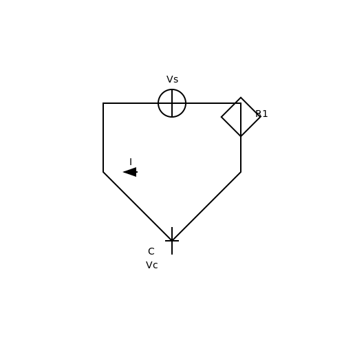
2. Understanding Closed Loops in Circuits
2.1 Understanding Closed Loops in Circuits
The foundation of Kirchhoff's Voltage Law (KVL) rests on the concept of closed loops within electrical circuits. A closed loop, or a circuit loop, is a complete path that allows electric current to flow continuously without any interruptions. When exploring KVL, it is crucial to understand the significance of these loops because they serve as key components in analyzing circuit behavior and performance.
In a closed loop, Kirchhoff's Voltage Law states that the sum of the electromotive forces (emf) and the voltage drops across all components must equal zero. This can be mathematically expressed as:
This signifies that the energy supplied by sources (like batteries) must be equal to the energy consumed by resistive elements (like resistors) within the loop. In practical terms, when we move around the loop, any rise in voltage (due to sources) counterbalances the drops caused by resistors or other components.
Identifying Closed Loops
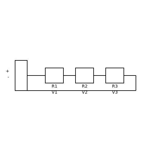
To effectively utilize KVL, one must skillfully identify closed loops within a circuit. Consider a simple series circuit containing a battery and three resistors connected in succession. This circuit forms a closed loop. If we apply KVL, we must assign a voltage drop for each component:
- Voltage Source: The voltage provided by the battery is counted as a positive value when traversing from the negative to the positive terminal.
- Resistors: The voltages across the resistors are typically treated as negative drops since they consume voltage as current passes through them.
Thus, conditionally traversing the circuit loop can guide us in setting up the corresponding equations using KVL. An insightful understanding of the circuit's topology is paramount because, in more complex configurations that include parallel branches or various types of components, the identification of closed loops becomes more intricate yet rewarding.
Practical Applications
In advanced electronics, KVL plays a vital role in planning and designing circuits used in diverse applications such as:
- Power Distribution Systems: Ensures that voltage levels across various components are maintained for efficient operation.
- Signal Processing: In communications, KVL assists in achieving proper signal integrity by ensuring consistent voltage levels through complex transmission lines.
- Feedback Circuits: KVL is essential in analyzing feedback mechanisms in operational amplifiers to stabilize and control circuit behavior.
Additionally, in experimental setups, validating KVL is crucial for verifying circuit efficiency and performance in research applications, such as investigating new materials for electrical applications.
In summary, understanding closed loops is instrumental when applying Kirchhoff’s Voltage Law. The insights gained from analyzing these loops not only deepen comprehension of circuit dynamics but also foster innovative designs and troubleshooting strategies in real-world scenarios.
2.2 Node Analysis Using KVL
In electrical circuit theory, Node Analysis using Kirchhoff's Voltage Law (KVL) is a powerful methodology for systematically analyzing circuits. This process not only aids in finding unknown voltages but also helps in understanding the interconnectivity and interactions among different components within the circuit.
To start with, it’s essential to recall that Kirchhoff's Voltage Law states that the sum of the electrical potential differences (voltages) around any closed network is zero. This principle is critical when establishing equations for various nodes in a circuit.
Understanding Node Analysis
Node Analysis revolves around the concept of identifying different nodes in a circuit and applying KVL around those nodes. A node is defined as any point where two or more circuit elements are interconnected. In applying KVL, we calculate the voltage drops across components connected to these nodes and sum them to equate to zero.
Let's consider a simple circuit consisting of resistors and a voltage source connected in series. The KVL provides a relationship for calculating voltages:
Where \( V \) is the source voltage, and \( V_1, V_2, \) and \( V_3 \) are the voltage drops across the resistors. If we define node voltages for different points in the circuit, we can formulate equations based on the KVL for each node.
Step-by-Step Calculation
Let's delve into a more structured approach to Node Analysis using KVL. The typical steps involved are as follows:
- Identify Nodes: Label all nodes in the circuit.
- Select a Reference Node: This can be grounded or any node assumed to have zero voltage.
- Write KVL Equations: For each node, apply KVL to determine the relationships between different voltages.
- Solve Equations: Utilize linear algebra techniques or computational tools to simultaneously solve for unknown voltages.
Example: Resistive Network Analysis
Consider a scenario with a resistive network where we have three nodes, with resistors \( R_1 \), \( R_2 \), and a voltage source \( V_s \) connected as shown below:
Label one node as A (where \( V_A \) is the voltage), and the reference node at ground potential (0 volts). Applying KVL to the loop yields:
Where \( I \) is the current through resistor \( R_1 \). This equation can be used in conjunction with Ohm's Law \( V = IR \) to depict relationships in the network further. Start substituting the corresponding values, and solve for the targeted voltages.
Practical Implications and Applications
Node analysis finds its relevance in numerous practical scenarios, such as:
- Electrical Engineering: Used extensively in circuit design and analysis.
- System Simulations: Helps in simulating complex networks in software applications like SPICE.
- Research and Development: Essential for experimenting with new circuit designs and validating theoretical principles.
This analytical approach not only simplifies circuit design challenges but also enhances comprehension of electrical systems, thereby facilitating efficient troubleshooting and optimization of circuit performance.
Mesh Analysis: A Step-by-Step Approach
Mesh analysis, also known as mesh current analysis, is a powerful technique in electrical engineering, particularly valuable in the analysis of planar circuits. By applying Kirchhoff's Voltage Law (KVL) around the loops of a circuit, this method allows us to formulate equations that define the behavior of the circuit based on the currents flowing through it. In this section, we will explore the mesh analysis process in detail through a systematic approach, showcasing its practical applications.
Understanding the Basics of Mesh Analysis
At its core, mesh analysis exploits the concept of mesh currents—hypothetical currents that circulate around a loop in a circuit. To effectively implement mesh analysis, it is important to follow a clear set of steps:
- Identify Meshes: Determine the number of independent loops within the circuit.
- Select Mesh Currents: Assign a mesh current for each independent loop, typically in a clockwise direction.
- Apply KVL: Write KVL equations for each mesh, expressing the sum of voltage drops as equal to voltage rises.
- Solve the System of Equations: Use algebraic methods to determine the unknown mesh currents.
Step-by-Step Process
1. Identifying Meshes
Begin by visually inspecting the circuit and labeling all the independent meshes. An independent mesh is defined as any loop that does not enclose any other loops. For example, consider a circuit consisting of three resistors and a voltage source:
2. Selecting Mesh Currents
For each independent mesh, select a direction for the mesh current. While the choice of direction is arbitrary, consistency is key throughout the analysis. Following our previous example, let’s denote the mesh currents as I1, I2, and I3.
3. Applying KVL
Next, apply KVL in each mesh, starting from any point in the loop and progressing around the loop until you return to the starting point. You need to consider voltage rises and drops based on the orientations of the components. For instance, in a mesh containing a voltage source and resistors, your KVL equation might appear as follows:
This equation states that the voltage rise from the source and the voltage drops across the resistors must tally to zero.
4. Solving the System of Equations
Once all equations are established, you will end up with a system of linear equations. These can be solved using methods such as substitution, elimination, or matrix inversion. For a simple circuit with two meshes, you might derive a system like:
Upon solving, you will obtain the mesh currents which can then be used to find voltages across components using Ohm's Law.
Practical Relevance and Application
Mesh analysis is particularly useful in circuit design and analysis within various fields such as telecommunications, embedded systems, and power distribution networks. Its ability to simplify complex circuits into manageable forms makes it indispensable for engineers and researchers. Notably, mesh analysis is often utilized in simulation software, allowing for rapid and accurate troubleshooting and optimization of electronic designs.
Case Study: Example Circuit
Consider a circuit with a 10V voltage source and two resistors of 5Ω and 10Ω. The setup consists of two meshes. To analyze such a circuit effectively using mesh analysis, follow the discussed steps systematically: identify meshes, assign currents, apply KVL, and solve for unknowns.
By accurately treating the resistive elements and validating each step, an engineer can gather insights about the overall circuit behavior, presently aligning current through each mesh and voltage levels across the resistors effectively.
Mesh analysis not only enhances comprehension of circuit dynamics but also prepares individuals for tackling real-world engineering challenges, blending theory with practical application.
3. KVL in Series Circuits
3.1 KVL in Series Circuits
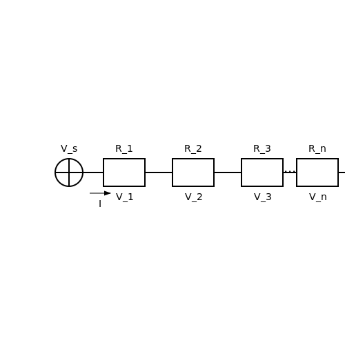
In the study of electrical circuits, Kirchhoff's Voltage Law (KVL) holds a paramount position, particularly when analyzing series circuits. At its core, KVL asserts that the sum of the electrical potential differences (voltages) around any closed network is zero. This law forms the foundation for understanding how voltage is distributed within a series circuit, a fundamental aspect of circuit design and analysis. When delving into series circuits, we recognize that components are connected end-to-end, allowing the same current to flow through each component. This crucial arrangement leads us to derive several key properties and relationships relevant to KVL.Understanding Series Circuits
In a series circuit, the total resistance, \( R_{\text{total}} \), can be expressed as the sum of individual resistances: $$ R_{\text{total}} = R_1 + R_2 + R_3 + \ldots + R_n $$ where \( R_1, R_2, \ldots, R_n \) represent the resistances of individual components. This concept is critical as it directly affects the voltage drop across each resistor, which is described by Ohm's Law: $$ V = IR $$ where \( V \) is the voltage, \( I \) is the current, and \( R \) is the resistance. Since current is uniform in a series circuit, we can express the voltage drop across each component. For each resistor \( R_i \), we have: $$ V_i = I \cdot R_i $$ where \( V_i \) represents the voltage across the \( i^{th} \) resistor.Applying KVL in Series Circuits
Applying KVL in a series circuit involves writing an equation that sets the sum of the voltage rises equal to the sum of the voltage drops. Consider a series circuit consisting of a voltage source \( V_s \) and multiple resistors \( R_1, R_2, \ldots, R_n \). According to KVL, we can write: $$ V_s - V_1 - V_2 - V_3 - \ldots - V_n = 0 $$ Substituting the expression for the voltage drops yields: $$ V_s - I \cdot R_1 - I \cdot R_2 - I \cdot R_3 - \ldots - I \cdot R_n = 0 $$ Factoring out the current \( I \) results in the elegant expression: $$ V_s - I \cdot (R_1 + R_2 + R_3 + \ldots + R_n) = 0 $$ From this equation, we can infer the current \( I \) in the circuit as: $$ I = \frac{V_s}{R_{\text{total}}} = \frac{V_s}{R_1 + R_2 + R_3 + \ldots + R_n} $$ This derivation highlights how KVL allows for the determination of current in response to the applied voltage and the network of resistances.Practical Relevance
The implications of KVL in series circuits extend far beyond theoretical analysis. Understanding this principle is vital in designing and troubleshooting real-world electronic systems, such as:- Battery packs: In applications where batteries are connected in series, KVL helps in assessing total voltage output and managing load distribution.
- Light bulb circuits: When bulbs are arranged in series, knowing how the voltage is divided among them can determine their brightness levels.
- Telecommunications: Series circuits are often employed in transmission lines, where KVL aids in minimizing voltage losses over distance.
3.2 KVL in Parallel Circuits
In parallel circuits, Kirchhoff's Voltage Law (KVL) manifests in intriguing ways, particularly as it pertains to the distribution of voltage across multiple paths. Building upon the foundational principles of KVL, which asserts that the sum of the electrical potential differences around a closed loop must equal zero, we can begin to explore the implications of this law in circuits where components are connected in parallel. In a parallel arrangement, each component is directly connected to the same two nodes. This configuration establishes a single voltage level across each branch, which significantly simplifies the application of KVL.Understanding Voltage Distribution
Let’s assume a parallel circuit with two branches containing resistors \( R_1 \) and \( R_2 \). Since they are connected in parallel, the voltage across each resistor is equal to the source voltage \( V_S \). In mathematical terms, we can express this as: $$ V_{R_1} = V_{R_2} = V_S $$ This equality suggests that no matter how the resistors differ in their resistance values, they will share the same voltage drop as long as they are connected across the same two points.Applying KVL in Parallel Circuits
Consider a more generalized parallel circuit containing \( n \) branches with varying resistances \( R_1, R_2, ..., R_n \). Each branch receives the same source voltage \( V_S \) as established above. When applying KVL around the loops formed in each branch of the parallel circuit, we can sum the voltages across each component: $$ \sum_{i=1}^n V_{R_i} = n V_S = 0 $$ In this case, since all individual voltages \( V_{R_i} \) equal \( V_S \), KVL confirms that the total potential "gains" (the source voltage in this case) equate to the total "drops," maintaining the essential equilibrium.Analyzing Current Flow in Parallel Circuits
It is crucial to recognize that while the voltage remains constant, the current flowing through each resistor might differ based on its resistance value, described by Ohm’s Law: $$ I_i = \frac{V_S}{R_i} $$ For our parallel network, the overall circuit current \( I_{total} \) can be calculated by summing the currents through each branch: $$ I_{total} = I_1 + I_2 + ... + I_n = \sum_{i=1}^n \frac{V_S}{R_i} $$ This formula is particularly useful in circuit design and analysis, where knowing how current is distributed can lead to improved efficiency and optimized performance. It lays the groundwork for understanding dynamic circuit responses, especially when resistors and other reactive components are introduced into the design.Real-World Applications
The principles of KVL in parallel circuits are prevalent in numerous applications. One of the most significant domains is within power distribution systems, where multiple loads operate independently while being fed from a common voltage source. This configuration enables flexibility in power management and improved reliability, as failure in one branch does not necessarily disrupt others. Similarly, parallel circuits are also extensively used in electronic devices. For instance, battery packs are typically arranged in parallel to enhance capacity while maintaining the same voltage level, allowing devices to run longer without increasing the circuit's voltage. In summary, KVL plays a fundamental role in analyzing parallel circuits. Its application not only simplifies complex calculations but also provides valuable insights into the behavior of electrical systems in real-world applications, thus bridging conceptual learning and practical engineering.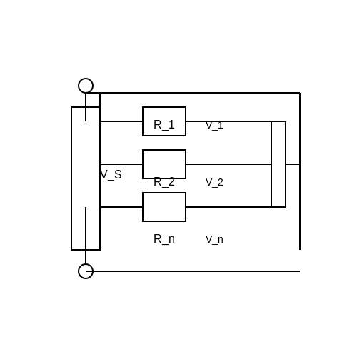
3.3 KVL in Complex Networks
In the exploration of electrical circuits, Kirchhoff's Voltage Law (KVL) serves as a foundational principle, essential for analyzing complex networks. When dealing with intricate arrangements—such as those found in multi-loop circuits, mesh analysis, or even combinations of series and parallel components—applying KVL demands a refined understanding of loop currents and voltage distributions.
KVL asserts that the algebraic sum of all voltages in a closed loop must be zero, a principle that can be extended to evaluate complex networks through systematic analysis. Specifically, loop analysis facilitates the examination of each independent loop while considering the contributions of resistive, capacitive, and inductive elements within the network.
Applying KVL in Mesh Analysis
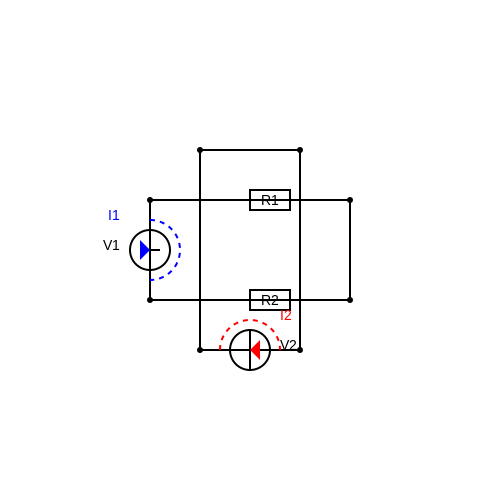
To systematically implement KVL in complex networks, mesh analysis offers a robust method. It involves defining a mesh current for each loop and writing KVL equations based on these mesh currents. Let us derive the equations through an example of a two-mesh network.
Consider two meshes in a network with resistors \( R_1 \), \( R_2 \) and voltage sources \( V_1 \), \( V_2 \). The current in the first mesh is \( I_1 \) and in the second mesh is \( I_2 \). Applying KVL to each mesh, we obtain:
These two equations can now be solved simultaneously for \( I_1 \) and \( I_2 \). Typically, one may rearrange the equations to isolate one current, then substitute back to find the values of both currents.
Practical Applications of KVL in Complex Networks
Understanding the application of KVL in complex networks is vital across various practical fields. Whether in the design of circuit boards, power distribution networks, or high-frequency communication systems, the ability to predict and analyze voltage drops and current flows proves indispensable. For example, in automotive electronics, accurate KVL analysis ensures that voltage divides correctly across numerous subsystems, thereby enhancing safety and reliability.
Furthermore, KVL plays a crucial role in developing algorithms for circuit simulation software. Advanced tools utilize KVL in conjunction with node voltage analysis to enable rapid simulations of circuit behavior, aiding engineers in refining designs before physical implementation.
In conclusion, while KVL provides a theoretical framework for voltage balance in electrical circuits, its implications in complex network analysis manifest profoundly in real-world applications, steering innovations in both circuit design and technology development.
4. Misapplications of KVL
4.1 Misapplications of KVL
In the exploration of Kirchhoff's Voltage Law (KVL), it is critical to recognize that misapplications can lead to significant errors in both theoretical predictions and practical implementations. KVL asserts that the sum of the electrical potential differences (voltages) around any closed network is zero. While powerful, its application demands a firm understanding of circuit elements and their configurations. One common misapplication of KVL occurs when neglecting the impact of non-ideal components, such as parasitic resistances and reactances prevalent in real-world circuits. For instance, when analyzing high-frequency circuitry, inductive and capacitive effects can introduce unforeseen impedances that KVL does not account for in a simplified framework. This oversight can lead to erroneous voltage readings and ultimately malfunctioning circuits. Additionally, KVL is often incorrectly employed in loop analysis where the direction of the assumed current does not align with the actual current flow. A classic case involves sign conventions; when assigning polarities to voltage sources and drops, a lack of consistency can yield contradictory results. For example, in a circuit with multiple power supplies, incorrectly gauging the rise and drop in potential due to inconsistency in loop traversal direction could lead to a sum that does not equal zero. Moreover, KVL cannot be applied effectively in circuits under dynamic conditions without considering time-dependent factors. In the case of circuits involving capacitors or inductors, voltages can vary with time, necessitating a focus on average values or instantaneous values depending on the applicable context, particularly in feedback systems where stability is essential. Another misapplication arises in analysis involving capacitive or inductive coupling. The interaction between components can manifest unexpected voltage drops due to mutual inductance or capacitive coupling effects, which are not captured by KVL in isolation. Thus, misinterpretations can lead to underestimating or overestimating voltage across elements in integrated circuits. These misapplications highlight the necessity of integrating KVL within a broader analytical framework that includes an understanding of component behavior, especially under real-world operating conditions. Recognizing these pitfalls is crucial for advanced circuit designers, researchers, and engineers striving for accuracy in their work. Practical applications of understanding these misapplications are extensive. For instance, in the design of amplifiers or filters, evaluating the role of parasitic elements and coupling in real circuits can lead to performance improvements and reliability. Meanwhile, in the realm of power systems, recognizing KVL's limitations aids in proper network analysis, ensuring adequate supply and stability across the grid. In closing, while KVL serves as a fundamental tool in electrically analyzing circuits, its effective application requires awareness of the conditions and assumptions underlying its use. By recognizing common misapplications, professionals can bridge theory with practical implementation, steering clear of pitfalls that could compromise circuit functionality.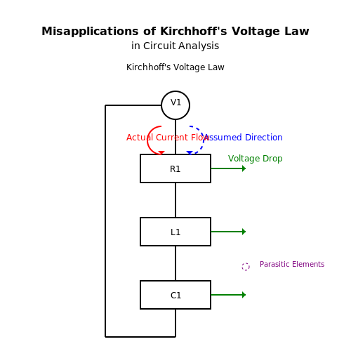
4.2 Understanding Voltage Drops and Sources
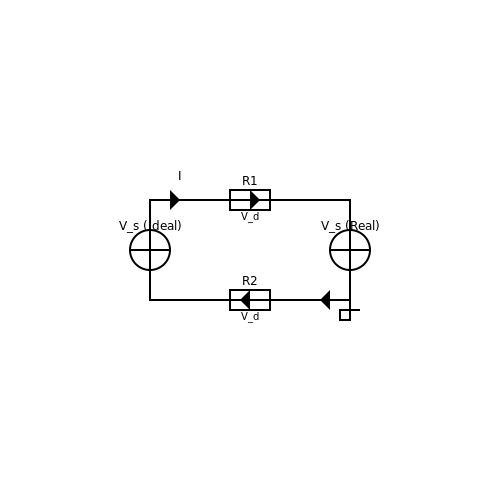
In the context of each electrical circuit, the application of Kirchhoff's Voltage Law (KVL) is significantly intertwined with the concepts of voltage drops and sources. Understanding these phenomena is essential for analyzing complex circuits and ensuring functional integrity in electronic designs. This subsection aims to elucidate the fundamental principles governing voltage drops and sources, alongside their implications in real-world applications.
Defining Voltage Drops
Voltage drop refers to the decrease in electrical potential along a conductor or across a component when current flows through it. This phenomenon can be attributed to the inherent resistance of materials and components that characterizes every physical circuit. The relationship between current, resistance, and voltage drop is encapsulated in Ohm's Law, which states:
where:
- $$ V_d $$ = Voltage drop (in volts)
- $$ I $$ = Current flowing through the component (in amperes)
- $$ R $$ = Resistance of the component or conductor (in ohms)
This equation shows that the voltage drop is directly proportional to both the current passing and the resistance of the component. In practical applications, understanding the voltage drop across various components is crucial, particularly in power distribution systems, where ensuring minimal voltage drop is essential for effective energy delivery.
Exploring Voltage Sources
Voltage sources, on the other hand, are components that provide a consistent voltage level to the circuit. They can be classified broadly into two types: ideal and real voltage sources. An ideal voltage source maintains a constant voltage regardless of the current drawn, while a real voltage source has internal resistance that affects its output voltage when subjected to varying loads. This behavior leads to a more complex relationship between voltage and current, particularly for real-world applications.
The characteristics of voltage sources can be represented via the source's voltage ($$ V_s $$) in a circuit, which adds to the overall voltage around a closed loop, as stated by KVL:
where the sum of voltage sources ($$ V_s $$) minus the sum of the voltage drops ($$ V_d $$) in a loop equals zero. This principle is essential in ensuring that the total energy provided by sources is balanced by the energy consumed by the components within a circuit.
Practical Implications and Applications
In engineering and research contexts, analyzing voltage drops and sources is pivotal for several reasons:
- Power System Analysis: Engineers must consider voltage drops while designing power distribution networks to maintain efficiency and minimize losses.
- Circuit Performance Tuning: Voltage sources with different internal resistances can significantly affect circuit behavior. Understanding this allows engineers to choose appropriate components for desired performance.
- Safety and Compliance: Certain applications, particularly in critical infrastructure, require strict adherence to voltage specifications to prevent equipment damage or failure.
A practical example includes digital circuits where voltage levels dictate binary states (high or low). Engineers must ensure that voltage drops across paths do not interfere with logic signals.
This section established a detailed grounding in the principles of voltage drops and sources, reinforcing their importance within the framework of Kirchhoff's Voltage Law. Moving forward, we will delve deeper into analyzing complex circuits using these foundational concepts.
4.3 Troubleshooting KVL in Circuit Designs
The application of Kirchhoff's Voltage Law (KVL) in circuit design is foundational to electrical engineering, enabling engineers to analyze and optimize circuits effectively. This subsection delves into troubleshooting KVL in circuit designs by providing advanced techniques and methodologies that are essential for identifying and resolving discrepancies between theoretical predictions and practical outcomes.
Understanding Common Challenges
When implementing KVL, engineers may encounter several common challenges such as:
- Measurement Errors: Inaccurate voltage readings can arise from faulty instruments or improper setup, leading to significant discrepancies in KVL application.
- Component Non-Idealities: Real-world components do not behave as perfect ideal components. For example, resistors have tolerances, and capacitors may exhibit leakage, affecting the voltage distribution in the circuit.
- Grounding Issues: Poor grounding can introduce noise and potential differences that distort KVL results.
Systematic Troubleshooting Approach
To address these challenges systematically, follow a structured approach:
1. Verify Circuit Connections
Ensure all connections are secure and correct according to the schematic. Incomplete or loose connections can lead to unexpected voltage drops and current paths. Use a continuity tester to confirm connections.
2. Measure Voltages at Key Points
Employ a digital multimeter (DMM) to accurately measure the voltage across each component in the circuit. Record your measurements and compare them against the expected values derived from KVL calculations. A systematic approach includes:
- Measuring the voltage across each resistor and comparing it with Ohm’s Law.
- Tracking voltage drops across non-linear components like diodes and transistors.
3. Analyze Component Behavior
Assess each component's specifications against the circuit’s operating conditions. For instance, an inoperative capacitor can cause an increase in voltage across other components, breaking KVL. Understanding the Voltage-Current (V-I) characteristics of devices is crucial at this stage.
4. Re-evaluate Grounding and Reference Points
Inspect the grounding layout and reference potentials. A solid ground reference minimizes noise and helps in achieving accurate voltage readings. Consider using multiple ground points to mitigate ground loops, particularly in complex circuits.
5. Simulate Circuit Behavior
Utilize circuit simulation software such as SPICE to model the circuit and observe theoretical voltage behaviors. This enables the identification of discrepancies between simulation results and actual measurements, often highlighting overlooked factors or errors.
Advanced Techniques: Using KVL in Feedback Analysis
Another effective method to ensure compliance with KVL in design is by implementing feedback analysis. Feedback loops can stabilize circuit parameters by dynamically adjusting operating conditions based on voltage discrepancies. This is particularly relevant in active control systems where maintaining a specific voltage level is critical. To apply feedback mechanisms:
- Design a feedback loop with operational amplifiers to continuously monitor output voltage.
- Use PID (Proportional-Integral-Derivative) controllers for effective adjustment and control of circuit outputs.
Through the application of these troubleshooting techniques and methodologies, one can enhance the accuracy of KVL applications within circuit designs, leading to more reliable and robust electrical systems. Understanding these challenges and solutions not only emphasizes the importance of KVL but also equips engineers with tools to refine their circuit designs effectively.
5. KVL in AC Circuits
5.1 KVL in AC Circuits
Kirchhoff's Voltage Law (KVL) remains a fundamental principle in analyzing electrical circuits, encompassing both direct current (DC) and alternating current (AC) scenarios. Applying KVL in AC circuits necessitates an understanding of reactive components and phase relationships, which introduce complexity compared to their DC counterparts. In this subsection, we will explore how KVL operates within AC circuits, enriching our understanding of reactive elements like inductors and capacitors, and how they impact voltage distribution and phase.
Understanding AC Circuits
Alternating current (AC) differs from direct current (DC) primarily in its characteristics: voltage and current vary sinusoidally over time rather than remaining constant. Through this oscillation, AC systems deliver power more efficiently over long distances. When analyzing AC circuits, components such as resistors (R), inductors (L), and capacitors (C) exhibit unique behaviors defined by their impedance, measured in ohms. The impedance \(Z\) of a component modifies KVL as follows:
Here, \(j\) represents the imaginary unit, and \(X\) denotes the reactance, which varies based on frequency.
Applying KVL in AC Circuits
KVL states that the sum of the electrical potential differences (voltage) around any closed network is zero. In AC circuits, this summation incorporates both resistive and reactive impedances. When applying KVL, voltages across resistors, inductors, and capacitors must be considered in their complex forms.
For instance, take a simple series AC circuit consisting of a resistor \(R\), an inductor \(L\), and a capacitor \(C\). The total voltage \(V\) across this network can be represented as:
Where:
- Voltage across the resistor: \( V_R = I \cdot R \)
- Voltage across the inductor: \( V_L = I \cdot j\omega L \)
- Voltage across the capacitor: \( V_C = \frac{I}{j\omega C} \)
In these equations, \(I\) is the current flowing through the circuit, and \(\omega\) is the angular frequency of the AC source. These voltages can be expressed in the phasor domain, where amplitudes and phase angles become more manageable.
Practical Relevance and Applications
Understanding KVL in AC circuits is not merely academic; it has extensive real-world implications. Engineers frequently use these principles when designing power systems, electronic devices, and telecommunications equipment. For example, in designing a resonant circuit for RF applications, KVL helps predict how components will behave at various frequencies, ensuring optimal performance.
Moreover, in the context of renewable energy, applying KVL in AC circuits is essential for integrating solar panels and wind turbines into the grid, where complex interactions between various circuit elements must be carefully managed to maintain voltage stability.
As we conclude this section, we recognize that applying KVL in AC circuits enriches our analytical tools, enabling robust design and evaluation of a wide variety of AC-based systems.
5.2 Impact of Non-Linear Components
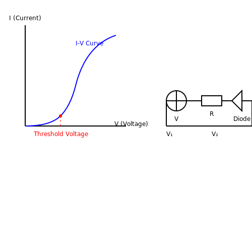
In electrical circuits, Kirkhoff's Voltage Law (KVL) is foundational for understanding the relationship between potential differences around a closed loop. While KVL holds true for both linear and non-linear components, the behavior and analysis of non-linear components introduce complexities that deviate from conventional linear models. This subsection will explore how non-linear components, including diodes, transistors, and other devices, impact circuit behavior, including implications for KVL.
The Nature of Non-Linear Components
Non-linear components are those whose current-voltage (I-V) characteristics do not follow a linear relationship. For instance, a diode exhibits an exponential I-V relationship defined by the Shockley equation:
Here, I is the current, Is is the saturation current, q is the charge of an electron, V is the voltage across the diode, k is Boltzmann's constant, and T is the absolute temperature in Kelvin. This equation highlights how diodes conduct significantly more current at higher voltages due to their exponential nature, leading to significant implications when applying KVL.
Challenges in Applying KVL with Non-Linear Components
When applying KVL in circuits involving non-linear components, one encounters the need for iterative solutions or graphical analysis techniques. The challenge arises because, unlike linear components (such as resistors), whose voltage and current can be directly related through Ohm's Law, non-linear devices require a different approach. For example:
- Piecewise Analysis: Given that non-linear components can have multiple operating states, it may be beneficial to break down the circuit into regions where non-linear characteristics can be treated as linear.
- Simulation Techniques: Tools such as SPICE provide a platform for simulating non-linear circuits, taking into account the varying characteristics of components across different operating points.
This leads to the necessity for iterative techniques or numerical methods to solve KVL equations involving these components. Each iteration may recognize how the non-linear properties alter the total voltage around the loop, as seen in more advanced methods like the Newton-Raphson method for obtaining voltage values at different points in the circuit.
Real-World Applications and Implications
The implications of non-linear components become especially pronounced in scenarios such as:
- Switching Power Supplies: These circuits utilize non-linear devices for regulating output voltage. KVL is pivotal when calculating feedback loops that rely on nonlinear behavior to maintain target output.
- Signal Processing: In RF circuits and communication systems, non-linear components like amplifiers are essential, requiring KVL to address distortion effects accurately.
- Control Systems: Non-linear control systems necessitate applying KVL in their analysis to ensure system stability, particularly in systems that engage with snap-action devices like relays.
Understanding the implications of non-linear components on KVL is thus crucial for designing robust circuits capable of operating reliably in real-world conditions.
In conclusion, while KVL remains a cornerstone principle in circuit analysis, the intricacies and behaviors of non-linear devices necessitate an expansion of analytical techniques. By combining theoretical knowledge with practical application, engineers can effectively design and analyze complex circuits that utilize these vital non-linear components.
5.3 KVL and Operational Amplifiers
Kirchhoff's Voltage Law (KVL) forms the backbone of circuit analysis and is particularly critical when analyzing operational amplifiers (op-amps). An op-amp is a versatile electronic device widely used in signal conditioning, filtering, and mathematical operations. Understanding the application of KVL in op-amps enhances not just theoretical comprehension but also practical circuit design skills.
Operational amplifiers are designed to amplify difference voltages between their inverting (\(V_-\)) and non-inverting (\(V_+\)) inputs. The ideal op-amp is characterized by infinite input impedance (which means it draws no current), zero output impedance, and infinite gain. In real-world applications, these characteristics can vary, but KVL still applies for comprehensive circuit analysis.
Understanding KVL in Op-Amp Circuits
To analyze a circuit using a KVL approach, it’s essential to recognize the virtual short concept in ideal op-amps. This means that due to the high gain of the amplifier, the voltages at the two input terminals are virtually equal in steady state. Thus, if we denote the output voltage as \(V_{out}\) and the input voltages coming into the op-amp as \(V_+\) and \(V_-\), KVL can be applied effectively in the surrounding circuit paths.
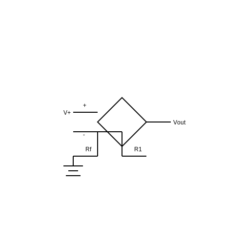
Consider the following basic setup for a non-inverting op-amp configuration:
Non-Inverting Op-Amp Configuration:
- Let \(R_1\) be the resistor from the output \(V_{out}\) to the inverting input \(V_-\).
- Let \(R_f\) be the feedback resistor connecting the inverting input \(V_-\) to ground.
Applying KVL around the loop formed by \(V_{out}\), \(R_1\), and the two inputs gives:
Substituting \(V_-\) with \(V_+\) (using the virtual short assumption), we can rewrite this as:
This equation illustrates how the output voltage of a non-inverting op-amp is related to its input voltage \(V_+\) and the resistor values \(R_1\) and \(R_f\). The gain of this configuration is therefore:
Practical Applications and Implications
The relationship established by the equations derived above is crucial in designing amplifiers for various applications, including:
- Signal amplification: Used in audio systems to enhance weak signals.
- Filters: Op-amps can construct active filters to isolate frequency components.
- Integrators and Differentiators: Signal processing and mathematical operations in control systems.
In each of these examples, KVL aids in analyzing the input-output relationships effectively, allowing engineers to predict circuit behavior with accuracy. The interaction between resistors, capacitors, and the op-amp dynamics illustrates the fundamental principles of circuit theory and helps in designing efficient electronic systems.
Bringing KVL into practical circuit elements not only solidifies theoretical knowledge but also paves the way for innovative designs in modern electronics.
6. Textbooks on Circuit Analysis
6.1 Textbooks on Circuit Analysis
An Introduction to Circuit Analysis through Textbooks
Circuit analysis is a foundational subject in electrical engineering and is crucial for understanding how electrical circuits function. For those exploring applied aspects of Kirchhoff's Voltage Law (KVL), having a strong grasp on circuit analysis is essential. The following textbooks provide comprehensive coverage of circuit analysis principles, including KVL. They serve as excellent references for both students and professionals seeking depth in understanding and application.Recommended Textbooks
- Introductory Circuit Analysis by Robert L. Boylestad — This book is renowned for its clear presentation of essential circuit analysis concepts, including KVL, making it accessible for beginners. It incorporates practical examples and problem-solving techniques useful for both classroom and real-world applications.
- Circuit Analysis: Theory and Practice by Allan H. Robbins and Wilhelm C. Miller — Known for its extensive use of examples and practical applications, this textbook is ideal for advanced learners. It covers KVL thoroughly, integrating technology and software tools to accomplish complex analysis tasks.
- Fundamentals of Electric Circuits by Charles K. Alexander and Matthew N.O. Sadiku — This book provides an engaging approach to learning circuit analysis with rich problem-solving contexts. Every chapter enhances the understanding of KVL through comprehensive examples and practice problems.
- Basic Engineering Circuit Analysis by J. David Irwin and R. Mark Nelms — Offering a balanced exposition of theory and practice, this book addresses KVL with detailed coverage of methods and applications. It is notably helpful for students who appreciate a step-by-step learning approach.
- Electric Circuits by James W. Nilsson and Susan A. Riedel — This textbook stands out for its systematic approach to enhancing intuition in circuit analysis practices, such as KVL. Its clear narrative and innovative problem sets make it a comprehensive guide for learners.
- Introduction to Electric Circuits by Richard C. Dorf and James A. Svoboda — This book covers the building blocks of circuit theory, with detailed explorations of KVL concepts. The authors blend explanations with practical applications, complemented by available online resources for enhanced learning.
- Network Analysis and Synthesis by Franklin F. Kuo — A seminal text in its own right, this book delves deeply into network analysis, offering substantial treatment of KVL in the context of electrical networks. It is particularly suited for advanced postgraduate studies and research.
6.2 Academic Journals and Papers
- IEEE Xplore: Kirchhoff's Voltage Law in Circuit Theory — This paper provides a detailed exploration of Kirchhoff's Voltage Law with a focus on its application in circuit theory, discussing both historical perspectives and modern computational techniques.
- ScienceDirect - Application of Kirchhoff's Laws in Network Analysis — This study investigates novel applications of Kirchhoff's laws in electrical network analysis and provides insights into solving complex circuits using computational methods.
- SAGE Journals: A New Perspective on Kirchhoff’s Laws — Offers a fresh perspective on the fundamental principles of Kirchhoff’s Laws, integrating both engineering and physics viewpoints with comprehensive analytical discussions.
- American Journal of Physics - Teaching Kirchhoff's Laws — Discusses effective pedagogical strategies for teaching Kirchhoff’s laws with an emphasis on practical hands-on circuit experiments and simulations.
- Springer: Kirchhoff's Laws in Nanoscale Devices — Explores the relevance of Kirchhoff's laws in the context of nanoscale electronic devices, offering insights into current challenges and innovations.
- IEEE Author Center - Understanding Peer Review — A guide to navigating the peer review process in academic publishing, invaluable for researchers submitting work related to Kirchhoff's laws.
- MDPI Electronics: Extended Kirchhoff’s Laws and Superconducting Circuits — This publication delves into extensions of Kirchhoff’s laws applicable to superconducting circuits and how they can be utilized in quantum computing applications.
6.3 Online Resources and Tutorials
For those seeking a deeper understanding of Kirchhoff's Voltage Law (KVL) and its applications in complex electrical circuits, there exist numerous high-quality resources and tutorials available online. Below is a curated list of some of the most effective online resources to aid your study, featuring comprehensive explanations, practical examples, and interactive simulations.- Khan Academy: DC Circuit Analysis — This resource provides a detailed explanation of Kirchhoff's Laws, including KVL, with video lectures and practice problems designed for in-depth understanding.
- Electronics Tutorials: Kirchhoff's Voltage Law — Offers a comprehensive guide on KVL with step-by-step derivations of key principles and real-world circuit examples.
- CircuitLab: Understanding Kirchhoff's Laws — An interactive platform where users can simulate electrical circuits and apply KVL practically to see theoretical concepts in action.
- MIT OpenCourseWare: Circuits and Electronics — This course includes lecture notes and assignments on circuits, providing an academic perspective on KVL and its applications.
- Electrical4U: Kirchhoff's Laws — A resource for both beginners and experts featuring detailed discussions of KVL with practical problem-solving techniques.
- All About Circuits: Kirchhoff's Laws — Provides a deep dive into Kirchhoff's Laws with text, illustrations, and solved examples that enhance comprehension.
- SparkFun: Voltage, Current, Resistance, and Ohm's Law — While not exclusively about KVL, this tutorial sets the foundation upon which KVL is understood, especially useful for reinforcing fundamental concepts.