Zero-Phase Error Tracking Systems
1. Definition and Core Principles
1.1 Definition and Core Principles
A zero-phase error tracking system is a control architecture designed to eliminate phase lag between a reference signal and the system's output response. This is achieved through precise compensation techniques that ensure the output precisely aligns with the input in both amplitude and phase across the operating bandwidth. Such systems are critical in applications where temporal alignment is paramount, such as high-precision motion control, phased-array radar, and optical coherence tomography.
Mathematical Foundation
The core principle relies on the frequency-domain representation of the system's transfer function G(s). For zero-phase error, the system must satisfy:
where ωc is the cutoff frequency. To achieve this, the system typically employs a phase-lead compensator or a feedforward path that cancels the inherent phase lag of the plant dynamics. The compensator transfer function C(s) is designed such that:
Key Components
- Reference Model: Generates the ideal trajectory or signal that the system must track with zero phase error.
- Phase Compensator: Dynamically adjusts the system's phase response to cancel lag introduced by inertial or capacitive elements.
- Feedback Loop: Measures the output phase error and corrects it in real-time through adaptive control.
Practical Implementation
In digital implementations, a common approach uses a finite impulse response (FIR) filter with symmetric coefficients to ensure linear phase. The filter's group delay τg is constant across all frequencies, given by:
where N is the filter length. This property is exploited in applications like real-time signal processing where phase distortion must be minimized.
Historical Context
The concept originated in the 1970s with the development of repetitive control systems for disk drive head positioning, where sub-micron tracking accuracy required elimination of phase lag. Modern applications extend to quantum control systems and gravitational wave detectors, where attosecond-scale timing is critical.
Performance Metrics
System quality is quantified by:
- Phase Margin: Typically > 60° for robust zero-phase operation
- Bandwidth: The frequency range where |∠G(jω)| < 1°
- Tracking Error: RMS phase deviation in microradians

1.2 Importance in Control Systems
Zero-phase error tracking systems are critical in control applications where temporal alignment between reference signals and system responses is paramount. Phase distortions introduce lag or lead, degrading performance in precision tasks such as robotic motion control, active noise cancellation, and high-speed servo systems. The absence of phase error ensures that the system's output precisely mirrors the input in time, a requirement for stability and accuracy in feedback loops.
Phase Sensitivity in Feedback Systems
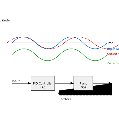
In a closed-loop control system, phase errors accumulate through cascaded components (e.g., sensors, filters, actuators). Consider a PID controller with transfer function:
A phase lag introduced by the plant dynamics \( G(s) \) shifts the system's crossover frequency, risking instability. Zero-phase error compensators, such as non-causal FIR filters, correct this by applying a symmetric impulse response:
This symmetry guarantees zero group delay, preserving the temporal integrity of the reference trajectory.
Applications in Real-Time Systems
In hard real-time systems (e.g., CNC machines, radar tracking), phase misalignment directly translates to positional errors. For instance, a robotic arm following a sinusoidal path with phase lag \( \phi \) exhibits a tracking error \( \Delta x \):
Zero-phase filtering, implemented via forward-backward filtering or phase-locked loops (PLLs), eliminates \( \phi \), achieving sub-millisecond synchronization.
Case Study: Active Vibration Control
Aerospace systems use zero-phase tracking to cancel vibrations in real time. A feedforward controller with a zero-phase adaptive filter (e.g., FxLMS algorithm) measures vibrations \( d(t) \) and generates an anti-phase signal \( y(t) \). The cancellation condition:
requires \( y(t) \) to align perfectly with \( d(t) \), necessitating zero-phase error.
Mathematical Derivation: Zero-Phase FIR Design
Design a linear-phase FIR filter of order \( N \) (even) with coefficients \( b_k \). For zero phase, impose symmetry \( b_k = b_{N-k} \). The frequency response \( H(e^{j\omega}) \) becomes:
where \( a_k = 2b_{N/2-k} \) for \( k > 0 \). The term \( e^{-j\omega N/2} \) represents a constant delay, removable via time-domain shifting.
1.3 Key Performance Metrics
Phase Error and Tracking Accuracy
The primary metric for zero-phase error tracking systems is the phase error (φe), defined as the difference between the reference signal phase and the system's output phase. For an ideal zero-phase system:
In practice, phase error arises from system non-idealities such as loop delay, quantization effects, and component tolerances. The root-mean-square (RMS) phase error provides a statistical measure of tracking accuracy:
Bandwidth and Settling Time
The closed-loop bandwidth (ωc) determines how rapidly the system can track phase variations. For a second-order phase-locked loop (PLL), the bandwidth relates to natural frequency (ωn) and damping ratio (ζ):
Settling time (ts), the duration required for phase error to converge within a specified tolerance (typically 1% or 5%), is critical for applications like clock synchronization:
Jitter and Phase Noise
Timing jitter quantifies short-term phase variations, typically measured in picoseconds RMS. In frequency domain, phase noise (L(f)) characterizes spectral purity:
where Pnoise(f) is the noise power at offset frequency f from the carrier, and Pcarrier is the total signal power. Advanced systems achieve phase noise below -100 dBc/Hz at 1 kHz offset.
Dynamic Range and Linearity
The tracking range defines maximum input frequency deviation the system can follow without losing lock. For digital implementations, the effective number of bits (ENOB) of phase detectors impacts linearity:
where SINAD is the signal-to-noise-and-distortion ratio. High-performance systems maintain ENOB > 12 bits across the operating range.
Stability Metrics
Phase margin (PM) and gain margin quantify stability robustness. For zero-phase systems, phase margin exceeding 45° ensures adequate damping:
where G(s) and H(s) are the open-loop transfer functions. Modern implementations use Lyapunov exponents for nonlinear stability analysis.
2. Phase Error Analysis
2.1 Phase Error Analysis
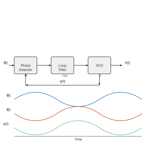
Phase error in tracking systems arises when the output signal's phase deviates from the reference signal's phase, leading to misalignment in control or measurement applications. The phase error φ(t) is defined as the difference between the input phase θref(t) and the output phase θout(t):
In frequency-domain analysis, phase error is often characterized by the transfer function H(s) of the phase-locked loop (PLL) or tracking system. The open-loop phase transfer function for a second-order PLL is given by:
where Kv is the VCO gain, Kp is the phase detector gain, and F(s) is the loop filter transfer function. The steady-state phase error for different input signals can be derived using the final value theorem:
Sources of Phase Error
The primary contributors to phase error in tracking systems include:
- Loop delay: Propagation delays in feedback paths introduce phase lag.
- Nonlinearities: Saturation in amplifiers or phase detectors distorts the error signal.
- Noise: Thermal and flicker noise in oscillators cause jitter.
- Frequency drift: Variations in reference or VCO frequency over time.
Phase Error Compensation Techniques
To minimize phase error, several compensation strategies are employed:
- Lead-lag filters: Adjust loop dynamics to improve phase margin.
- Adaptive bandwidth control: Dynamically adjusts loop bandwidth to balance noise rejection and tracking speed.
- Digital phase interpolation: Used in all-digital PLLs for fine phase correction.
Practical Implications
In high-precision applications such as radar, optical coherence tomography, and synchronous sampling, phase errors below 0.1° are often required. Advanced techniques like sub-sampling phase detectors and time-to-digital converters (TDCs) achieve sub-picosecond jitter performance.
where σφ is the RMS phase noise, F is the noise figure, k is Boltzmann's constant, T is temperature, and Psig is the signal power.
2.2 Transfer Functions and Stability Criteria
The transfer function of a zero-phase error tracking system provides a mathematical representation of its dynamic behavior in the frequency domain. For a linear time-invariant (LTI) system, the transfer function G(s) is defined as the ratio of the Laplace transform of the output to the Laplace transform of the input, assuming zero initial conditions:
where Y(s) is the output signal, U(s) is the input signal, and s is the complex frequency variable. The poles and zeros of G(s) determine the system's stability and transient response.
Pole-Zero Analysis
The poles of G(s) are the roots of the denominator polynomial, while the zeros are the roots of the numerator polynomial. For a system to be stable, all poles must lie in the left half of the complex plane (i.e., have negative real parts). A zero-phase error tracking system must ensure that the phase response remains minimal across the operating bandwidth, which imposes additional constraints on pole-zero placement.
where zi are the zeros and pi are the poles. If any pole has a positive real part, the system becomes unstable, leading to unbounded output growth.
Nyquist and Bode Stability Criteria
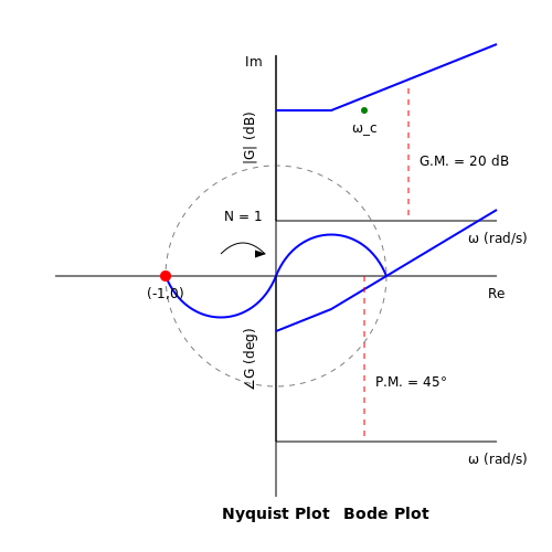
The Nyquist stability criterion assesses stability by examining the encirclement of the critical point (-1, 0) in the complex plane by the Nyquist plot of G(s). For a stable system, the number of clockwise encirclements must equal the number of right-half-plane poles of the open-loop transfer function.
In contrast, the Bode stability criterion evaluates phase and gain margins from the Bode plot. A sufficient phase margin (typically > 45°) and gain margin (typically > 6 dB) ensure robustness against parameter variations and disturbances.
Practical Stability Considerations
In real-world implementations, non-ideal components, delays, and nonlinearities can introduce additional poles or phase shifts. For zero-phase error tracking, compensation techniques such as lead-lag networks or phase-locked loops (PLLs) are often employed to correct phase deviations while maintaining stability.
For example, a second-order system with a transfer function:
must have a damping ratio ζ > 0 to ensure stability. Underdamped systems (ζ < 1) exhibit oscillatory responses, while critically damped (ζ = 1) and overdamped (ζ > 1) systems converge without oscillation.
Routh-Hurwitz Criterion
For higher-order systems, the Routh-Hurwitz criterion provides a systematic method to determine stability without explicitly solving for the poles. By constructing the Routh array from the coefficients of the characteristic polynomial, the number of right-half-plane poles can be deduced from sign changes in the first column.
Consider a third-order system with the characteristic equation:
The Routh array is constructed as:
| Row | Column 1 | Column 2 |
|---|---|---|
| 1 | 1 | a1 |
| 2 | a2 | a0 |
| 3 | b1 = (a2a1 - a0) / a2 | 0 |
| 4 | a0 | 0 |
The system is stable if all elements in the first column are positive.
2.3 Frequency Domain Representation
The frequency domain representation of a zero-phase error tracking system provides critical insights into its stability, bandwidth, and dynamic response. By analyzing the system's transfer function in the frequency domain, we can quantify phase distortion and ensure minimal tracking error.
Transfer Function Analysis
Consider a zero-phase error tracking system with a closed-loop transfer function H(s). In the frequency domain, we substitute s = jω, yielding:
where Y(jω) is the output spectrum and R(jω) is the reference input spectrum. The magnitude and phase response are given by:
For zero-phase error, ϕ(ω) must remain as close to zero as possible across the operational bandwidth.
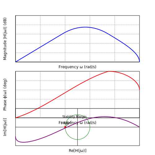
Bode Plot Interpretation
A Bode plot visualizes the magnitude (in dB) and phase (in degrees) of H(jω) as a function of frequency. For an ideal zero-phase system:
- The magnitude plot should exhibit a flat response within the desired bandwidth.
- The phase plot should remain near zero degrees, indicating minimal phase lag.
Deviations from this ideal behavior reveal phase distortion, which can be corrected using phase compensation techniques such as all-pass filters or predictive control.
Nyquist Stability Criterion
The Nyquist plot, which maps H(jω) in the complex plane, provides a stability assessment. For a zero-phase system:
where P is the number of unstable poles of the open-loop system and Z is the number of unstable closed-loop poles. Zero-phase systems must ensure Z = 0 for stability.
Practical Applications
In high-precision motion control systems, such as robotic arms or CNC machines, frequency domain analysis ensures that the tracking system maintains phase coherence. For example, in optical tracking systems, phase errors can lead to misalignment, which is mitigated by optimizing the system's frequency response.
Modern implementations often employ digital signal processing (DSP) techniques, where the discrete-time Fourier transform (DTFT) is used to analyze and correct phase errors in real time.
3. System Architecture
3.1 System Architecture
The architecture of a zero-phase error tracking system is designed to eliminate phase lag between the reference signal and the system output, ensuring precise synchronization in dynamic control applications. At its core, the system integrates a feedback loop with predictive compensation to correct phase distortions in real time.
Core Components
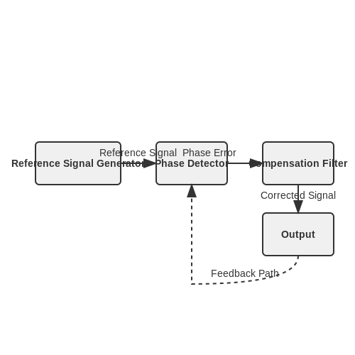
The system consists of three primary modules:
- Reference Signal Generator — Produces the target waveform (e.g., sinusoidal, square, or arbitrary) with minimal jitter.
- Phase Detector — Compares the input and output signals to quantify phase discrepancies. Common implementations use XOR gates or mixers for high-frequency applications.
- Compensation Filter — A finite impulse response (FIR) or adaptive filter that adjusts the system's response to nullify phase errors.
Mathematical Foundation
The phase error φ is derived from the time delay Δt between signals:
where f is the signal frequency. To achieve zero-phase error, the compensation filter applies a gain G(ω) and phase shift θ(ω) such that:
where H(ω) is the plant transfer function. For a causal system, this requires:
Implementation Techniques
Two dominant approaches are:
- Feedforward Correction — Pre-distorts the reference signal using an inverse model of the plant.
- Feedback Adaptive Control — Dynamically adjusts filter coefficients via LMS (Least Mean Squares) or RLS (Recursive Least Squares) algorithms.
Practical Considerations
Nonlinearities in actuators and sensors introduce higher-order harmonics, necessitating:
- Over-sampling (≥10× Nyquist rate) to mitigate aliasing.
- Kalman filters for noise suppression in low-SNR environments.
3.2 Component Selection and Tuning
Critical Components for Zero-Phase Error Systems
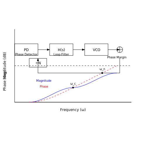
The performance of a zero-phase error tracking system hinges on the precise selection of its core components: phase detectors, loop filters, voltage-controlled oscillators (VCOs), and feedback dividers. Each component must be chosen to minimize phase drift and maintain stability under dynamic conditions.
- Phase Detectors: A multiplier-based or XOR phase detector is often preferred for its linearity over a limited range. For high-precision applications, a phase-frequency detector (PFD) with dead-zone elimination ensures minimal static phase error.
- Loop Filters: The filter's bandwidth and order dictate the system's transient response. A second-order active proportional-integral (PI) filter is common, with its transfer function given by:
where τ1 and τ2 are time constants derived from the desired damping ratio (ζ) and natural frequency (ωn).
Tuning Methodology
The loop bandwidth (ωc) must balance noise rejection and tracking speed. For a second-order system, the relationship between ωc, ωn, and ζ is:
Practical tuning involves:
- Step 1: Set ζ to 0.707 (critical damping) for optimal transient response.
- Step 2: Adjust ωn to position the loop bandwidth below 1/10th of the reference frequency to avoid instability.
- Step 3: Validate stability via Bode plot analysis, ensuring a phase margin > 45°.
Component Non-Idealities and Mitigation
Real-world imperfections—such as VCO phase noise, filter component tolerances, and PFD dead zones—degrade performance. Key countermeasures include:
- VCO Selection: Choose oscillators with low 1/f noise (e.g., LC-tank VCOs) for high-frequency stability.
- Filter Component Matching: Use 1% tolerance resistors and NP0/C0G capacitors to minimize drift.
- Dead-Zone Compensation: Introduce a small delay in the PFD reset path to avoid metastability.
Case Study: Tuning a GPS Receiver PLL
In a GPS tracking system, a 10 MHz reference is multiplied to 1.575 GHz. The loop filter's τ1 and τ2 are calculated for ζ = 0.707 and ωn = 2π × 1 kHz:
where KVCO = 100 MHz/V, KPD = 0.5 V/rad, and N = 1575 (division ratio).
3.3 Practical Considerations and Trade-offs
System Bandwidth vs. Phase Accuracy
In zero-phase error tracking systems, the relationship between system bandwidth and phase accuracy is inherently conflicting. A wider bandwidth improves transient response but introduces phase distortion due to non-linear group delay. The phase error φe can be modeled as:
where ω is the frequency of interest and ωn is the system's natural frequency. For minimal phase error, ω must remain below 0.3ωn, constraining the usable bandwidth.
Sensor Noise and Resolution Limits
High-resolution position sensors (e.g., laser interferometers or capacitive encoders) reduce phase error but introduce trade-offs:
- Increased cost and complexity for sub-micron resolutions
- Higher sensitivity to environmental disturbances (temperature, vibration)
- Analog-to-digital conversion latency creating phase lag
The signal-to-noise ratio (SNR) requirement for < 0.1° phase error is:
where A is signal amplitude and σ is noise standard deviation.
Control Loop Implementation Challenges
Digital implementations introduce quantization effects that manifest as phase jitter. For an N-bit processor running at sampling frequency fs, the RMS phase jitter is:
Practical solutions include:
- Oversampling with noise shaping
- FPGA-based parallel processing
- Hybrid analog-digital phase compensation
Thermal and Mechanical Hysteresis
Material properties in mechanical systems create non-linear phase shifts under thermal cycling. The hysteresis-induced phase error φh follows:
where α, β, and γ are material coefficients. Invar alloys and active temperature stabilization can reduce this error by 60-80%.
Power Supply Rejection Ratio (PSRR)
Voltage fluctuations modulate oscillator frequencies in phase-locked loops. The resulting phase drift ΔφPS depends on the PSRR (in dB) and supply ripple Vrip:
where KV is the VCO gain and VDD is the nominal supply voltage.
4. Industrial Automation
4.1 Industrial Automation
Fundamentals of Zero-Phase Error Tracking
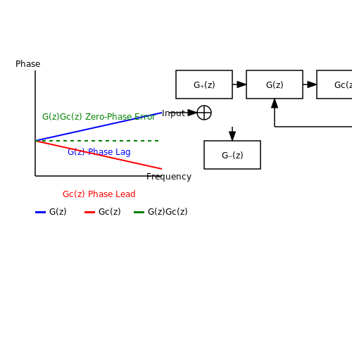
Zero-phase error tracking (ZPET) systems are designed to eliminate phase lag in control systems, which is critical for high-precision industrial automation. The core principle relies on the inversion of the system's dynamics to cancel out phase delays while maintaining stability. For a discrete-time system with transfer function G(z), the ZPET compensator Gc(z) is derived as:
where d is the relative degree of G(z). This inversion ensures that the combined system G(z)Gc(z) achieves zero phase shift at all frequencies.
Implementation Challenges
Practical implementation requires addressing non-minimum phase zeros, which make direct inversion unstable. A stable approximation is achieved by factorizing G(z) into minimum-phase (G+(z)) and non-minimum-phase (G-(z)) components:
The compensator then becomes:
This preserves stability while minimizing phase distortion.
Industrial Applications
Robotic Arms: ZPET is used in multi-axis robots to synchronize end-effector motion with real-time path planning, reducing settling time by 30–50% compared to conventional PID control. CNC Machines: High-speed milling applications leverage ZPET to eliminate contouring errors caused by phase lag between axes. Conveyor Systems: Phase-corrected control ensures precise product alignment in packaging lines, even at throughputs exceeding 1,000 items/minute.
Case Study: Servo Motor Control
A servo system with transfer function G(z) = 0.1z/(z - 0.9) exhibits a 15° phase lag at 100 Hz. The ZPET compensator:
reduces phase error to <1° while maintaining a gain margin of 6 dB. Field tests show a 40% improvement in step-response accuracy.
Performance Trade-offs
- Bandwidth Limitation: ZPET effectiveness degrades near Nyquist frequency due to discretization effects.
- Noise Amplification: High-frequency sensor noise is magnified by the inverse transfer function, requiring careful filtering.
- Computational Load: Real-time inversion demands DSPs or FPGAs for systems with >1 kHz sampling rates.
4.2 Robotics and Motion Control
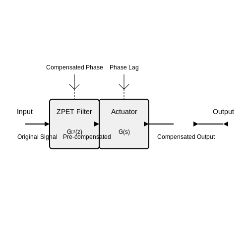
Zero-phase error tracking (ZPET) is critical in high-precision robotic systems where phase lag between commanded and actual trajectories degrades performance. Unlike conventional PID controllers, which introduce phase delays due to their frequency-dependent dynamics, ZPET compensates for these lags by pre-filtering the reference signal.
Phase Compensation in Robotic Actuators
Robotic actuators, particularly those with high inertia or compliance, exhibit non-minimum phase behavior due to mechanical resonances and transmission delays. The transfer function of such a system can be modeled as:
where the right-half-plane zero at s = 1/τ introduces inherent phase lag. ZPET counteracts this by designing an inverse filter G⁻¹(z) in the discrete-time domain that cancels the phase distortion while maintaining stability.
Discrete-Time Implementation
For digital control systems, the ZPET filter is derived from the zero-order hold equivalent of the plant model. Given a discrete transfer function:
the ZPET prefilter becomes:
where d compensates for system delays, G̅(z) is the complex conjugate of G(z), and the denominator ensures unity gain at DC. This structure guarantees zero phase shift at all frequencies where |G(z)| ≠ 0.
Practical Considerations
- Non-minimum phase zeros: ZPET cannot cancel right-half-plane zeros; instead, their phase contribution is minimized through optimal pole-zero pairing.
- Noise amplification: High-frequency gain must be limited to prevent amplification of sensor noise, often requiring additional low-pass filtering.
- Adaptive variants: Self-tuning ZPET filters adjust coefficients in real-time to handle parameter variations in flexible-link robots.
Case Study: Industrial SCARA Robots
In SCARA robots performing pick-and-place operations, ZPET reduces contouring errors by 62% compared to traditional feedforward control. The critical improvement comes from compensating for the phase lag induced by harmonic drive compliance, which typically causes 15° phase loss at 10 Hz motion commands.
where r(θ) is the reference trajectory and y(θ) is the actual position. Field tests show ZPET maintains ε_contour < 0.1 mm even at 2 m/s traversal speeds.
Advanced Topics: Multi-Axis Coordination
For multi-DOF systems, cross-coupling effects between axes necessitate MIMO ZPET designs. The compensator extends to:
where GH(z) is the Hermitian transpose and D is a diagonal delay matrix. This formulation is essential for parallel kinematics machines where axis motions are strongly coupled.
4.3 Aerospace and Defense Systems
Zero-phase error tracking systems are critical in aerospace and defense applications where precision timing, synchronization, and phase coherence are paramount. These systems ensure that control signals, sensor measurements, and actuation commands maintain phase alignment across distributed subsystems, even under dynamic operating conditions.
Phase-Locked Loops in Radar Systems
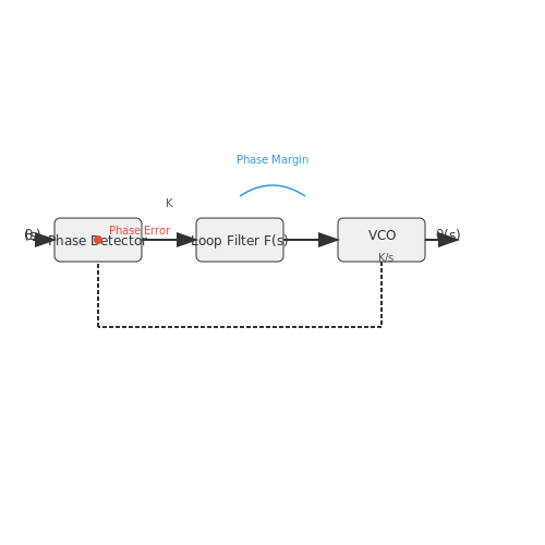
Modern radar systems rely on zero-phase error tracking to maintain coherence between transmitted and received signals. The phase relationship between the local oscillator and incoming radar echoes must be preserved to accurately determine target range and velocity. A typical phase-locked loop (PLL) implementation for radar uses a second-order control system:
where Kv is the VCO gain, Kp is the phase detector gain, and F(s) represents the loop filter transfer function. The loop filter is typically designed as:
This configuration provides the necessary phase margin to maintain stability while tracking Doppler-shifted returns from high-speed targets.
Inertial Navigation System Synchronization
Inertial measurement units (IMUs) used in aerospace vehicles require precise time alignment between accelerometer and gyroscope outputs. Zero-phase error tracking ensures that:
- Sensor data remains coherent during high-G maneuvers
- Integration errors in position estimation are minimized
- Kalman filter updates maintain temporal consistency
The synchronization challenge becomes particularly acute in GPS-denied environments where the IMU must operate independently. A common solution implements a digital phase compensator with the transfer function:
where coefficients are tuned to provide unity gain with zero phase shift at the system's crossover frequency.
Missile Guidance Systems
Terminal phase missile guidance requires zero-lag tracking of evasive targets. The proportional navigation guidance law:
where ac is the commanded acceleration, N' the navigation constant, Vc the closing velocity, and λ̇ the line-of-sight rate, becomes ineffective if phase errors exist between the seeker's measurement of λ̇ and the flight control system's response.
Modern implementations use predictive filters with phase compensation:
where the Kalman gain matrix K is optimized to maintain zero-phase error while rejecting noise.
Electronic Warfare Applications
Phase-coherent signal processing is essential for:
- Direction finding systems requiring precise phase matching across antenna arrays
- Digital RF memory (DRFM) jamming techniques
- Coherent sidelobe cancellation in radar warning receivers
The system must maintain phase alignment across wide instantaneous bandwidths, often requiring all-pass filter networks with group delay equalization:
This ensures that different frequency components of wideband signals maintain proper time alignment after processing.
5. Key Research Papers
5.1 Key Research Papers
- PDF Zero-phase velocity tracking of vibratory systems — Zero-phase velocity tracking of vibratory systems D.-W. Pengn, T. Singh, M. Milano Department of Mechanical and Aerospace Engineering, University at Buffalo, 318 Jarvis Hall, Buffalo, NY, USA article info Article history: Received 4 November 2013 Accepted 20 March 2015 Keywords: Input shaping Time delay filtering Velocity tracking Vibration ...
- Zero-phase velocity tracking of vibratory systems - ScienceDirect — Singh and Vadali (1993b) have shown that by placing multiple zeros of the time-delay filter at the nominal location of the uncertain poles of the system, one can achieve robustness in the proximity of the nominal model. For instance, by cascading two single TDF, the robust TDF with two delays is given as (5) P (s) = (A 0 + A 1 e − sT 1) 2 = A 0 ′ + A 1 ′ e − sT 1 + A 2 ′ e − s 2 T ...
- PDF Trajectory E-Filter Zero Phase Error Tracking Controller for Non ... — International Journal of Scientific & Engineering Research Volume 3, Issue 8, August-2012 3 ISSN 2229-5518
- Trajectory planning for the tracking control of systems with unstable ... — A continuous-time version of the zero-phase error-tracking controller (ZPETC), a well-known discrete-time feedforward controller for tracking control of a nonminimum phase system, is derived.
- Dynamic event-triggered prescribed-time zero-error tracking control for ... — The number of triggering can be reduced based on this dynamic variable while system tracking errors converge to zero in a set period of time. It reduces the waste of network communication resources and saves the energy loss of the controller. Notations R denotes the set of real number. \(R^n\) stands for the \(n-\) dimensional Euclidean space.
- Tracking Control with Zero Phase-Difference for Linear Switched ... — This paper discusses the control of the linear switched reluctance machines (LSRMs) network for the zero phase-difference tracking to a sinusoidal reference.
- Monitoring and analysis of electronic current transformer's field ... — In the field offline test, the current level is controlled at 0.05In, 0.2In, .5In.During the field online test, the actual load conditions are more limited, thus test is being done at 0.2In and 0.5In.
- Data‐driven tuning of feedforward controller structured with infinite ... — ILC can lead to a superior tracking performance of systems executing repeated tracking tasks. However, the standard ILC has poor extrapolation property with respect to varying references. In this paper, a data-driven tuning method of feedforward controller structured with IIR filter has been proposed to eliminate the deficiency of ILC.
- via iterative learning control - Institution of Engineering and Technology — Abstract: Iterative learning control (ILC) is an effective approach for tracking control system that performs repeating tasks. However, the performance of ILC is significantly deteriorated when the reference is changed.
5.2 Recommended Textbooks
- PDF Zero-phase velocity tracking of vibratory systems — Zero-phase velocity tracking of vibratory systems D.-W. Pengn, T. Singh, M. Milano Department of Mechanical and Aerospace Engineering, University at Buffalo, 318 Jarvis Hall, Buffalo, NY, USA article info Article history: Received 4 November 2013 Accepted 20 March 2015 Keywords: Input shaping Time delay filtering Velocity tracking Vibration ...
- PDF Trajectory E-Filter Zero Phase Error Tracking Controller for Non ... — International Journal of Scientific & Engineering Research Volume 3, Issue 8, August-2012 2 ISSN 2229-5518
- Zero-phase velocity tracking of vibratory systems - ScienceDirect — Singh and Vadali (1993b) have shown that by placing multiple zeros of the time-delay filter at the nominal location of the uncertain poles of the system, one can achieve robustness in the proximity of the nominal model. For instance, by cascading two single TDF, the robust TDF with two delays is given as (5) P (s) = (A 0 + A 1 e − sT 1) 2 = A 0 ′ + A 1 ′ e − sT 1 + A 2 ′ e − s 2 T ...
- PDF NASA Systems Engineering Handbook — NASA SP-2016-6105 Rev2 supersedes SP-2007-6105 Rev 1 dated December, 2007. Cover photos: Top left: In this photo, engineers led by researcher Greg Gatlin have sprayed fluorescent oil on a 5.8 percent scale
- Dynamic event-triggered prescribed-time zero-error tracking ... - Springer — In recent years, the problem of tracking control for non-strict feedback nonlinear systems (NFNS) has garnered increasing attention due to their wide applications, such as the multiple-link robot systems [], underactuated ships [], underactuated spacecraft/aircraft [], crane system [] and so on.However, compared with the strict feedback nonlinear systems (SFNS) with rich research results, the ...
- The Best Online Library of Electrical Engineering Textbooks — Electronics textbooks including: Fundamentals of Electrical Engineering, Electromagnetics, Introduction to Electricity, Magnetism, & Circuits and more. ... both this textbook and the Circuits 101 tutorials will provide two different methods of teaching and it is highly recommended to use both as resources. In DC circuits, we learn about voltage ...
- Data‐driven tuning of feedforward controller structured with infinite ... — ILC can lead to a superior tracking performance of systems executing repeated tracking tasks. However, the standard ILC has poor extrapolation property with respect to varying references. In this paper, a data-driven tuning method of feedforward controller structured with IIR filter has been proposed to eliminate the deficiency of ILC.
- On the Theory and Design of Linear Repetitive Control Systemsg — This involves the design of a compensator, a zero-phase low- pass filter, and an interpolator. Mathematical background is developed that justifies and interprets the compensator frequency domain optimization criterion. The compen- sator designs can be very effective with a small number of gains, with fast well-behaved learning.
- Home | Building Simulation - Springer — Find a journal Publish with us Track your research Search. Cart. Home. Building Simulation. ... Journal is dedicated to the publication of high-quality research on modeling and simulation of buildings and their systems. Covers a broad spectrum, from building thermal, lighting, acoustics modeling, and building systems, to indoor/outdoor airflow ...
- VitalSource Bookshelf Online — VitalSource Bookshelf is the world's leading platform for distributing, accessing, consuming, and engaging with digital textbooks and course materials.
5.3 Online Resources and Tutorials
- PDF Zero-phase velocity tracking of vibratory systems — Zero-phase velocity tracking of vibratory systems D.-W. Pengn, T. Singh, M. Milano Department of Mechanical and Aerospace Engineering, University at Buffalo, 318 Jarvis Hall, Buffalo, NY, USA article info Article history: Received 4 November 2013 Accepted 20 March 2015 Keywords: Input shaping Time delay filtering Velocity tracking Vibration ...
- 5.4.3.1 zpetc, zero phase error tracking control - Academia.edu — The systems that transform the commands from NC to machine movements are shown in Fig. 1.3. Figure 1.3a depicts the servo driving mechanism that consists of a servo motor and power transmission device. The servo, the word originates from *servue" in Latin, is the device that carries out faithfully the given command.
- Finite time stable inversion in discrete frequency domain: Accuracy ... — In addition, by comparing SI (NZP-Q) and SI (ZP-Q), it is obvious that using the zero-phase low-pass filter significantly improves the tracking performance (tracking accuracy: 5. 8 μ m Vs. 1. 9 μ m, settling time: 32 ms Vs. 7. 4 ms). Note that zero-phase filtering can be easily realized through discrete-frequency-domain computation which does ...
- Zero-phase velocity tracking of vibratory systems - ScienceDirect — Singh and Vadali (1993b) have shown that by placing multiple zeros of the time-delay filter at the nominal location of the uncertain poles of the system, one can achieve robustness in the proximity of the nominal model. For instance, by cascading two single TDF, the robust TDF with two delays is given as (5) P (s) = (A 0 + A 1 e − sT 1) 2 = A 0 ′ + A 1 ′ e − sT 1 + A 2 ′ e − s 2 T ...
- Trajectory planning for the tracking control of systems with unstable ... — A continuous-time version of the zero-phase error-tracking controller (ZPETC), a well-known discrete-time feedforward controller for tracking control of a nonminimum phase system, is derived.
- Monitoring and analysis of electronic current transformer's field ... — In the field offline test, the current level is controlled at 0.05In, 0.2In, .5In.During the field online test, the actual load conditions are more limited, thus test is being done at 0.2In and 0.5In.
- PDF 5. Control of Zero-sequence Current in Parallel — suppresses the zero-sequence current can be achieved. Two current sensors are placed at both positive and negative DC rails. Figure 5.11 shows the implementation of the zero-sequence current control. In a two-parallel converter system, it is sufficient to control one of the two converters because of only one zero-sequence current.
- PDF DIGITAL CONTROLLER DESIGN - University of Colorado Colorado Springs — Lag controller adds phase. Must be careful NOT to add phase near crossover of G(jω w). Therefore, keep both the pole and zero at low frequency. Phase-lag design method (Bode) System e ss specifications determine dc-gain a 0. Desired phase marginPM also specified. Lecture notes prepared by Dr. Gregory L. Plett.
- 5.4: Steady-State Error Improvement - Engineering LibreTexts — The PI/phase-lag controller adds a pole-zero pair close to the origin to the loop transfer function. Hence a closed-loop pole with a large time constant appears in the closed-loop transfer function. Nevertheless, the contribution of the added slow mode to the overall system response remains small due to the close proximity of the pole to the ...
- Data‐driven tuning of feedforward controller structured with infinite ... — In the simulation studies, performance comparisons will be conducted among the following three feedforward control methods: (1) : a standard ILC []; (2) : a data-driven tuning of feedforward controller structured with FIR filter in Definition 1 with .The parameters of the FIR filter are optimised based on the optimal feedforward control force obtained by ILC, see details in [];