Linear Variable Differential Transformers (LVDTs)
1. Definition and Basic Principle of Operation
1.1 Definition and Basic Principle of Operation
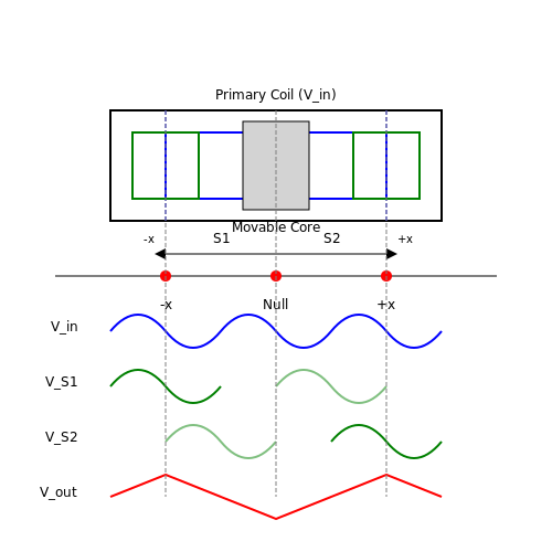
A Linear Variable Differential Transformer (LVDT) is an electromechanical transducer that converts linear displacement into a proportional electrical signal. It operates on the principle of mutual inductance between a primary winding and two symmetrically placed secondary windings, coupled via a movable ferromagnetic core. The output voltage varies differentially with core position, providing high accuracy, repeatability, and infinite resolution.
Core Components and Structure
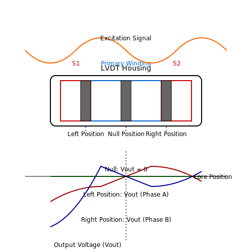
An LVDT consists of:
- Primary Winding: Energized by an AC excitation signal (typically 1–10 kHz).
- Secondary Windings (S1, S2): Wound symmetrically on either side of the primary, connected in series opposition.
- Ferromagnetic Core: Moves linearly within the bore, modulating magnetic coupling.
- Non-magnetic Housing: Provides mechanical stability and shields against external fields.
Operating Principle
When the core is centered (null position), voltages induced in S1 and S2 are equal but 180° out of phase, resulting in zero net output:
Displacing the core unbalances the mutual inductance, causing one secondary voltage to dominate. The output voltage magnitude is proportional to displacement, while its phase indicates direction:
where K is a sensitivity constant (V/V/mm), x is displacement, and Vpri is the primary excitation voltage.
Phase-Sensitive Demodulation
LVDT outputs require synchronous demodulation to resolve directionality. A phase-sensitive detector (PSD) compares the output phase to the excitation signal:
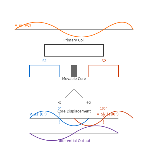
- 0° phase difference: Core displacement toward S1.
- 180° phase difference: Core displacement toward S2.
Advantages Over Potentiometric Sensors
LVDTs exhibit:
- Frictionless operation: No contact between core and windings eliminates wear.
- High linearity: ±0.25% full-scale deviation is typical.
- Environmental robustness: Immune to dust, humidity, and temperature variations.
Core Components and Their Functions
Primary Winding
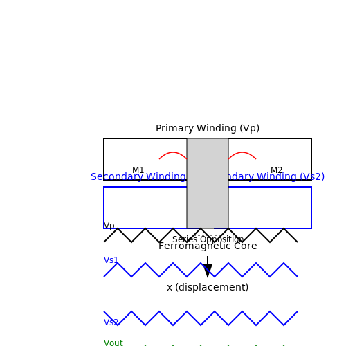
The primary winding is an inductive coil excited by an alternating current (AC) source, typically in the range of 1–10 kHz. When energized, it generates a time-varying magnetic field that couples with the secondary windings via the movable core. The excitation voltage Vp is given by:
where Vrms is the root-mean-square voltage and ω is the angular frequency. The primary winding's inductance Lp depends on core position, influencing the mutual inductance with the secondaries.
Secondary Windings
Two identical secondary windings, wound in series opposition, are positioned symmetrically around the primary. The induced voltages Vs1 and Vs2 are:
where M1 and M2 are mutual inductances between the primary and each secondary. The differential output Vout is:
where k is a sensitivity constant and x is core displacement.
Movable Core
The ferromagnetic core, typically made of nickel-iron alloy, modulates the magnetic coupling between windings. Its position determines the voltage imbalance in the secondaries. Core movement is mechanically linked to the measured displacement, with linearity errors below 0.1% in precision LVDTs.
Signal Conditioning Electronics
Modern LVDTs integrate demodulation circuits to convert the AC output to a DC signal proportional to displacement. A synchronous demodulator eliminates phase-sensitive errors by multiplying the output with a reference signal:
where T is the excitation period.
Mechanical Housing
The housing provides structural integrity and shields the windings from electromagnetic interference. Materials like stainless steel or anodized aluminum are chosen for thermal stability in industrial environments.
Connectors and Cabling
Shielded twisted-pair cables minimize noise pickup in the low-millivolt output signal. High-quality connectors ensure reliable contact resistance below 10 mΩ, critical for long-term stability in aerospace and automotive applications.
1.3 Electromagnetic Induction in LVDTs
Fundamental Principle of Induction
The operation of a Linear Variable Differential Transformer (LVDT) relies on Faraday's Law of Electromagnetic Induction, which states that a changing magnetic flux through a conductor induces an electromotive force (EMF). For an LVDT, this principle is applied via a primary coil excited by an alternating current (AC) and two secondary coils wound in opposition. The core's position modulates the mutual inductance between the primary and secondary coils, generating a differential voltage output.
Here, N is the number of turns in the secondary coil, and dΦB/dt is the time rate of change of magnetic flux. The negative sign indicates Lenz's Law, which ensures the induced EMF opposes the change in flux.
Mutual Inductance and Core Displacement
The coupling between the primary and secondary coils is described by mutual inductance M, which varies linearly with core position x. When the core is centered, the induced voltages in the two secondary coils are equal and cancel out. Displacing the core unbalances the mutual inductance, producing a net differential voltage:
where k is a sensitivity constant, Vin is the excitation voltage, and ω is the angular frequency. The output voltage's amplitude is proportional to displacement, while its phase indicates direction.
Phase-Sensitive Demodulation
LVDTs often employ phase-sensitive detectors to resolve the direction of displacement. The secondary voltage's phase shifts by 180° depending on whether the core moves left or right of center. A synchronous demodulator compares the output phase to the excitation signal, converting the AC output into a DC signal whose polarity reflects displacement direction.
Practical Design Considerations
- Excitation Frequency: Higher frequencies (1–10 kHz) improve sensitivity but increase eddy current losses.
- Core Material: High-permeability alloys like Mu-metal minimize hysteresis and enhance linearity.
- Shielding: Electromagnetic shielding reduces noise interference in industrial environments.
Mathematical Derivation of Output Voltage
The induced voltage in each secondary coil is derived from the mutual inductance M1 and M2, which vary with core position x:
Assuming linear coupling variation, M1 = M0 + ΔM and M2 = M0 - ΔM, where ΔM ∝ x. The differential output becomes:
Substituting Ip = Vin/(jωLp) for the primary current, where Lp is the primary inductance, yields:
This confirms the linear relationship between Vout and displacement x.
2. Primary and Secondary Coils Configuration
2.1 Primary and Secondary Coils Configuration
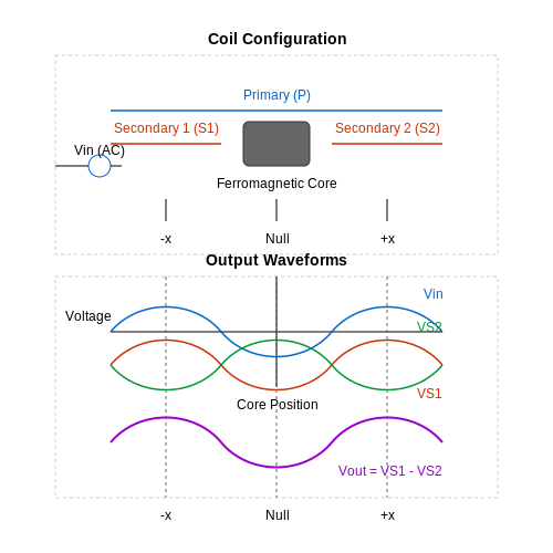
The core of an LVDT's operation lies in its electromagnetic coupling between the primary and secondary coils. The primary coil is excited by an alternating current (AC) source, typically in the range of 1–10 kHz, generating a time-varying magnetic field. This field induces voltages in the two secondary coils, which are wound symmetrically on either side of the primary coil.
Electromagnetic Coupling and Phase Relationships
The secondary coils are connected in series opposition, meaning their induced voltages subtract rather than add. When the ferromagnetic core is centered (null position), the voltages induced in the secondary coils are equal in magnitude but opposite in phase, resulting in a net output of zero. Displacement of the core unbalances the mutual inductance between the primary and secondary coils, producing a differential voltage proportional to the core's position.
Here, k is a sensitivity constant dependent on coil geometry and excitation frequency, x is the core displacement, and Vin is the primary excitation voltage. The phase of Vout reverses when the core crosses the null position, providing directional information.
Coil Winding Techniques
Precision winding is critical to minimize nonlinearities and temperature drift. Key design considerations include:
- Symmetry: Secondary coils must have identical turns and winding density to ensure balanced outputs at null.
- Layer stacking: Primary windings are often sandwiched between secondary layers to enhance coupling uniformity.
- Wire selection: High-temperature enameled copper wire is standard, with polyimide insulation for extreme environments.
Modern LVDTs often use computerized winding machines to achieve tolerances better than ±0.1% in turn count matching.
Frequency-Dependent Behavior
The excitation frequency affects both sensitivity and phase response. The optimal frequency balances three factors:
where Lp is primary inductance and Cp is parasitic capacitance. Higher frequencies improve sensitivity but increase eddy current losses in the core, while lower frequencies reduce resolution due to decreased inductive coupling.
Practical Implementation Challenges
In aerospace and nuclear applications, radiation-hardened designs employ:
- Bifilar winding to cancel magnetic pickup noise
- Potting compounds with low outgassing properties
- Molybdenum core materials for high-temperature stability
Calibration procedures typically involve laser-measured displacement stages to characterize nonlinearity, which remains below 0.25% of full-scale in precision LVDTs.
2.2 Core Materials and Their Impact on Performance
The performance of a Linear Variable Differential Transformer (LVDT) is heavily influenced by the material properties of its movable core. The core's permeability, hysteresis, and eddy current losses directly affect sensitivity, linearity, and frequency response. Optimal core selection balances magnetic efficiency with mechanical durability.
Magnetic Permeability and Core Saturation
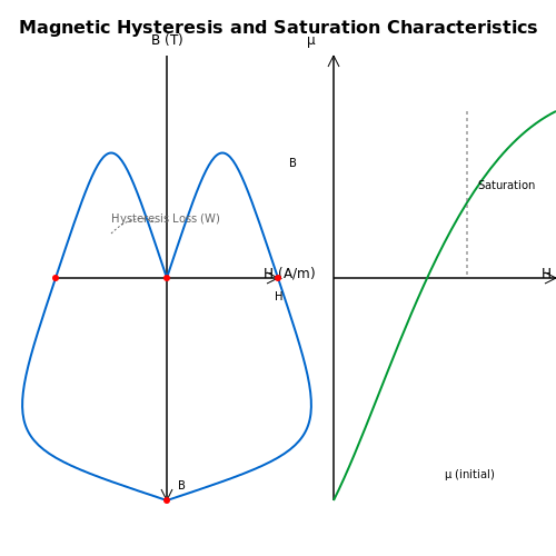
The relative permeability (μr) of the core material determines how effectively it concentrates magnetic flux, directly influencing the LVDT's sensitivity. High-permeability materials such as permalloy (78-80% nickel-iron) or supermalloy (79% nickel, 15% iron, 5% molybdenum) enhance signal output by reducing reluctance in the magnetic circuit. However, these materials exhibit saturation effects at high excitation currents, governed by:
where Bsat is the saturation flux density, μ0 is the permeability of free space, and H is the magnetic field intensity. Exceeding Bsat introduces nonlinearity, degrading measurement accuracy.
Hysteresis and Temperature Stability
Core materials with low coercivity (Hc) minimize hysteresis losses, ensuring repeatability in cyclic measurements. Annealed Mu-metal (77% nickel, 16% iron, 5% copper, 2% chromium) is a common choice for precision LVDTs due to its near-zero hysteresis and temperature stability. The hysteresis loop area represents energy loss per cycle:
Temperature coefficients of permeability must also be considered; for instance, nickel-iron alloys exhibit a μr variation of ~0.2%/°C, necessitating compensation in high-precision applications.
Eddy Current Losses and Frequency Response
Laminated or powdered cores mitigate eddy currents, which become significant at excitation frequencies above 1 kHz. The eddy current power loss (Pe) in a solid core is approximated by:
where f is frequency, B is peak flux density, t is material thickness, and ρ is resistivity. Powdered ferrite cores (e.g., Mn-Zn or Ni-Zn) are preferred for high-frequency LVDTs (>10 kHz) due to their inherent resistivity and minimal skin effect.
Mechanical Considerations
Core materials must withstand mechanical stress without magnetic degradation. Martensitic stainless steels (e.g., 17-4PH) are used in harsh environments, though their lower permeability reduces sensitivity. For non-magnetic housings, Inconel or titanium provide corrosion resistance while minimizing magnetic interference.
Practical Trade-offs in Material Selection
- High Sensitivity: Permalloy or supermalloy cores (high μr, low Hc).
- High Frequency: Ferrite or laminated silicon steel (low Pe).
- Harsh Environments: Stainless steel or Inconel (mechanical robustness).
2.3 Mechanical Structure and Housing
Core Components and Material Selection
The mechanical integrity of an LVDT relies on its housing, which typically consists of a non-magnetic stainless steel or aluminum alloy casing. The primary winding and secondary coils are wound on a thermally stable bobbin, often made of glass-reinforced polymer or ceramic to minimize thermal expansion effects. The core, usually constructed from nickel-iron alloy or ferrite, slides within a precision-ground bore with tolerances as tight as ±5 µm to ensure consistent magnetic coupling.
Housing Design Considerations
LVDT housings must provide:
- Hermetic sealing for operation in harsh environments (IP67 or higher)
- Low thermal expansion coefficients (α < 11 × 10-6/°C for matched materials)
- Vibration resistance with natural frequencies > 500 Hz to avoid resonance
The housing's axial stiffness k can be derived from the Young's modulus E and geometry:
where A is the cross-sectional area and L is the effective length of the housing structure.
Bearing Systems and Friction Management
High-performance LVDTs employ:
- Precision ball bearings with preload adjustments (typical friction < 0.1 N)
- Air bearings in metrology-grade units (friction < 0.001 N)
- Self-lubricating polymer bushings for cost-sensitive applications
The Stribeck curve governs friction behavior:
where Fc is Coulomb friction, Fs is static friction, v is velocity, and vs is the Stribeck velocity.
Environmental Protection Methods
Advanced sealing techniques include:
- Welded metal bellows for ultra-high vacuum applications
- Multi-stage labyrinth seals with hydrophobic coatings
- Inert gas purging (typically nitrogen or argon) for corrosive environments
The permeation rate Q through seals follows:
where P is permeability, A is area, Δp is pressure differential, and d is seal thickness.
Mounting and Mechanical Interfaces
Standard mounting configurations include:
- Flange mounts with DIN 3-hole or 4-hole patterns
- Threaded stud mounts (typically M3 to M12)
- Dovetail rails for optical table integration
Mounting-induced error εm due to angular misalignment θ is:
where L is the probe length and θ is in radians.
3. Phase-Sensitive Demodulation Techniques
3.1 Phase-Sensitive Demodulation Techniques
Phase-sensitive demodulation (PSD) is essential for extracting displacement information from an LVDT's output signal, which is typically amplitude-modulated (AM) by the core position. The technique resolves both the magnitude and direction of displacement by leveraging the phase relationship between the primary excitation signal and the secondary output.
Principle of Operation
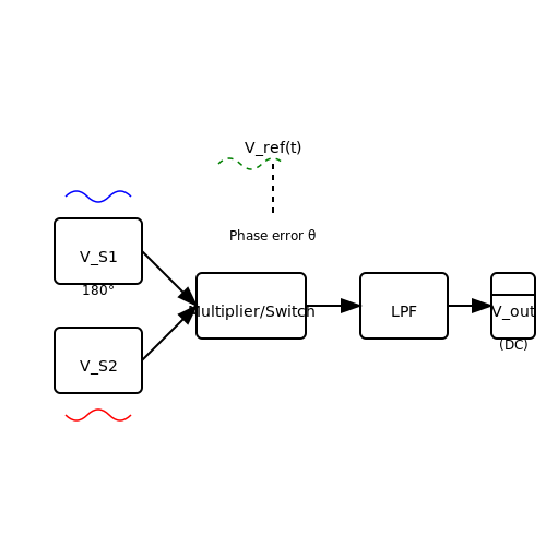
The secondary voltages of an LVDT, VS1 and VS2, are 180° out of phase when the core is displaced from null. A phase-sensitive demodulator multiplies the secondary signal by a reference signal synchronous with the primary excitation, then applies low-pass filtering to extract the DC component proportional to displacement:
where Vsec(t) is the secondary voltage, Vref(t) is the reference signal, and T is the excitation period. The result is a signed DC voltage whose polarity indicates displacement direction.
Implementation Methods
Analog Multiplier Approach
Analog multipliers (e.g., Gilbert cell) directly multiply the secondary signal by a square-wave or sinusoidal reference. The output is filtered to reject high-frequency components:
where K is the multiplier gain, Asec and Aref are amplitudes, and φ is the phase difference. A zero-phase shift ensures maximum sensitivity.
Switched Demodulator
Cost-effective implementations use synchronous switches to invert the secondary signal polarity at the excitation frequency. The switching action is equivalent to multiplication by a ±1 square wave:
Followed by an RC low-pass filter with cutoff << fexcitation, this extracts the displacement-proportional DC component.
Phase Alignment Considerations
Optimal performance requires precise phase matching between reference and secondary signals. A phase error θ introduces gain error proportional to cos(θ):
Practical systems use phase-locked loops (PLLs) or adjustable delay lines to minimize this error. Modern digital implementations achieve sub-degree phase accuracy through real-time correlation algorithms.
Digital PSD Techniques
Digital signal processors (DSPs) implement PSD via synchronous sampling and numerical integration. The secondary signal is sampled at multiple points per cycle, then multiplied by a digital reference:
where N is samples per cycle. This method inherently rejects harmonics and provides programmable phase adjustment.
3.2 Output Voltage Characteristics
The output voltage of an LVDT is a function of the core displacement and exhibits a well-defined linear relationship within its operational range. The voltage differential between the two secondary windings, V1 and V2, is processed to determine the magnitude and direction of core movement.
Mathematical Derivation of Output Voltage
The induced voltages in the secondary windings are proportional to the mutual inductance between the primary and each secondary coil. Assuming sinusoidal excitation Vp = V0 sin(ωt), the output voltages can be expressed as:
where k1 and k2 are coupling coefficients dependent on the core position, and x is the displacement from the null point. The differential output voltage Vout is:
For a symmetrically wound LVDT, the coupling coefficients vary linearly with displacement, yielding:
where K is the sensitivity factor (typically in mV/V/mm).
Phase-Sensitive Demodulation
Since the output is an amplitude-modulated signal, phase-sensitive demodulation is employed to recover the displacement polarity. A reference signal synchronous with the primary excitation is used to distinguish in-phase (positive displacement) and out-of-phase (negative displacement) components.
Nonlinearity and Sensitivity
While LVDTs exhibit high linearity (±0.25% full-scale typical) within the specified range, nonlinearities arise at displacement extremes due to magnetic saturation and fringing effects. Sensitivity is influenced by:
- Excitation frequency: Typically 1-10 kHz, with higher frequencies reducing eddy current losses.
- Core material: High-permeability nickel-iron alloys optimize flux linkage.
- Temperature effects: Compensated through ratiometric measurement (Vout/Vexcitation).
Practical Measurement Considerations
In industrial applications, the output is often conditioned using instrumentation amplifiers with:
- High common-mode rejection ratio (CMRR > 80 dB)
- Programmable gain to match the ADC input range
- Built-in demodulation for DC output conversion
Modern signal conditioning ICs (e.g., AD598, NE5521) integrate these functions, providing temperature-stabilized outputs with 16-bit resolution.
3.3 Null Position and Linearity
Null Position in LVDTs
The null position of an LVDT is the core displacement where the differential output voltage (Vout) becomes zero. At this point, the induced voltages in the secondary windings (S1 and S2) are equal in magnitude but opposite in phase, resulting in perfect cancellation. Mathematically:
The null position is typically the mechanical center of the LVDT’s stroke range. Deviations from this position introduce a phase-sensitive output voltage proportional to displacement. In high-precision applications, minimizing null voltage (residual voltage at null) is critical, as it can arise from asymmetries in winding geometry or magnetic imbalances.
Linearity and Its Practical Implications
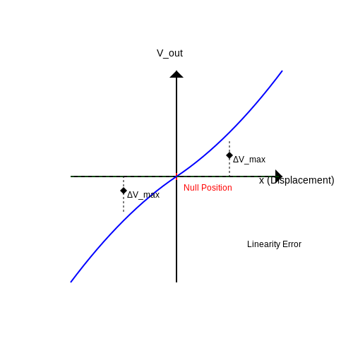
LVDTs exhibit a linear relationship between core displacement and output voltage within a specified range. The linearity error quantifies the deviation from this ideal behavior, often expressed as a percentage of full-scale output. For a displacement x, the output voltage is:
where K is the sensitivity constant, and ε(x) represents nonlinearity. Key factors affecting linearity include:
- Magnetic flux distribution: Nonuniform coupling between primary and secondary windings.
- Core material and geometry: Saturation effects or edge discontinuities.
- Electromagnetic interference: Stray fields distorting the output signal.
Quantifying Linearity Error
Linearity is often characterized using the best-fit straight line method. The maximum deviation (ΔVmax) from this line, relative to full-scale output (VFS), defines the error:
Advanced LVDTs achieve linearity errors below ±0.25% of full scale. Calibration techniques, such as lookup tables or polynomial correction, further enhance accuracy in precision systems like aerospace actuators or metrology tools.
Phase-Sensitive Demodulation and Null Stability
The output voltage’s phase (0° or 180° relative to the excitation) indicates displacement direction. At the null position, a 90° phase shift occurs, which is exploited in phase-sensitive demodulators to reject quadrature noise. Temperature drift and excitation voltage stability directly impact null repeatability, necessitating stable AC signal conditioning.
4. Industrial Displacement Measurement
4.1 Industrial Displacement Measurement
Linear Variable Differential Transformers (LVDTs) are widely employed in industrial settings for high-precision displacement measurement due to their robustness, linearity, and contactless operation. Their working principle relies on electromagnetic induction, where a movable ferromagnetic core alters the mutual inductance between primary and secondary coils, producing a differential voltage output proportional to displacement.
Operating Principle and Signal Conditioning
The LVDT consists of a primary coil excited by an AC carrier signal (typically 1–10 kHz) and two symmetrically wound secondary coils connected in series opposition. When the core is centered (null position), the induced voltages in the secondary coils cancel out, yielding zero net output. Displacement of the core unbalances the mutual inductance, generating a differential voltage:
where k is a sensitivity constant, x is the core displacement, and Vin is the excitation voltage. The output voltage's phase indicates displacement direction (0° or 180° relative to the carrier).
Demodulation and Linearization
To extract the displacement signal, synchronous demodulation is employed. A phase-sensitive detector (PSD) multiplies the LVDT output by a reference signal synchronous with the carrier, followed by low-pass filtering to recover the DC component:
where φ is the phase difference between the carrier and output. Non-linearity at extreme displacements is minimized through coil design and calibration, achieving typical linearity errors below ±0.25% of full-scale range.
Industrial Applications and Case Studies
LVDTs are favored in harsh environments due to their immunity to dust, moisture, and temperature variations. Key applications include:
- Hydraulic cylinder positioning in manufacturing automation, where sub-micron resolution is required.
- Vibration monitoring in turbines and rotating machinery, leveraging their high bandwidth (up to 1 kHz).
- Material testing machines, where their infinite resolution ensures accurate strain measurement.
A case study in aerospace involves using LVDTs for actuator feedback in flight control systems, where their failure-proof design meets DO-178C safety standards. Redundant LVDT configurations are often employed to ensure reliability.
Performance Trade-offs and Calibration
While LVDTs offer superior repeatability (±0.01% of full scale), their accuracy depends on:
- Excitation voltage stability (< 0.1% drift).
- Temperature compensation (active or passive).
- Mechanical alignment of the core to prevent off-axis errors.
Calibration involves a traceable reference standard (e.g., laser interferometer) to map voltage-to-displacement. Modern digital signal processors (DSPs) enable real-time linearization and temperature correction through polynomial fitting.
Comparison with Alternative Technologies
LVDTs outperform potentiometers (wear-prone) and capacitive sensors (sensitive to contamination) in industrial environments. However, magnetostrictive sensors may be preferred for very long strokes (> 1 m), while optical encoders excel in ultra-high-resolution applications.
4.2 Aerospace and Automotive Applications
High-Reliability Position Sensing in Aerospace
Linear Variable Differential Transformers (LVDTs) are extensively used in aerospace due to their robustness, high accuracy, and immunity to electromagnetic interference. Their contactless operation eliminates mechanical wear, making them ideal for flight control systems, such as:
- Thrust vector control in rocket engines, where precise nozzle positioning is critical.
- Flap and slat position monitoring in aircraft wings, ensuring aerodynamic efficiency.
- Landing gear deployment sensors, where failure tolerance is non-negotiable.
The LVDT's output voltage Vout is linearly proportional to the displacement x of the core:
where k is the sensitivity constant (typically 0.1–10 mV/V/mm). Aerospace-grade LVDTs operate at frequencies >1 kHz to avoid interference from avionics systems.
Automotive Safety and Performance Systems
In automotive engineering, LVDTs provide sub-millimeter resolution for:
- Suspension travel measurement in active damping systems, enabling real-time adjustments.
- Brake pedal position sensing for anti-lock braking systems (ABS), where response time <1 ms is critical.
- Transmission shift fork positioning in dual-clutch systems, reducing gear engagement errors.
Case Study: Steer-by-Wire Systems
Modern steer-by-wire architectures replace mechanical linkages with LVDTs to measure steering wheel angle. The sensor's differential output rejects common-mode noise from the vehicle's 12V/24V power system. A dual-redundant LVDT configuration is often employed, with the system comparing outputs:
Discrepancies beyond ±0.5% trigger fault detection algorithms. Automotive LVDTs must meet ISO 26262 ASIL-D standards for functional safety.
Environmental Tolerance Requirements
Both aerospace and automotive applications demand extreme environmental resilience:
| Parameter | Aerospace | Automotive |
|---|---|---|
| Temperature Range | -55°C to +125°C | -40°C to +150°C |
| Vibration Resistance | 50 g (10–2000 Hz) | 20 g (5–500 Hz) |
| IP Rating | IP67 (pressurized cabins) | IP69K (underhood) |
MIL-STD-810G and SAE J1211 govern the qualification testing for these conditions. The LVDT's hermetically sealed construction prevents moisture ingress, while nickel-iron cores maintain linearity across the temperature range.
5. Environmental and Operational Constraints
5.2 Environmental and Operational Constraints
Temperature Effects
LVDTs exhibit sensitivity to temperature variations due to thermal expansion of core and coil materials. The differential output voltage Vout is influenced by changes in the permeability (μ) of the core and the resistivity (ρ) of the windings. The temperature coefficient of resistance (TCR) for copper windings is approximately +0.393%/°C, leading to a measurable shift in the primary excitation current. For a typical LVDT with a nickel-iron core, the permeability-temperature relationship follows:
where μ0 is permeability at reference temperature T0, and α is the thermal coefficient of permeability (~−0.002/°C for Ni-Fe alloys). Compensating for this requires either temperature-stabilized excitation or algorithmic correction in the signal conditioning stage.
Vibration and Shock
Mechanical resonance frequencies of the LVDT structure must be considered in high-vibration environments. The natural frequency fn of the core-spring assembly is given by:
where k is the spring constant of the restoring mechanism and m is the core mass. Exceeding fn can induce harmonic distortion in the output. Industrial LVDTs often incorporate damping fluids or elastomeric mounts to attenuate vibrations above 100 Hz.
Electromagnetic Interference (EMI)
The low-level AC output (typically 1–50 mV/V) makes LVDTs susceptible to EMI. Twisted-pair cabling with grounded shields is mandatory for noise rejection. The common-mode rejection ratio (CMRR) of the signal conditioner should exceed 80 dB at the excitation frequency (usually 1–10 kHz). Faraday shielding of the coil assembly reduces capacitive coupling from nearby power lines.
Pressure and Humidity
Hermetically sealed LVDTs are required for operation in high-pressure (e.g., hydraulic systems) or high-humidity environments. Moisture ingress alters dielectric properties between windings, causing phase shifts in the output. Military-grade units (per MIL-PRF-39032) use glass-to-metal seals to maintain performance at 100% relative humidity.
Long-Term Stability
Core material aging affects hysteresis and linearity over time. Annealed Permalloy cores exhibit drift rates below 0.1%/year, while sintered ferrites may drift up to 0.5%/year. Calibration intervals should be adjusted accordingly for metrology-grade applications.
Power Supply Constraints
Excitation voltage stability directly impacts scale factor accuracy. A 1% variation in primary voltage induces a proportional error in Vout. Ratiometric measurement techniques eliminate this dependency by referencing the output to the input voltage:
Material Compatibility
In corrosive environments (e.g., chemical processing), housing materials must resist oxidation. 316L stainless steel or Inconel are preferred for wetted parts. Non-metallic variants with PEEK or ceramic housings are available for extreme conditions.
5.3 Comparison with Other Displacement Sensors
Linear Variable Differential Transformers (LVDTs) are widely used for high-precision displacement measurements, but their performance must be evaluated against alternative technologies such as potentiometers, capacitive sensors, and optical encoders. Each sensor type has distinct advantages and trade-offs in terms of resolution, linearity, environmental robustness, and cost.
Potentiometric Sensors
Potentiometers measure displacement through a sliding contact on a resistive element, providing a simple voltage-divider output. While inexpensive and easy to interface, they suffer from mechanical wear, limited resolution, and reduced lifespan due to friction. LVDTs, in contrast, are contactless, eliminating wear and enabling sub-micron resolution. The linearity of potentiometers typically ranges between 0.1% and 1%, whereas precision LVDTs achieve linearity better than 0.1% of full-scale range.
Capacitive Displacement Sensors
Capacitive sensors detect position changes by measuring variations in capacitance between parallel plates. They offer nanometer-scale resolution and high bandwidth but are sensitive to environmental factors such as humidity and dielectric changes. LVDTs are less affected by contaminants or temperature fluctuations due to their inductive operating principle. The output of a capacitive sensor follows:
where ϵ is the permittivity, A is the plate area, and d is the separation distance. Non-linearities arise from edge effects and stray capacitance, whereas LVDTs maintain linearity across their specified range.
Optical Encoders
Optical encoders use gratings or interferometry to achieve ultra-high resolution (often below 1 nm) but require clean environments and precise alignment. Incremental encoders lose position on power-off unless referenced, while absolute encoders are complex and costly. LVDTs provide absolute position measurement without requiring power-up initialization and are more tolerant of vibration and misalignment.
Strain-Gauge-Based Sensors
Strain gauges bonded to flexures measure displacement via resistance changes under deformation. They are compact and low-cost but exhibit hysteresis and creep under cyclic loading. LVDTs avoid these issues with frictionless operation and higher repeatability. Strain gauge output is temperature-sensitive, necessitating compensation circuits, whereas LVDTs inherently reject common-mode temperature effects.
Hall Effect Sensors
Hall effect sensors detect magnetic field changes from a moving target. While suitable for short-range applications, their non-linearity and sensitivity to external magnetic fields limit precision. LVDTs use shielded coils to minimize interference and provide a linear output proportional to core position, making them preferable for metrology-grade applications.
Piezoelectric Sensors
Piezoelectric devices generate charge under mechanical stress, enabling dynamic displacement measurement with high bandwidth. However, they cannot measure static positions due to charge leakage. LVDTs operate bidirectionally in both static and dynamic regimes, with frequency responses typically up to 1 kHz for standard models.
Summary of Key Metrics
| Sensor Type | Resolution | Linearity | Environmental Robustness | Lifespan |
|---|---|---|---|---|
| LVDT | 0.1 µm | 0.1–0.5% FS | High | >10⁷ cycles |
| Potentiometer | 10 µm | 0.5–1% FS | Moderate | 10⁵–10⁶ cycles |
| Capacitive | 1 nm | 0.01–0.1% FS | Low | High (no contact) |
| Optical Encoder | 1 nm | ±1 count | Low | High (no contact) |
6. Calibration Procedures and Standards
6.1 Calibration Procedures and Standards
Fundamentals of LVDT Calibration
Calibration of an LVDT ensures its output voltage accurately represents the displacement of the core. The relationship between displacement x and output voltage Vout is ideally linear, given by:
where S is the sensitivity (mV/V/mm) and Voffset is the null voltage at zero displacement. Calibration corrects deviations from this ideal behavior due to manufacturing tolerances, temperature effects, or aging.
Static Calibration Procedure
Static calibration involves applying known displacements and recording the corresponding output voltages. A high-precision micrometer stage or optical encoder provides reference displacement values. The steps are:
- Null Position Adjustment: Center the core and adjust the signal conditioner to zero the output.
- Full-Scale Calibration: Move the core to maximum positive and negative displacements, recording Vout at fixed intervals.
- Linearity Check: Verify that deviations from the best-fit line remain within the LVDT's specified linearity error (typically ±0.25% to ±0.5% of full scale).
Dynamic Calibration and Frequency Response
For applications involving rapid motion, dynamic calibration assesses the LVDT's frequency response. The transfer function H(f) is derived from:
where X(f) is the input displacement spectrum. A shaker table or piezoelectric actuator generates controlled sinusoidal displacements, while a spectrum analyzer captures Vout(f). The LVDT's bandwidth is the frequency at which the output amplitude drops by −3 dB.
Traceability and Standards Compliance
Calibration must adhere to metrology standards such as ISO/IEC 17025 or ASTM E2309. Key requirements include:
- Traceable Reference Standards: Displacement references (e.g., laser interferometers) must be NIST-traceable.
- Environmental Control: Temperature stability (±1°C) and vibration isolation to minimize measurement uncertainty.
- Uncertainty Budget: Document contributions from reference instruments, repeatability, and environmental factors.
Automated Calibration Systems
Modern systems use software-controlled stages and data acquisition to streamline calibration. A LabVIEW or Python script automates:
- Positioning the core via stepper motors.
- Recording Vout with a calibrated digital multimeter (DMM).
- Calculating sensitivity, linearity error, and hysteresis.
Practical Considerations
Field calibration may require portable equipment, such as handheld signal conditioners with built-in calibration routines. For harsh environments, in-situ verification using known mechanical stops or gauge blocks ensures continued accuracy without disassembling the LVDT.
6.2 Common Issues and Troubleshooting
Electrical Noise and Interference
LVDTs are susceptible to electromagnetic interference (EMI) and ground loops, which can introduce noise into the output signal. High-frequency noise often manifests as erratic fluctuations in the measured displacement. To mitigate this, use shielded twisted-pair cables for signal transmission and ensure proper grounding. The differential nature of LVDTs inherently rejects common-mode noise, but improper shielding can degrade this advantage.
where k is Boltzmann's constant, T is temperature, R is resistance, and Δf is bandwidth. For critical applications, employ active filtering with a cutoff frequency below the LVDT's excitation frequency.
Core Misalignment and Mechanical Binding
Mechanical misalignment between the core and bore can cause nonlinearity or complete signal dropout. Symptoms include abrupt changes in output voltage when the core reaches certain positions. Verify:
- Core concentricity within ±5% of bore diameter
- Absence of axial rotation during movement
- Proper clearance (typically 0.05-0.2 mm)
Binding often occurs due to contamination; periodic cleaning with isopropyl alcohol maintains smooth operation.
Excitation Voltage Instability
The LVDT's output scales directly with excitation voltage. A 1% variation in input voltage causes a 1% output error. Common issues include:
- Poorly regulated power supplies (ripple > 0.1%)
- Long cable runs causing voltage drop
- Thermal drift in oscillator circuits
For precision applications, use excitation voltages stabilized to ±0.01% with low-temperature-coefficient oscillators (e.g., crystal-based).
Phase Shift Errors
Ideal LVDTs produce in-phase (0°) or out-of-phase (180°) signals relative to excitation. Practical units exhibit phase shifts due to:
where ω is angular frequency, L is inductance, and R is winding resistance. Phase-sensitive demodulators must compensate for this shift to avoid amplitude errors. Modern signal conditioners auto-null phase errors during calibration.
Temperature Effects
Temperature changes affect both mechanical and electrical parameters:
| Parameter | Typical Temp Coefficient |
|---|---|
| Core permeability | 0.02%/°C |
| Winding resistance | 0.39%/°C (copper) |
| Bore diameter | 11 ppm/°C (stainless steel) |
For operation beyond ±10°C from calibration temperature, use temperature-compensated LVDTs or apply software corrections based on embedded RTD measurements.
Signal Conditioner Faults
Over 60% of LVDT system failures originate in signal conditioning electronics. Key failure modes include:
- Demodulator diode degradation (reverse leakage current > 1 μA)
- Op-amp offset drift exceeding specifications
- ADC reference voltage instability
Implement periodic self-tests by injecting known calibration signals through a multiplexer. Monitor power supply voltages and oscillator frequency as early failure indicators.
Residual Voltage
Even at null position, LVDTs output a small residual voltage (typically 0.1-1% of full scale) due to:
- Capacitive coupling between windings
- Minor core asymmetries
- Stray magnetic fields
Null voltage should remain stable over time. Sudden changes indicate winding shorts or core damage. High-end conditioners provide auto-nulling circuits that subtract residual voltage during zero calibration.
6.3 Long-Term Reliability and Durability
Mechanical Wear and Fatigue Resistance
The core mechanism of an LVDT relies on the frictionless movement of a ferromagnetic core within a bobbin assembly. Unlike potentiometric sensors, LVDTs exhibit minimal mechanical wear due to the absence of sliding electrical contacts. The primary wear mechanisms arise from:
- Core-guide interaction: Over extended cycles, the core may induce microscopic abrasion on the bore surface, particularly in high-frequency applications.
- Spring fatigue: Return springs in spring-centered LVDTs experience cyclic stress, governed by the modified Goodman relation:
where σa is the allowable stress amplitude, σ'f the fatigue strength coefficient, σm the mean stress, and σu the ultimate tensile strength. Advanced designs use beryllium-copper alloys for springs, achieving >107 cycles at full stroke.
Environmental Degradation Factors
LVDT housings typically employ 300-series stainless steel or anodized aluminum, providing IP67 or better protection. Key degradation modes include:
- Corrosion: Chloride-induced pitting in marine environments follows the empirical rate:
where D is pit depth, k the rate constant, CCl- the chloride concentration, and Ea the activation energy. Hastelloy C-276 coils extend service life in offshore applications.
Accelerated Life Testing Methods
MIL-STD-810G specifies combined environmental stress screening:
- Thermal cycling (-55°C to +150°C at 15°C/min)
- Random vibration (14.1 Grms, 20-2000 Hz)
- Humidity (95% RH at 60°C)
Weibull analysis of failure data yields the characteristic life η and shape parameter β:
High-reliability LVDTs demonstrate β > 1.5 and η > 100,000 hours in aerospace qualification tests.
Case Study: Nuclear Power Plant Monitoring
In-core LVDTs at Fukushima Daiichi (2011) survived 500 kGy radiation doses while maintaining ±0.1% FS accuracy, validating:
- Radiation-hardened epoxy encapsulation
- Samarium-cobalt permanent magnets
- Zirconia-coated core rods
Post-incident analysis revealed less than 0.01% change in mutual inductance after 105 thermal shock cycles from 300°C to ambient.
7. Key Research Papers and Books
7.1 Key Research Papers and Books
- Linear Variable Differential Transformers | Semantic Scholar — The theory, fabrication, advantages, and disadvantages of these versatile transducers, the excitation, amplification and demodulation instrumentation that are used with LVDTs are discussed, and applications for these versatile and cost-effective transducers are developed. Linear variable differential transformers (LVDTs) are electromechanical transducers that generate an electrical output that ...
- Linear Variable Differential Transformers - Wiley Online Library — Linear variable differential transformers (LVDTs) are electromechanical transducers that generate an electrical output that is proportional to the displacement of their movable cores. The LVDTs offer excellent resolution and have static and dynamic characteristics that are highly suited for medical applications.
- Improved Linearity Linear Variable Differential Transformers (LVDTs ... — The effectiveness of any controlled actuation system is, to a large extent, determined by the performance of its position feedback transducer. The demands on the transducer are often exacting, particularly concerning its linearity, repeatability and reliability. In this regard the Linear Variable Differential Transformer (LVDT) is capable of satisfying stringent performance requirements ...
- An Efficient Linearizing Demodulator Interface for LVDT — In this letter, we introduce an efficient linearizing demodulator circuit for linear variable differential transformers (LVDTs). A key innovation of this circuit lies in the integration of linearization and demodulation functionalities within simple electronics, while effectively addressing the limitations of traditional LVDT interfaces.
- The Modelling and Design of a Linear Variable Differential Transformer — A Linear Variable Differential Transformer (LVDT) is a magnetic position transducer for linear displacement measurement, and as it offers high resolution, accuracy, and good repeatability, is widely applied [1, 2, 3, 4].
- Linear Variable Differential Transformer - ScienceDirect — The linear variable differential transformer (LVDT) is an accurate and reliable method for measuring linear distance. LVDTs find uses in modern machine-tool, robotics, avionics, and computerized manufacturing.
- PDF Linear Variable Differential Transformers (LVDTs) — • An LVDT (Linear Variable Differential Transformer) is an electromechanical transducer that converts object into a corresponding electrical signal. Submicron motions are resolvable. • Many phenomena produce, or can be used to produce, length changes which in turn can be measured and converted into a measurement of the phenomenon (e.g., pressure, temperature). • The commercial LVDT ...
- PDF Evaluation of Candidate Linear Variable Displacement Transducers for ... — This key metric is equivalent to the linear slope of a calibration curve (like the linear curves shown in Figures 4-3 and 4-4). Sensitivities, (generally given in terms of an absolute value), for all LVDTs at all temperatures are summarized in Table 4-1.
- Building a Long Range LVDT With two Side Core and Review Its Linear and ... — Linear Variable Differential Transducers (LVDT) has been manufactured in small dimensions as an absolute position transducer with high accuracy but limited range and linear output for years.
- (PDF) Enhancing the linearity of LVDT by two-stage functional link ... — In this paper, a circuit technique to extend the measuring range of a linear variable differential transformer (LVDT) is proposed. The transfer characteristic of the LVDT contains the odd function ...
7.2 Industry Standards and Specifications
- PDF Calibrating Linear Variable Differential Transformers — in bra nterpretation of e used for adjustment. LVDT linearity. 10.9.7.5 Repeat subparagraphs 10.9.7.2 through 12.1.2 If percent error, at the listed percent of total 10.9.7.4 until values of 0.000 and --+10.000 volts (see note linear range, exceeds the amount listed in table 1 the LVDT 2) are obtained. should be rejected.
- LVDT - G.W. Lisk — Adaptive LVDT Design Linear Variable Differential Transformers (LVDTs) are a type of electrical transformer used for measuring linear position. Key specifications for our LVDTs include: Strokes of .010″ to 24″ and beyond with accuracy better than 0.5% of full scale range Single and multi-channel (up to 6 channels) designs AC and DC inputs and outputs Ability to accommodate high pressures ...
- Linear Variable Differential Transformer (LVDT) | GeeksforGeeks — LVDT stands for Linear variable differential transformer. It is one of the major types of Inductive transducers. LVDTs are considered the most accurate inductive sensors that measure displacement according to the polarity and magnitude of the net induced electromotive force (EMF) and are therefore also known as linear variable displacement sensors.
- Linear Variable Differential Transformers | Analog Devices — The linear variable differential transformer (LVDT) is an accurate and reliable method for measuring linear distance. LVDTs find uses in modern machine-tools, robotics, avionics, and computerized manufacturing. As shown in Figure 1, the LVDT is a position-to-electrical sensor whose output is proportional to the position of a movable magnetic core.
- Introduction to Linear Variable Differential Transformers (LVDTs) — The linear variable differential transformer (LVDT) is an electromechanical transducer that senses the mechanical displacement of a core and produces a proportional AC voltage at the output. High resolution (infinite in theory), high linearity (0.5% or better), high sensitivity and zero mechanical friction are some of the important features of the LVDT devices. In this article, we'll look at ...
- PDF Aerospace Linear Variable Differential Transformers — Honeywell's Linear Variable Differential Transformers (LVDT) provide solutions for each of these applications, and more. Honeywell's new aerospace LVDT provides infinite resolution linear position solutions designed for use in harsh environments.
- PDF Linear Variable Differential Transformers (LVDTs) — • An LVDT (Linear Variable Differential Transformer) is an electromechanical transducer that converts object into a corresponding electrical signal. Submicron motions are resolvable. • Many phenomena produce, or can be used to produce, length changes which in turn can be measured and converted into a measurement of the phenomenon (e.g., pressure, temperature). • The commercial LVDT ...
- Linear Variable Differential Transformer - ScienceDirect — A linear variable differential transformer (LVDT) is an electromechanical transducer that converts motion of an object to an electrical signal. LVDTs are available in a variety of ranges, but most are 1/4 to 8 inches (6-200 mm).
- PDF TE LVDT TECHNOLOGY - TE Connectivity — THE LVDT An LVDT (Linear Variable Differential Transformer) is an electromechanical transducer that produces an electrical output proportional to the displacement of a separate movable core. The LVDT has many commendable features, making it ideal and highly reliable for a wide variety of application.
7.3 Online Resources and Tutorials
- PDF Aerospace Linear Variable Differential Transformers — Honeywell's Linear Variable Differential Transformers (LVDT) provide solutions for each of these applications, and more. Honeywell's new aerospace LVDT provides infinite resolution linear position solutions designed for use in harsh environments.
- US9638735B2 - Linear variable differential transformer (LVDT ... — Linear Variable Differential Transducers (LVDTs) are used as sensors in the flight control systems to measure position (s) of an assembly, such as an actuator. An excitation voltage is applied to a primary coil of an LVDT.
- Honeywell Aerospace Linear Variable Differential Transformers Datasheet — Honeywell's Linear Variable Differential Transformers (LVDT) provide solutions for each of these applications, and more. Honeywell's new aerospace LVDT provides infinite resolution linear position solutions designed for use in harsh environments.
- PDF Synchro/Resolver Conversion Handbook - ddc-web.com — PREFACE The Synchro/Resolver Conversion Handbook is designed as a practical reference source. It discusses the theory of operation of data converter products (synchro, resolver, and linear variable differential transformer [LVDT]), performance parameters, and design factors for typical applications.The subject matter and appli-cations are chosen to be those of greatest interest and concern for ...
- PDF Syllabus Attachment Spring 2017.pdf - Southern Illinois University ... — Sensors For Data Acquisition and Control Position measurement potentiometers linear variable differential transformers Synchros optical encoders Velocity Measurements Dc tachometers Ac tachometers Optical tachometers Acceleration Measurement Sections 7.2-7.3 Bateson
- PDF Documentation 2 Channel LVDT Interface - download.beckhoff.com — Operating principle of Linear Variable Differential Transformers (LVDTs) inductive LVDT displacement sensors generally consist of: a primary coil used for excitation, two secondary coils, which are arranged in phase opposition to each other and a movable ferromagnetic core, which serves to couple the primary and secondary coils.
- PDF TRANSDUCER, MECH. MEASUR. AND INDUS. INSTRU. - MyWBUT — If linear variable differential transformers (LVDTs) are mounted at x = 1 2 m and x = 1 4 m on the cantilever to measure the effect of time varying forces, the ratio of their output is
- PDF ADVANCED PRACTICAL ELECTRONICS - Circuits & Systems — Readers are expected to have a reasonable understanding of basic electronic devices such as transformers, diodes, transistors, capacitors and resistors and basic electronic circuits such as ...
- PDF Electric Drives and Electromechanical Systems — In a machine tool or industrial robot or related manufacturing systems, controlled motion (position and speed) of the axes is necessary; this requires the provision of actuators, either linear or rotary, associated power controllers to produce motion, and appropriate sensors to measure the variables.
- Electrical Engineering: Principles & Applications, 7th Ed. — An application of mutual inductance is the linear variable differential transformer in which position of a moving iron core is converted into a voltage. Sometimes an electrical signal that represents a physical variable such as