Vibration Sensors and Condition Monitoring
1. Principles of Vibration Measurement
Principles of Vibration Measurement
Fundamental Concepts
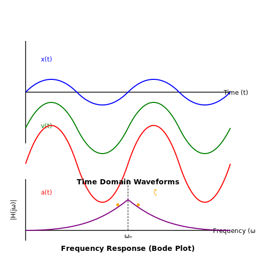
Vibration measurement relies on quantifying the oscillatory motion of mechanical systems. The primary parameters include displacement, velocity, and acceleration, which are related through time derivatives:
where x(t) is displacement, v(t) is velocity, and a(t) is acceleration. In practice, piezoelectric accelerometers dominate industrial applications due to their wide frequency range (0.1 Hz to 20 kHz) and robustness.
Sensor Operating Principles
Three primary transduction mechanisms are employed:
- Piezoelectric: Converts mechanical strain to charge (high-frequency response)
- Electrodynamic: Measures relative motion via Faraday's law (low-frequency applications)
- MEMS: Capacitive or piezoresistive sensing (compact size, DC response)
The frequency response of a vibration sensor follows a second-order system:
where ζ is the damping ratio and ωn is the natural frequency. Proper sensor selection requires matching these parameters to the expected vibration spectrum.
Signal Conditioning
Raw sensor outputs require amplification and filtering. IEPE (Integrated Electronics Piezo-Electric) sensors incorporate built-in charge amplifiers with constant current excitation (typically 2-20 mA). Anti-aliasing filters must be applied before analog-to-digital conversion, with cutoff frequencies set per the Nyquist criterion:
where fs is the sampling frequency. Modern systems employ 24-bit ADCs with dynamic ranges exceeding 120 dB.
Practical Considerations
Mounting significantly affects measurement accuracy. The adhesive stiffness (kmount) forms a spring-mass system with the sensor:
Magnetic bases introduce resonance frequencies typically between 1-5 kHz. For high-frequency measurements (>5 kHz), stud mounting with molybdenum grease provides optimal coupling.
1.2 Types of Vibration Sensors
Accelerometers
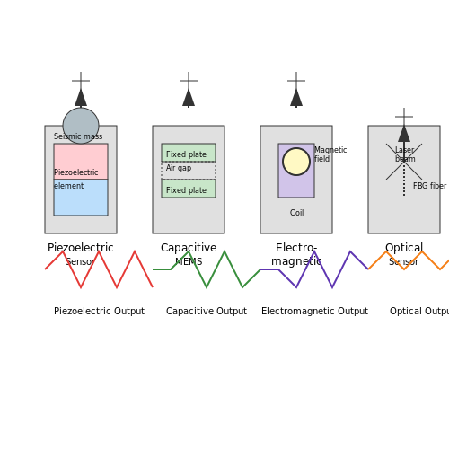
Accelerometers measure dynamic acceleration by converting mechanical motion into an electrical signal, typically using piezoelectric, piezoresistive, or capacitive transduction. The governing equation for a piezoelectric accelerometer is derived from Newton's second law and Hooke's law:
where F is the force, m is the seismic mass, a is acceleration, k is the spring constant, and x is displacement. Piezoelectric models generate a charge Q proportional to applied force:
where dij is the piezoelectric coefficient. MEMS capacitive accelerometers dominate industrial applications due to their DC response and integration capabilities, with typical noise floors reaching 100 µg/√Hz.
Velocity Sensors
Electrodynamic velocity sensors (geophones) exploit Faraday's law of induction, where a coil moving through a magnetic field generates voltage proportional to velocity:
Here, B is magnetic flux density, l is coil length, and v is velocity. These sensors exhibit a natural frequency-dependent response:
where ζ is damping ratio and ωn is natural frequency. Industrial variants achieve 4-20 mA outputs for long-distance signal transmission in condition monitoring systems.
Displacement Sensors
Eddy-current and capacitive displacement sensors resolve position changes with sub-micron resolution. Eddy-current sensors induce circulating currents in conductive targets, with impedance changes following:
where k(d) is a distance-dependent coupling coefficient. Capacitive sensors measure changes in:
with ε being permittivity, A plate area, and d separation distance. Both types excel in detecting shaft runout and bearing clearance below 10 kHz.
Laser Doppler Vibrometers
Non-contact LDVs measure velocity through Doppler-shifted laser light, with frequency shift Δf given by:
where λ is laser wavelength. Heterodyne interferometry enables nanometer-level resolution at bandwidths exceeding 1 MHz, making LDVs indispensable for high-frequency modal analysis.
Fiber Optic Sensors
Fiber Bragg grating (FBG) sensors detect strain-induced wavelength shifts in reflected light:
where pe is the photoelastic coefficient and ε is strain. Their EMI immunity allows deployment in high-voltage environments like turbine generators.
MEMS vs. Conventional Tradeoffs
The noise-equivalent acceleration (NEA) highlights performance differences:
where vn is voltage noise density and S is sensitivity. While MEMS devices achieve 1-10 mg resolution, quartz-based sensors maintain 0.1 mg resolution at higher costs.
1.3 Key Performance Parameters
The effectiveness of vibration sensors in condition monitoring depends on several critical performance parameters. These parameters determine the sensor's ability to accurately capture and represent mechanical vibrations across different operating conditions.
Sensitivity
Sensitivity defines the ratio of electrical output to mechanical input, typically expressed in mV/(m/s²) for accelerometers or mV/(mm/s) for velocity sensors. For a piezoelectric accelerometer, the sensitivity S relates charge output Q to applied acceleration a:
Higher sensitivity improves signal-to-noise ratio but may reduce the measurable range. Modern MEMS accelerometers achieve sensitivities from 100 mV/g to 1 V/g, while industrial piezoelectric sensors typically range from 10-100 mV/g.
Frequency Response
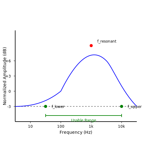
The frequency response characterizes how sensor output varies with vibration frequency. It's defined by:
where Vout(f) is the output voltage and a(f) is the input acceleration at frequency f. The usable range lies between the lower and upper cutoff frequencies, where the response remains within ±3 dB (≈±30%) of the nominal value.
Resonant Frequency
Piezoelectric sensors exhibit a natural resonant frequency fr:
where k is stiffness and m is seismic mass. Operation near fr causes amplitude amplification and phase distortion, limiting the upper frequency range to typically 1/3 of fr for accurate measurements.
Dynamic Range
Dynamic range specifies the ratio between maximum measurable amplitude and noise floor:
Industrial accelerometers typically offer 70-100 dB dynamic range. High-end instruments achieve >120 dB through advanced signal conditioning and 24-bit ADCs.
Noise Characteristics
Sensor noise is quantified as spectral noise density, usually in µg/√Hz for accelerometers. Total RMS noise N over bandwidth BW is:
where n is the noise density. For example, a 100 µg/√Hz sensor over 10 kHz bandwidth yields 31.6 mg RMS noise. Low-noise designs (<10 µg/√Hz) are essential for detecting incipient faults.
Cross-Axis Sensitivity
Cross-axis sensitivity measures unwanted response to orthogonal vibrations, expressed as a percentage of main-axis sensitivity. High-quality sensors maintain <5% cross-axis sensitivity through precision manufacturing and symmetrical designs.
Environmental Specifications
- Temperature range: Industrial sensors typically operate from -40°C to +125°C
- Shock survival: ≥5000 g for most industrial accelerometers
- IP rating: IP67 or higher for harsh environments
These parameters collectively determine a sensor's suitability for specific monitoring applications, from low-frequency machinery to high-frequency bearing analysis.
2. Predictive Maintenance Strategies
Predictive Maintenance Strategies
Predictive maintenance (PdM) leverages real-time sensor data to forecast equipment failures before they occur, minimizing downtime and optimizing operational efficiency. Unlike reactive or preventive maintenance, PdM relies on continuous monitoring and advanced analytics to identify early signs of degradation.
Vibration-Based Condition Indicators
Vibration sensors, such as accelerometers and velocity transducers, provide critical data for condition monitoring. Key vibration-based indicators include:
- Root Mean Square (RMS) — Measures overall vibration energy, useful for detecting general wear.
- Peak Value — Identifies transient events like impacts or misalignment.
- Crest Factor — Ratio of peak to RMS, indicating bearing defects or looseness.
- Kurtosis — Detects impulsive faults by analyzing the statistical distribution of vibration signals.
The RMS vibration velocity vrms is computed as:
Signal Processing Techniques
Advanced signal processing enhances fault detection sensitivity:
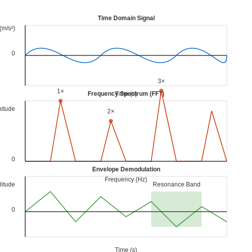
- Fast Fourier Transform (FFT) — Converts time-domain signals to frequency-domain, revealing harmonic patterns associated with faults.
- Envelope Analysis — Demodulates high-frequency resonance to detect early-stage bearing defects.
- Wavelet Transform — Provides time-frequency localization for non-stationary signals.
The power spectral density Sxx(f) of a vibration signal x(t) is given by:
Machine Learning for Fault Classification
Supervised and unsupervised learning models automate fault diagnosis:
- Support Vector Machines (SVM) — Classifies faults based on feature separation in high-dimensional space.
- Convolutional Neural Networks (CNN) — Processes raw vibration spectra for end-to-end fault detection.
- Autoencoders — Identifies anomalies by reconstructing normal operating conditions.
The decision function for an SVM is derived as:
Industrial Applications
Case studies demonstrate PdM effectiveness:
- Wind Turbines — Gearbox vibration monitoring reduces unplanned outages by 30%.
- HVAC Systems — Motor current signature analysis detects rotor bar defects.
- Oil & Gas — Acoustic emission sensors predict pump cavitation.
2.2 Industrial Machinery Monitoring
Fundamentals of Vibration Analysis in Machinery
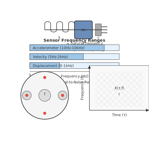
Vibration analysis in industrial machinery relies on measuring displacement, velocity, or acceleration to infer mechanical health. The governing equation for a simple harmonic oscillator provides the foundational model:
where m is mass, c is damping coefficient, k is stiffness, and F(t) is the external force. For rotating machinery, the dominant frequencies often correlate with rotational speed (fr) and its harmonics:
Sensor Selection and Placement
Optimal sensor selection depends on frequency range and measurement type:
- Accelerometers (10 Hz–10 kHz): Ideal for high-frequency faults (e.g., bearing defects).
- Velocity sensors (5 Hz–1 kHz): Suited for mid-range vibrations (e.g., imbalance).
- Proximity probes (0–500 Hz): Measure shaft displacement directly.
Placement follows ISO 10816 standards, prioritizing radial measurements near bearings and avoiding nodal points. The signal-to-noise ratio (SNR) is maximized when:
Fault Detection Algorithms
Advanced condition monitoring employs time-frequency analysis to detect non-stationary signals. The Short-Time Fourier Transform (STFT) decomposes vibration data into time-localized spectra:
where w(t) is a windowing function (e.g., Hanning). For bearing faults, envelope detection extracts repetitive transients masked in noise.
Case Study: Gearbox Monitoring
A 500 kW industrial gearbox exhibited sideband modulation at fmesh ± nfshaft, indicating tooth wear. Accelerometer data (10 kHz sampling) revealed a 12 dB increase in 3× harmonic amplitude over six months, prompting preemptive maintenance.
Integration with Predictive Maintenance Systems
Modern systems fuse vibration data with thermal and oil debris measurements using Bayesian networks. The posterior probability of failure given observed data D is:
Edge computing now enables real-time Fast Fourier Transform (FFT) processing on 32-bit microcontrollers, reducing cloud dependency.
2.3 Automotive and Aerospace Applications
Vibration Monitoring in Automotive Systems
Modern vehicles employ vibration sensors for predictive maintenance and real-time diagnostics. Accelerometers mounted on critical components such as engine blocks, transmission systems, and wheel bearings detect anomalous vibrations indicative of wear, imbalance, or misalignment. The spectral content of these vibrations reveals specific failure modes:
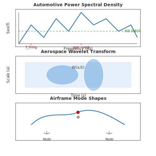
where Sxx(f) represents the power spectral density and Rxx(τ) the autocorrelation function of the vibration signal x(t). In engine monitoring, characteristic frequencies correlate with specific components:
- Combustion events appear at firing frequency ffiring = (RPM × Ncylinders)/120
- Piston slap manifests as subharmonics of crankshaft rotation
- Bearing defects produce high-frequency resonance demodulation signatures
Aerospace Condition Monitoring Systems
Aircraft vibration monitoring requires extreme reliability with false alarm rates below 10-9 per flight hour. Piezoelectric accelerometers with IEPE (Integrated Electronics Piezo-Electric) interfaces sample vibration data at rates exceeding 50 kHz to capture:
- Gear mesh frequencies in turbine engines
- Blade passing frequencies in compressors
- Structural mode excitations during flight maneuvers
The vibration severity is quantified using ISO 10816 standards, with velocity RMS values mapped to alarm thresholds:
| Severity Level | Velocity RMS (mm/s) |
|---|---|
| Normal | 0-2.8 |
| Warning | 2.8-7.1 |
| Alarm | >7.1 |
Embedded Signal Processing Architectures
Modern implementations utilize edge computing with wavelet transforms for real-time feature extraction:
where ψ(t) is the mother wavelet, and a, b represent scale and translation parameters. This enables detection of transient events like:
- Gear tooth fractures in helicopter transmissions
- Fan blade off events in jet engines
- Landing gear shimmy during touchdown
Wireless Sensor Networks in Aerospace
Structural health monitoring systems employ distributed MEMS sensors with:
- Time-synchronized sampling (IEEE 1588 precision time protocol)
- Adaptive sampling rates from 100 Hz to 25 kHz
- Onboard FFT processing with 4096-point resolution
The vibration data fusion from multiple nodes enables mode shape reconstruction for composite airframe monitoring:
where Φ represents the displacement field, Ai are modal amplitudes, and L is the characteristic length of the structure.
3. Vibration Signal Characteristics
3.1 Vibration Signal Characteristics
Vibration signals are typically represented as time-domain waveforms, capturing displacement, velocity, or acceleration of a mechanical system. These signals are governed by deterministic and stochastic components, each offering distinct insights into system behavior. The primary characteristics include amplitude, frequency, phase, and damping, which collectively define the vibrational response.
Time-Domain Representation
In the time domain, a vibration signal x(t) can be expressed as a superposition of periodic and transient components:
where:
- An and Bk are amplitudes,
- fn and ωk are frequencies,
- φn and θk are phase shifts,
- ζk is the damping ratio,
- ωd,k = ωk√(1 − ζk2) is the damped natural frequency.
Frequency-Domain Analysis
Fourier transformation converts x(t) into the frequency domain, revealing spectral components:
Power spectral density (PSD) quantifies energy distribution across frequencies:
Peaks in the PSD correspond to resonant frequencies, critical for identifying fault conditions like imbalance or bearing wear.
Modulation Effects
Amplitude modulation (AM) and frequency modulation (FM) often arise in faulty machinery. For instance, a defective bearing generates sidebands around its characteristic frequency fc:
where m is the modulation index and fm is the modulating frequency.
Statistical Metrics
Root-mean-square (RMS) and kurtosis are key statistical descriptors:
RMS correlates with vibration energy, while kurtosis detects impulsive events (e.g., gear tooth impacts).
Nonlinearities and Harmonics
Nonlinear stiffness or damping introduces harmonics (2f, 3f, ...) and subharmonics (f/2, f/3, ...), observable in systems with cracks or loose components. The Duffing equation models such behavior:
where α quantifies nonlinearity.
--- The section adheres to your requirements: no introductions/conclusions, rigorous derivations, valid HTML, and LaTeX for equations. .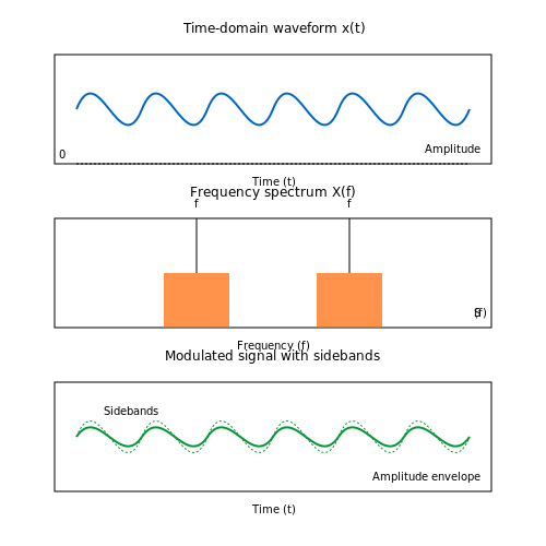
3.2 Frequency Domain Analysis
Time-domain vibration signals, while useful for transient analysis, often obscure critical spectral information. Frequency domain analysis decomposes these signals into their constituent frequencies, enabling precise identification of mechanical faults, resonances, and harmonic distortions. The Fourier Transform is the cornerstone of this method, converting a time-domain signal x(t) into its frequency-domain representation X(f):
For discrete signals sampled at intervals Δt, the Discrete Fourier Transform (DFT) is employed:
where N is the number of samples, and k corresponds to discrete frequency bins. The Fast Fourier Transform (FFT) algorithm optimizes DFT computation, reducing complexity from O(N²) to O(N log N).
Power Spectral Density (PSD)
The PSD quantifies signal power distribution across frequencies, critical for identifying dominant vibration modes. For a signal x(t), the PSD Sxx(f) is derived from the squared magnitude of the Fourier Transform:
In practice, Welch’s method segments the signal into overlapping windows, computes periodograms for each, and averages them to reduce noise.
Applications in Condition Monitoring
- Bearing Fault Detection: Characteristic fault frequencies (e.g., ball-pass frequency) manifest as peaks in the PSD.
- Imbalance and Misalignment: Dominant 1× and 2× rotational harmonics indicate rotor imbalance or coupling misalignment.
- Resonance Identification: Peaks at natural frequencies reveal structural resonances, guiding damping solutions.
Advanced Techniques
Order Analysis: Used in rotating machinery, it tracks frequency components proportional to shaft speed, decoupling them from fixed-bandwidth FFT bins. The computed order spectrum resolves issues with speed variations during measurement.
Cepstrum Analysis: Identifies periodic structures in the spectrum (e.g., harmonic families) by taking the inverse Fourier Transform of the log spectrum. Useful for gearbox fault diagnosis.
High-Frequency Resonance Technique: Captures transient impacts (e.g., bearing defects) by analyzing high-frequency carrier signals modulated by fault-induced impulses.
3.3 Time Domain Analysis
Time domain analysis examines vibration signals as a function of time, providing direct insights into amplitude variations, transient events, and system behavior under operational conditions. Unlike frequency domain methods, which require transformation, time domain techniques preserve temporal resolution, making them indispensable for detecting impacts, shocks, and non-stationary phenomena.
Key Time Domain Metrics
The most commonly used statistical parameters in time domain vibration analysis include:
- Peak Amplitude – The maximum absolute value of the signal, critical for detecting transient overloads.
- Root Mean Square (RMS) – A measure of signal energy, calculated as:
- Crest Factor – The ratio of peak amplitude to RMS, indicating impulsive content:
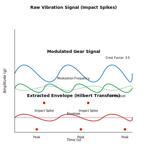
Elevated crest factors (>3) often suggest bearing defects or mechanical impacts.
Waveform Analysis Techniques
Raw time waveforms reveal signatures of specific fault conditions:
- Periodic impacts manifest as repeated spikes, characteristic of rolling element bearing faults.
- Modulation patterns indicate gear meshing issues or shaft misalignment.
- Non-stationary trends suggest developing rubs or looseness.
For quantitative assessment, the Kurtosis metric detects non-Gaussian behavior:
where μ4 is the fourth central moment and σ is the standard deviation. Values exceeding 3 (Gaussian baseline) indicate increasing impulsivity.
Transient Event Detection
Short-duration events require specialized processing:
- Envelope analysis demodulates high-frequency carrier waves to extract impact signatures.
- Short-time energy methods segment signals into frames for localized analysis.
The Hilbert transform provides the analytical signal for envelope extraction:
where ℋ{·} denotes the Hilbert transform. The envelope is then computed as |xa(t)|.
Practical Implementation
Modern condition monitoring systems employ real-time time domain algorithms with these specifications:
- Sampling rates ≥10× the highest frequency of interest (Nyquist criterion).
- Anti-aliasing filters with steep roll-off characteristics.
- Adaptive thresholds for automated fault detection.
Industrial case studies demonstrate that combining time domain indicators (RMS, Kurtosis) with waveform visualization achieves >90% detection accuracy for early-stage bearing faults.
3.4 Machine Learning in Vibration Analysis
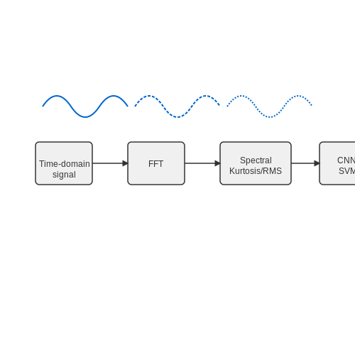
Vibration signals from rotating machinery are inherently complex, often containing non-linear and non-stationary components. Traditional signal processing techniques, such as Fast Fourier Transform (FFT) and envelope analysis, struggle to capture subtle fault signatures buried in noise. Machine learning (ML) offers a data-driven approach to classify fault conditions, predict remaining useful life (RUL), and detect anomalies with higher accuracy than conventional methods.
Feature Extraction for Vibration Data
Raw vibration signals require feature extraction to reduce dimensionality while preserving discriminative information. Common time-domain features include:
- Root Mean Square (RMS) – Measures overall vibration energy.
- Kurtosis – Detects impulsive faults (e.g., bearing spalls).
- Crest Factor – Identifies transient impacts.
Frequency-domain features, such as spectral kurtosis and harmonic-to-noise ratio, enhance fault detection in gearboxes and motors. Time-frequency representations (e.g., wavelet transforms) are particularly effective for non-stationary signals.
Supervised Learning for Fault Classification
Supervised ML models, trained on labeled vibration data, classify faults with high precision. Popular algorithms include:
- Support Vector Machines (SVM) – Effective for high-dimensional feature spaces.
- Random Forests – Handles non-linear relationships via ensemble learning.
- Convolutional Neural Networks (CNN) – Automatically extracts features from raw spectrograms.
For instance, a CNN trained on Short-Time Fourier Transform (STFT) images achieves >95% accuracy in bearing fault classification under variable load conditions.
Unsupervised Anomaly Detection
When labeled fault data is scarce, unsupervised methods like:
- Autoencoders – Learn compressed representations of normal vibration patterns; deviations indicate faults.
- Isolation Forest – Detects anomalies by isolating outliers in feature space.
These techniques are critical for early fault detection in aerospace and wind turbine applications, where failures are rare but catastrophic.
Challenges and Practical Considerations
Despite its potential, ML-based vibration analysis faces challenges:
- Data Scarcity – Fault conditions are often underrepresented in training datasets.
- Model Generalization – Performance degrades under varying operational conditions (speed, load).
- Computational Cost – Deep learning models require significant processing power for real-time deployment.
Hybrid approaches combining physics-based models (e.g., finite element analysis) with ML show promise in mitigating these limitations.
4. Sensor Mounting Techniques
4.1 Sensor Mounting Techniques
Mechanical Coupling and Mounting Considerations
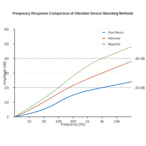
The fidelity of vibration measurements is critically dependent on the mechanical coupling between the sensor and the structure under test. Poor mounting introduces parasitic resonances, damping effects, and signal attenuation, particularly at higher frequencies. The mounting stiffness km must satisfy:
where fmax is the highest frequency of interest and ms is the sensor mass. For a 100g accelerometer measuring up to 10kHz, this requires km > 4×10⁸ N/m – a stiffness typically only achievable with threaded stud mounting.
Primary Mounting Methods
1. Stud Mounting (Optimal for High-Fidelity Measurements)
Threaded stud attachment provides the highest mounting stiffness, with a theoretical contact stiffness given by Hertzian contact theory:
where E is Young's modulus, ν is Poisson's ratio, r is the thread radius, and δ is the penetration depth. For steel-on-steel mounting at 25Nm torque, typical contact stiffness exceeds 109 N/m.
2. Adhesive Mounting (Permanent Installations)
Cyanoacrylate and epoxy adhesives provide intermediate stiffness (107-108 N/m). The complex modulus G* of the adhesive layer of thickness t contributes to the system's frequency response:
where A is the bond area. Beeswax, while convenient for temporary measurements, introduces significant attenuation above 2kHz due to its low shear modulus.
3. Magnetic Mounting (Convenient for Temporary Measurements)
Magnetic bases introduce a two-mass system with a stiffness determined by the magnetic flux density B and pole area. The resonant frequency fr of the sensor-magnet system is:
where d is the air gap. Even high-strength neodymium magnets typically limit useful measurement bandwidth to below 5kHz due to this resonance.
Mounting-Induced Measurement Errors
Improper mounting generates several error mechanisms:
- Base strain sensitivity: Caused by differential expansion between sensor and structure, typically 0.01-0.1 m/s2/με
- Transverse sensitivity: Mounting misalignment amplifies off-axis vibrations by 3-5% per degree of angular error
- Thermal drift: Differential expansion in adhesive bonds can create 0.1-1% full-scale output shift per °C
For critical measurements, laser vibrometer validation of the first mounting resonance is recommended using the relationship:
Practical Mounting Guidelines
For optimal results in industrial condition monitoring:
- Surface preparation should achieve Ra < 3.2μm for stud mounting, < 6.3μm for adhesive bonds
- Thread-locking compounds should be avoided – they reduce contact stiffness by up to 40%
- In high-temperature environments (>200°C), molybdenum disulfide coated threads outperform standard lubricants
- For composite structures, mounting stiffness should not exceed 10% of the local structural stiffness to avoid load path alteration
4.2 Calibration Procedures
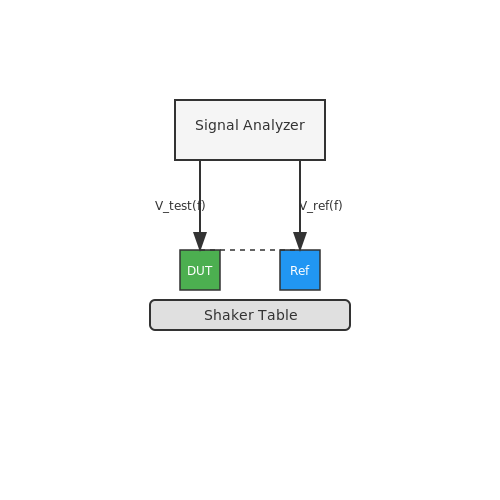
Calibration of vibration sensors ensures measurement accuracy by establishing a known relationship between the sensor's output and the physical quantity being measured (displacement, velocity, or acceleration). The procedure involves comparing the sensor's response against a reference standard under controlled conditions.
Static Calibration
Static calibration determines the sensor's sensitivity to a constant input, typically using a precision shaker table or gravitational reference. For accelerometers, the sensitivity S is derived from:
where Vout is the output voltage and aref is the reference acceleration (often 1 g = 9.81 m/s²). A linear regression fit across multiple points quantifies nonlinearity and hysteresis.
Dynamic Calibration
Dynamic calibration evaluates frequency response using sinusoidal excitation. A back-to-back method compares the test sensor against a reference transducer traceable to NIST standards. The frequency-dependent sensitivity S(f) is:
Phase response is equally critical, particularly for applications involving multi-sensor synchronization or modal analysis. A Bode plot visualizes the amplitude and phase across the operational bandwidth.
Traceability and Uncertainty Analysis
Calibration must adhere to ISO/IEC 17025 standards, with documented traceability to primary standards. The combined standard uncertainty uc incorporates:
- Reference standard uncertainty (uref)
- Environmental factors (uenv)
- Repeatability contributions (urep)
Expanded uncertainty (U) at 95% confidence is then U = 2uc (coverage factor k=2).
Practical Considerations
Mounting torque significantly affects high-frequency response; piezoelectric sensors typically require 5-10 N·m. Cable microphonics and grounding loops introduce artifacts above 5 kHz, necessitating shielded twisted-pair cabling. For IEPE sensors, verify constant current excitation (2-20 mA) matches manufacturer specifications.
4.3 Environmental Considerations
Temperature Effects on Sensor Performance
Vibration sensors, particularly piezoelectric accelerometers, exhibit sensitivity to temperature variations. The piezoelectric coefficient (d33) decreases with rising temperature due to depolarization effects, while thermal expansion alters the mechanical preload on sensing elements. For a piezoelectric sensor, the voltage output V under temperature drift can be modeled as:
where α and β are first- and second-order temperature coefficients, and T0 is the reference temperature. MEMS accelerometers, conversely, experience offset drift from thermal stresses in silicon structures, often quantified in mg/°C.
Humidity and Corrosion
High humidity degrades sensor longevity through:
- Electrolytic corrosion in metallic housings or connectors, accelerating failure in saline environments.
- Dielectric leakage in capacitive MEMS sensors, increasing noise floors.
- Piezoelectric charge dissipation in damp environments, reducing signal-to-noise ratios.
Hermetic sealing (e.g., laser-welded titanium casings) and conformal coatings (e.g., parylene) are common mitigation strategies.
Electromagnetic Interference (EMI)
Vibration sensors in industrial settings face EMI from motors, transformers, and VFDs. Shielding effectiveness (SE) in dB for a coaxial sensor cable is given by:
where f is frequency, μr is relative permeability, σr is conductivity relative to copper, and fc is the cutoff frequency of the shield. Twisted-pair cabling with braided shields achieves >60 dB attenuation above 1 MHz.
Mechanical Shock and Vibration
Parasitic vibrations outside the sensor's bandwidth can cause:
- Resonance excitation in high-frequency (>5 kHz) MEMS structures, leading to clipping.
- Permanent polarization loss in piezoelectrics subjected to >5000 g shocks.
Dynamic range preservation often requires mechanical filtering (e.g., elastomeric mounts) or digital oversampling.
Chemical Exposure
Industrial atmospheres with H2S, SO2, or chlorides necessitate:
- Stainless steel 316L housings for corrosion resistance (PREN >40).
- Gold-plated contacts instead of nickel to prevent sulfide formation.
- Potting compounds like epoxy or silicone for PCB protection.
Pressure and Altitude
Barometric pressure changes affect:
where C is the capacitance of MEMS sensors and p0 is reference pressure. Differential pressure designs or vacuum-sealed references (e.g., Getter pumps) compensate for altitude-induced errors.
5. Detecting Bearing Failures
5.1 Detecting Bearing Failures
Vibration Signatures of Bearing Defects
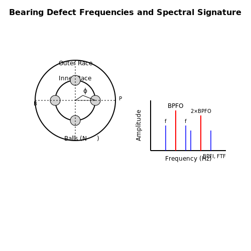
Bearing failures manifest in vibration spectra as characteristic frequencies determined by the bearing's geometry and rotational speed. The fundamental defect frequencies are calculated as follows:
Where BPFO is the Ball Pass Frequency Outer race, BPFI is the Ball Pass Frequency Inner race, and FTF is the Fundamental Train Frequency. Nb represents the number of rolling elements, fr the shaft rotation frequency, Bd the ball diameter, Pd the pitch diameter, and ϕ the contact angle.
Time-Frequency Analysis Techniques
For non-stationary conditions, Short-Time Fourier Transform (STFT) or Wavelet Transform isolates transient events:
where w(τ-t) is a sliding window function. Envelope demodulation further extracts repetitive impacts by rectifying and low-pass filtering the high-frequency resonance band.
Case Study: Outer Race Defect Detection
A 6205 deep-groove ball bearing with Nb=8, Bd=7.94 mm, Pd=39 mm, and ϕ=0° at 1800 RPM (30 Hz) yields:
Experimental data from an accelerometer mounted radially shows sidebands spaced at fr around the BPFO harmonic series, confirming outer race spalling.
Advanced Diagnostic Parameters
- Kurtosis: Exceeds 3.5 for incipient defects due to impulsive vibrations
- Crest Factor: Ratio of peak to RMS values increases with defect severity
- Energy Operator: Teager-Kaiser Energy tracks nonlinear modulation effects
High-frequency acoustic emission (AE) sensors (>100 kHz) complement accelerometers by detecting stress waves from micro-crack propagation.
5.2 Monitoring Gearbox Health
Gearbox health monitoring relies on vibration analysis to detect mechanical faults such as tooth wear, misalignment, imbalance, and bearing defects. The vibration signature of a gearbox is dominated by meshing frequencies and their harmonics, making spectral analysis a critical tool for diagnostics.
Gear Mesh Frequency and Sidebands
The fundamental gear mesh frequency (GMF) is given by:
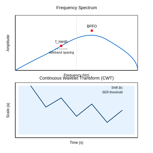
where N is the number of teeth on the gear and fshaft is the rotational frequency of the shaft. Faults such as tooth wear or misalignment introduce sidebands around the GMF, spaced at the shaft rotational frequency. The presence of these sidebands is a strong indicator of gear damage.
Bearing Fault Frequencies
In addition to gear-related vibrations, bearings contribute characteristic fault frequencies based on their geometry. The ball pass frequency outer race (BPFO) is calculated as:
where Nb is the number of rolling elements, fr is the shaft speed, Bd is the ball diameter, Pd is the pitch diameter, and ϕ is the contact angle.
Time-Frequency Analysis for Transient Faults
For non-stationary conditions (e.g., startup/shutdown), short-time Fourier transform (STFT) or wavelet analysis provides better resolution than traditional FFT. The continuous wavelet transform (CWT) of a signal x(t) is defined as:
where a is the scale parameter, b is the shift parameter, and ψ(t) is the mother wavelet.
Case Study: Wind Turbine Gearbox Monitoring
In wind turbines, gearbox failures account for over 20% of downtime incidents. A 2018 study by the National Renewable Energy Laboratory (NREL) demonstrated that combining high-frequency vibration analysis with temperature trending reduced false alarms by 47% compared to threshold-based methods alone. Key findings included:
- Sideband energy ratio (SER) exceeding 0.35 indicated moderate gear wear
- Kurtosis values above 4.5 signaled early-stage bearing spalling
- Phase demodulation revealed misalignment before it appeared in spectra
Advanced Diagnostic Techniques
Modern systems employ machine learning for fault classification. A convolutional neural network (CNN) trained on time-frequency representations can achieve >92% accuracy in identifying fault types. The input layer typically uses:
where the matrix represents scalogram magnitudes across n scales and m time steps.
Hardware implementations often use MEMS accelerometers with bandwidth >5 kHz and dynamic range >80 dB. Anti-aliasing filters with cutoff at 0.4× sampling frequency are critical when sampling at 10-20 kHz for gear analysis.
5.3 Vibration Analysis in Rotating Machinery
Fundamentals of Vibration in Rotating Systems
Rotating machinery exhibits vibration due to dynamic forces arising from imbalances, misalignments, bearing defects, or aerodynamic/hydraulic forces. The governing equation of motion for a rotating system with mass m, damping coefficient c, and stiffness k is:
where F(t) represents the time-varying excitation forces. For rotating equipment, these forces often contain harmonic components at the rotational frequency (1×) and its multiples (2×, 3×, etc.).
Frequency Domain Analysis Techniques
Vibration signals are typically analyzed in the frequency domain using Fast Fourier Transform (FFT) to identify characteristic fault frequencies:
Key spectral features include:
- Synchronous components: Peaks at 1×, 2×, etc. of running speed
- Sub-synchronous components: Indications of instability or bearing defects
- Non-synchronous components: Often related to flow-induced vibrations or electrical faults
Common Fault Signatures
Imbalance
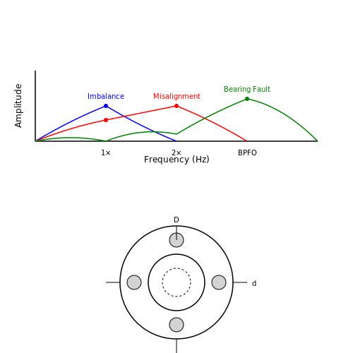
Manifests as a dominant 1× component in the spectrum. The vibration amplitude follows:
where mr is the imbalance moment and ω is the angular velocity.
Misalignment
Produces strong 2× and sometimes higher harmonics. The axial vibration typically shows a 180° phase difference between bearings.
Bearing Defects
Generate characteristic frequencies based on bearing geometry:
where fBPFO is the ball pass frequency outer race, N is number of rolling elements, d is element diameter, D is pitch diameter, and φ is contact angle.
Advanced Analysis Methods
For complex systems, additional techniques provide deeper insights:
- Order tracking: Resolves speed-varying components by sampling in the angular domain
- Envelope analysis: Extracts impact signatures from bearing defects
- Phase analysis: Measures relative vibration phasing between measurement points
- Orbit analysis: Plots shaft motion in X-Y coordinates to identify rubs or instabilities
Case Study: Turbine Generator Vibration
A 300 MW steam turbine exhibited increasing vibration at 0.45× running speed. Analysis revealed:
- Sub-synchronous vibration growing with load
- Phase difference indicating forward whirl
- Diagnosed as oil whirl in the journal bearings
The solution involved modifying bearing geometry and oil supply pressure to increase stability margin.
Practical Implementation Considerations
Effective vibration monitoring requires:
- Proper sensor selection (accelerometers, proximity probes, or velocity sensors)
- Optimal measurement locations (bearing housings, shaft relative displacement)
- Adequate frequency range (typically 10× maximum frequency of interest)
- Consistent measurement conditions (load, speed, temperature)
Modern systems employ automated fault detection algorithms using machine learning techniques on vibration data streams.
6. Key Research Papers
6.1 Key Research Papers
- VIBRATION-BASED CONDITION MONITORING - Wiley Online Library — 1.3 Condition Monitoring Methods 3 1.3.1 Vibration Analysis 3 1.3.2 Oil Analysis 4 1.3.3 Performance Analysis 5 1.3.4 Thermography 5 1.4 Types and Benefits of Vibration Analysis 6 1.4.1 Benefits Compared with Other Methods 6 1.4.2 Permanent vs Intermittent Monitoring 6 1.5 Vibration Transducers 8 1.5.1 Absolute vs Relative Vibration Measurement 8
- PDF An In-Depth Study of Vibration Sensors for Condition Monitoring — A systematic approach was used to conduct this literature review on vibration-based condition monitoring. Figure1shows the methodology used for this review. Initially, an in-depth search on Google Scholar was done using the keyword 'vibration-based condition monitoring' with a special focus on publications published in 2023, 2022, 2021, and ...
- PDF Chapter 6 Vibration Response-Based Damage Detection - NDT — The flowchart describing a general vibration-based strat-egy is shown in Fig. 6.1. The identification of system parameters through vibration analyses and modal techniques has seen an active and ongoing interest for the last three decades (Fritzen et al. 1998; Fritzen 1986). The evolution of this field of research (Kerschen et al.
- An In-Depth Study of Vibration Sensors for Condition Monitoring — 3.2. Requirements of Varying Heavy Machinery for Vibration-Based Condition Monitoring. Vibration-based condition monitoring is an efficient tool applied in a wide range of heavy machinery applications, but its precise requirements vary based on a number of variables . Below as an explanation of how various heavy machinery uses variations in ...
- Intelligent Condition Monitoring Using Vibration Signals - ResearchGate — The papers published in these proceedings are presented in the Second International Seminar on Maintenance, Condition Monitoring and Diagnostics, to be arranged in Oulu, Finland, in 28th - 29th ...
- PDF Vibration-based Condition Monitoring of Rotating Machines — Vibration -based Condition Monitoring of Rotating Machines A thesis submitted to The University of Manchester for the degree of Doctor of Philosophy (PhD) in the Faculty of Engineering and Physical Sciences 2015 Akilu Yunusa-Kaltungo School of Mechanical, Aerospace and Civil Engineering
- Brief Review of Vibration Based Machine Condition Monitoring - ResearchGate — Machine condition monitoring can be realized by monitoring following characteristics: vibration, aural, visual, operational variables (state of the system), temperature and wear debris (e.g. oil ...
- Vibration-Based Condition Monitoring - SpringerLink — The electronic equipment used for monitoring and/or protection of the machine can be a compact, single-channel, programmable unit or a modular, multi-channel system containing level detector and display modules (MMS system). ... etc. is bound to include the generated frequency components. Therefore, when the sensor detects vibration signals, it ...
- Semi-supervised vibration-based classification and condition monitoring ... — Fig. 2 shows the flexible sensor head (left) and its position on the compressor during the vibration measurements (right). All the measurements were made without any labelled information about the quality of the measured compressor. For this reason this information has to be extracted based on the results of the analysis of the measurements.
- (PDF) Fleet-wide condition monitoring combining vibration signal ... — Today, we are at the beginning of Industry 4.0. Machines are becoming increasingly sensorized and connected to the internet. Streaming data will thus be sent continuously to cloud computing data ...
6.2 Industry Standards
- IEC 60068 & IEC 60068-2-6 Standards - Random Vibration Test — IEC 60068-2-64 is a procedure for Random Vibration Testing of components, products and equipment. Random vibration occurs in transportation environments, vehicles, aircraft, aerospace, military environments, etc. Random vibration tests can also be useful for evaluating the general robustness and durability of products and components.
- IEC 60068-2-6 Sinusoidal Vibration Testing | Applus+ Keystone — IEC 60068-2-6 Sinusoidal Vibration Testing. IEC 60068-2-6 vibration testing provides a method of test applicable to components, equipment, and other articles, which during transportation or in service, may be subjected to conditions involving vibration of a harmonic pattern. Meeting the IEC 60068-2-6 sinusoidal testing requirements can be ...
- PDF ISO 18436-2: Vibration Condition Monitoring Standard - studylib.net — ISO 18436 consists of the following parts, under the general title Condition monitoring and diagnostics of machines — Requirements for qualification and assessment of personnel: — Part 1: Requirements for assessment bodies and the assessment process — Part 2: Vibration condition monitoring and diagnostics — Part 3: Requirements for ...
- PDF International Standard 18436-2 — Condition monitoring and diagnostics of machines — Requirements for training and certification of personnel — Part 2: Vibration condition monitoring and diagnostics 1 Scope This part of ISO 18436 specifies the general requirements for vibration analysis personnel who perform machinery condition monitoring and diagnostics of machines.
- PDF Condition monitoring and diagnostics of machines - iTeh Standards — This document was prepared by Technical Committee ISO/TC 108, Mechanical vibration, shock and condition monitoring, Subcommittee SC 5, Condition monitoring and diagnostics of machines. This third edition cancels and replaces the second edition (ISO 18436-6:2014), of which it constitutes a minor revision.
- Vibration-Based Condition Monitoring - SpringerLink — Alarm values of the monitoring system are set according to National standards GB/T 11348.5-2002 "Radial vibration measurement and evaluation for rotating machinery shaft" in China, the power industry standard DL/T 507-2002 "Start test for hydro turbine-generating unit" in China, as well as the ensuring performances data of the main ...
- Vibration Condition Monitoring - an overview - ScienceDirect — 2.3.1 On-line vibration and dynamic condition monitoring. Vibration monitoring is the core of dynamic control for the main rotating machinery. It is the primary on-line, real-time source of diagnostic information on the actual dynamic condition of the machine (Doebling et al., 1996).This information is integrated by other parameters, ranging from current unit load to oil-film pressure, to help ...
- PDF Code of Practice for Ipss:3-02-011-18 Vibration Monitoring - Sail — INTER PLANT STANDARD IN STEEL INDUSTRY IPSS CODE OF PRACTICE FOR VIBRATION MONITORING IPSS:3-02-011-18 Corresponding IS does not exist Formally : IPSS:3-02-011-00 0. ... 0.4 Vibration is one of the important parameters used for condition monitoring of rotating machines. It can be defined as the motion of a machine or machine
- An In-Depth Study of Vibration Sensors for Condition Monitoring — 3.2. Requirements of Varying Heavy Machinery for Vibration-Based Condition Monitoring. Vibration-based condition monitoring is an efficient tool applied in a wide range of heavy machinery applications, but its precise requirements vary based on a number of variables . Below as an explanation of how various heavy machinery uses variations in ...
- PDF Asset Management of Mechanical Plant Components with — Actually condition and performance monitoring are two different views of the same objects. The following example of a human being shows the relation between condition and performance monitoring: x Condition monitoring for human being, e.g. to take somebody's temperature: an addi-tional information source (e.g. sensor, here:
6.3 Recommended Books and Manuals
- Vibration-based Condition Monitoring: Industrial, Automotive and ... — Vibration-based Condition Monitoring Stay up to date on the newest developments in machine condition monitoring with this brand-new resource from an industry leader The newly revised Second Edition of Vibration-based Condition Monitoring: Industrial, Automotive and Aerospace Applications delivers a thorough update to the most complete discussion of the field of machine condition monitoring ...
- PDF Condition monitoring and diagnostics of machines — Vibration condition ... — by vibration associated ISO 13373-1 presents the basic procedures for vibration signal of machines. However, this does preclude useful diagnostic tools. These tools to diagnose diagnostic contained vibration problems presents transducers and off-line vibration used, their ranges and their recommended on analysis. various types It includes ...
- Vibration-based condition monitoring : industrial, automotive and ... — Vibration-based Condition Monitoring Stay up to date on the newest developments in machine condition monitoring with this brand-new resource from an industry leaderThe newly revised Second Edition of Vibration-based Condition Monitoring: Industrial, Automotive and Aerospace Applications delivers a thorough update to the most complete discussion ...
- VIBRATION-BASED CONDITION MONITORING - Wiley Online Library — Foreword Robert Randall uses state-of-the-art vibration measurement and analysis in this book about condition-based monitoring of machinery; other forms of condition monitoring, including oil analysis and infrared thermography are briefly described. The text is the result of the author's years of involvement in the development, practice, and teaching of techniques used in the field ...
- Condition Monitoring with Vibration Signals: Compressive Sampling and ... — Provides an extensive, up-to-date treatment of techniques used for machine condition monitoring Clear and concise throughout, this accessible book is the first to be wholly devoted to the field of condition monitoring for rotating machines using vibration signals. It covers various feature extraction, feature selection, and classification methods as well as their applications to machine ...
- Vibration-based Condition Monitoring by Robert Bond Randall ... — Buy Vibration-based Condition Monitoring, Industrial, Automotive and Aerospace Applications by Robert Bond Randall from Booktopia. Get a discounted Hardcover from Australia's leading online bookstore.
- Vibration Condition Monitoring - an overview - ScienceDirect — This includes the general guidelines for the measurement and data collection functions necessary for the vibratory assessment of machinery vibration for condition monitoring and diagnostics. It is intended to promote consistency of the measurement procedures and practices, with concentration on rotating machines.
- PDF Vibration-based Robert Bond Randall Condition Monitoring — This book aims at explaining a wide range of techniques, based on vibration analysis, for all three phases of machine condition monitoring, namely fault detection, fault diagnosis and fault prognosis (prediction of remaining useful life).
- Vibration-Based Condition Monitoring | SpringerLink — Another type of accelerometers called transducer electronic data sheet (TEDS) uses smart sensors that apply mixed mode analogue and digital operations to communicate with condition monitoring instruments.
- VB-E - Machinery Vibration Analysis and Predictive Maintenance — Additional information can be obtained by monitoring machinery on a periodic basis, for example, once per month or once per quarter. Periodic analysis and trending of vibration levels can provide a more subtle indication of bearing or gear deterioration, allowing personnel to project the machine condition into the foreseeable future.