Multisim Simulation
1. What is Multisim?
What is Multisim?
Multisim, developed by National Instruments (formerly Electronics Workbench), is a SPICE-based circuit simulation environment widely used for designing, testing, and validating electronic circuits before physical prototyping. It integrates schematic capture, simulation, and printed circuit board (PCB) design into a unified workflow, making it indispensable for engineers and researchers working on analog, digital, and mixed-signal systems.
Core Features
Multisim's capabilities extend beyond basic SPICE simulation, offering:
- Interactive component library with over 55,000 devices, including transistors, op-amps, microcontrollers, and programmable logic.
- Advanced analysis modes such as transient, AC sweep, noise, and Monte Carlo tolerance analysis.
- Co-simulation with LabVIEW for hardware-in-the-loop (HIL) testing and real-time data acquisition.
- Automated PCB layout generation through Ultiboard integration.
Mathematical Foundation
At its core, Multisim solves nonlinear differential equations governing circuit behavior using modified nodal analysis (MNA). For a network with n nodes, the system of equations takes the form:
where G is the conductance matrix, C the capacitance matrix, f represents nonlinear components, and b contains independent sources. The solver employs Newton-Raphson iteration with adaptive time-stepping to handle stiff systems.
Practical Applications
Typical use cases include:
- Characterizing amplifier frequency response through AC analysis
- Verifying power supply stability via pole-zero analysis
- Predicting electromagnetic interference (EMI) using noise simulations
- Validating digital control algorithms in mixed-signal circuits
Performance Considerations
Simulation accuracy depends critically on:
where fmax is the highest significant frequency component. Convergence issues often arise from:
- Poor initial conditions in nonlinear circuits
- Abrupt switching events in digital components
- Floating nodes without DC paths to ground
The software provides multiple solver configurations (Gear, trapezoidal) to balance speed versus numerical stability.
Key Features of Multisim
Multisim, developed by National Instruments, is a SPICE-based circuit simulation environment widely used for designing, testing, and validating electronic circuits. Its advanced capabilities cater to engineers, physicists, and researchers requiring high-fidelity simulations with real-world component models.
Interactive Schematic Capture
Multisim provides an intuitive schematic editor with a comprehensive library of components, including passive elements, active devices, and integrated circuits. The drag-and-drop interface supports hierarchical design, enabling modular circuit construction. Real-time netlisting ensures immediate feedback on connectivity errors.
SPICE Simulation Engine
The core of Multisim is its enhanced SPICE (Simulation Program with Integrated Circuit Emphasis) engine, supporting:
- Transient analysis: Time-domain response of circuits under dynamic conditions.
- AC/DC sweep: Frequency and bias point characterization.
- Monte Carlo analysis: Statistical variation modeling for robustness testing.
- Temperature analysis: Performance evaluation across thermal conditions.
where Q is charge and I(t) is time-varying current, illustrating the transient analysis capability.
Mixed-Mode Simulation
Multisim integrates analog, digital, and mixed-signal simulation in a unified environment. The XSPICE extensions support event-driven digital simulation alongside continuous-time analog analysis. This is critical for modern embedded systems where microcontrollers interface with analog sensors.
Hardware Integration
The co-simulation feature links directly to NI hardware (e.g., ELVIS III, myDAQ) for:
- Real-time parameter measurement
- Hardware-in-the-loop (HIL) validation
- Automated test sequence generation
Advanced Modeling Capabilities
Users can import vendor-specific SPICE models (PSpice, HSPICE) or create custom models using:
- Verilog-A for analog behavioral modeling
- VHDL-AMS for mixed-signal systems
- Matlab/Simulink co-simulation via the Multisim-Simulink Interface (MSI)
Example: Custom MOSFET Model
where parameters like threshold voltage (Vth) can be extracted from experimental data.
Automated Design Verification
The Design Rule Check (DRC) and Electrical Rule Check (ERC) features validate circuits against:
- Industry standards (IPC, JEDEC)
- Manufacturability constraints
- Signal integrity requirements
Post-layout simulation accounts for parasitic effects from PCB traces, crucial for high-frequency designs.
Educational and Professional Tools
Specialized features include:
- 3D breadboard view: For teaching circuit prototyping
- LabVIEW integration: Enables custom measurement automation
- Cloud collaboration: Team-based project sharing
1.3 Applications of Multisim in Electronics
Circuit Design and Prototyping
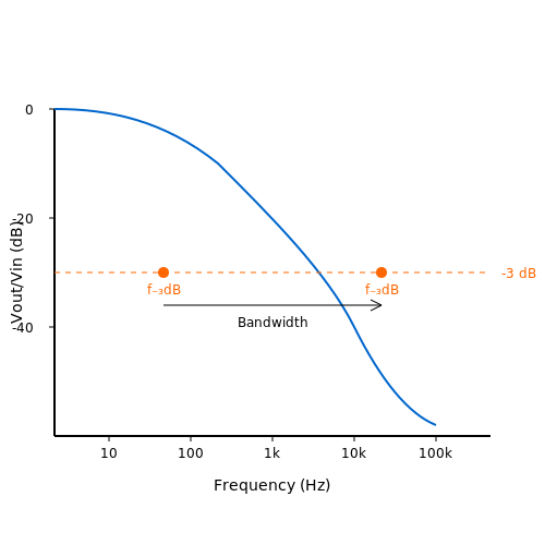
Multisim serves as a powerful tool for designing and prototyping electronic circuits before physical implementation. Engineers leverage its SPICE-based simulation engine to model complex analog, digital, and mixed-signal circuits with high accuracy. The software enables parametric sweeps of components (e.g., resistors, capacitors, active devices) to optimize performance metrics such as gain, bandwidth, and power dissipation. For instance, a common-emitter amplifier's frequency response can be simulated by sweeping capacitance values while observing Bode plots in real time.
Power Electronics Analysis
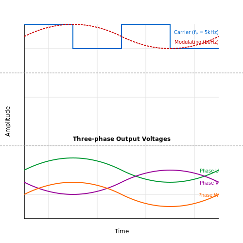
In power electronics, Multisim facilitates the analysis of switch-mode converters (buck, boost, flyback) and motor drive circuits. Users can simulate PWM-controlled systems with realistic semiconductor models, including MOSFETs and IGBTs with nonlinear junction capacitances. Thermal effects are incorporated through loss calculations based on device datasheet parameters. A typical application involves simulating a three-phase inverter's output voltage harmonics under varying load conditions:
RF and Microwave Circuit Simulation
The software's RF module supports S-parameter analysis up to GHz frequencies, enabling the design of impedance-matching networks and filter structures. Smith chart utilities allow for interactive transmission line tuning, while noise figure calculations predict receiver sensitivity. A practical case involves optimizing a low-noise amplifier's stability factor (k) through stability circles plotted directly from simulated Y-parameters.
Digital Logic Verification
For digital systems, Multisim integrates HDL co-simulation with VHDL/Verilog components alongside analog circuitry. This hybrid capability is critical for validating mixed-signal ASICs or FPGA interfaces. Engineers can test state machine logic under worst-case timing conditions by injecting jitter and propagation delays derived from IBIS models.
Educational and Research Applications
In academia, Multisim bridges theoretical concepts with practical observations through virtual laboratories. Graduate researchers employ its Monte Carlo analysis to study component tolerance effects on circuit yield, while its integration with LabVIEW enables hardware-in-the-loop validation. A notable example includes simulating memristor-based neuromorphic circuits to analyze their spike-timing-dependent plasticity characteristics.
Automated Test Scenario Generation
The software's test automation interface (TAI) allows scripting of complex test sequences using Python or .NET. This feature is extensively used in production testing environments to validate power supply units under dynamic load transients, with results exported directly to LIMS systems for statistical process control.
2. Installing and Setting Up Multisim
Installing and Setting Up Multisim
System Requirements
Before installing Multisim, ensure your system meets the minimum hardware and software requirements:
- Operating System: Windows 10 or 11 (64-bit). Earlier versions may lack driver support.
- Processor: Intel Core i5 or equivalent, with a clock speed ≥ 2.5 GHz.
- RAM: Minimum 8 GB (16 GB recommended for large simulations).
- Disk Space: 10 GB free space for installation, plus additional space for project files.
- Graphics: DirectX 11 compatible GPU with 1 GB VRAM.
Verify that your system has administrative privileges and that all pending Windows updates are installed to avoid compatibility issues.
Downloading Multisim
Multisim is available through NI (National Instruments) or authorized distributors. Follow these steps:
- Visit the NI Multisim download page.
- Select the version matching your license (Student, Professional, or Power Pro).
- Download the offline installer if internet connectivity is unreliable.
For academic users, ensure your institution provides a valid license file (.lic) or serial number.
Installation Process
The installation involves several critical steps:
- Run the Installer: Execute NI_Circuit_Design_Suite_XX.exe (where XX denotes the version).
- License Agreement: Accept NI’s terms and select Custom Installation to enable SPICE-specific components.
- Component Selection: Ensure the following are checked:
- Multisim Core
- NI Ultiboard (for PCB design integration)
- SPICE Simulation Engines (e.g., XSPICE, VHDL co-simulation)
- Installation Path: Avoid system directories (e.g., C:\Program Files) to prevent permission conflicts.
- Driver Installation: Allow the installer to deploy NI-VISA and NI-DAQmx drivers if interfacing with hardware.
Post-installation, reboot the system to finalize driver integration.
Initial Configuration
Launch Multisim and configure the environment for optimal performance:
- Workspace Layout: Navigate to Options > Global Preferences and set:
- SPICE solver to Modified Nodal Analysis (MNA) for nonlinear circuits.
- Default simulation temperature to 27°C (300 K) for consistency with SPICE defaults.
- Library Management: Add custom component libraries via Tools > Database > Database Manager.
- Simulation Settings: Under Simulate > Interactive Simulation Settings, adjust:
- Time step to 1e-6 s for transient analysis.
- Relative tolerance (RELTO) to 0.001 for high-precision circuits.
License Activation
For commercial licenses, activate using one of these methods:
- Serial Number: Enter the 24-digit code in NI License Manager.
- License File: Import the .lic file provided by NI.
- Cloud Licensing: Link to an NI account for floating licenses.
If activation fails, verify firewall exceptions for NI License Manager (port 1800).
Verifying the Installation
Confirm successful setup by simulating a test circuit:
- Create a simple RC low-pass filter (1 kΩ resistor, 1 µF capacitor).
- Run a transient analysis with a 1 V square wave input (1 kHz).
- Check the output waveform for an exponential decay (time constant τ = RC = 1 ms).
If the simulation diverges or crashes, reinstall the SPICE engine via NI Package Manager.
Common Issues and Troubleshooting
- Missing Components: Reinstall the Master Database from NI Update Service.
- Simulation Errors: Adjust solver settings or reduce circuit complexity.
- Performance Lag: Disable real-time anti-virus scanning for Multisim processes.
Navigating the Multisim Interface
Workspace Layout
The Multisim interface is organized into several key functional areas, each serving a distinct purpose in the circuit design and simulation workflow. The Design Toolbar provides quick access to schematic capture tools, while the Simulation Toolbar contains controls for running and analyzing simulations. The central Workspace is where circuits are constructed, flanked by the Component Browser on the left and the Instruments Palette on the right.
Component Management
Multisim's Component Browser uses a hierarchical database structure, with components organized by type (e.g., Basic, Transistors, ICs). The search functionality supports both parametric filtering and keyword matching. When placing components, right-click context menus provide access to advanced properties such as:
- SPICE model parameters
- Temperature coefficients
- Component tolerances
Schematic Capture Tools
The Wiring Tool automatically creates optimized connections with minimal crossings. For complex designs, the Bus Tool allows grouping of related signals. Advanced users can utilize:
Instrumentation Panel
Virtual instruments in Multisim provide real-time measurement capabilities comparable to physical lab equipment. The Oscilloscope interface includes:
- Adjustable timebase (1ns/div to 1000s/div)
- Voltage ranges from 1μV/div to 1kV/div
- FFT analysis up to 10MHz bandwidth
Simulation Controls
The Interactive Simulation mode allows real-time parameter tweaking, while Parameter Sweep automates analysis across component values. For power electronics, the Power Probes feature calculates:
Advanced Navigation Features
Keyboard shortcuts significantly enhance workflow efficiency:
| Shortcut | Function |
|---|---|
| Ctrl+Space | Component quick search |
| Alt+G | Toggle grid visibility |
| Ctrl+Shift+A | Advanced simulation settings |
Customization Options
Power users can modify the interface through View > Toolbars > Customize, creating personalized workspaces for specific applications like RF design or power electronics. The Color Scheme Editor allows adjustment of schematic aesthetics for improved readability in complex designs.
2.3 Creating a New Project
Project Initialization and Configuration
To begin a new simulation in Multisim, launch the software and select File → New → Project. A dialog box appears, prompting the user to define the project type, name, and location. For advanced users, the critical choices are:
- Analog/Digital Mixed-Signal Project: Enables SPICE-based simulation with mixed-signal components.
- RF Project: Optimized for high-frequency circuit analysis with S-parameter support.
- MCU Co-Simulation Project: Integrates microcontroller emulation for embedded system design.
The default SPICE solver settings are sufficient for most applications, but engineers working with nonlinear circuits may need to adjust the Gmin stepping algorithm or absolute tolerance parameters under Simulate → Interactive Simulation Settings.
Schematic Capture and Hierarchy
Multisim employs a hierarchical design structure. The top-level schematic (Main) can reference subcircuits through Hierarchical Blocks. To create a reusable subcircuit:
- Right-click on the workspace and select Place → Hierarchical Block.
- Define input/output pins using Place → Connectors.
- Double-click the block to edit its internal schematic.
This modular approach is particularly useful for large systems like phased-array antennas or multi-stage amplifiers, where individual components require isolated testing.
Netlist Generation and SPICE Integration
Behind the GUI, Multisim generates a SPICE netlist for simulation. The netlist structure follows:
* Multisim Netlist Example
V1 1 0 DC 5
R1 1 2 1k
C1 2 0 1u
.tran 1u 10m
.end
Advanced users can directly edit the netlist via Tools → Netlist Viewer, which is essential when implementing custom SPICE models or modifying convergence parameters.
Custom Component Integration
For components not in the default library:
where \(I_S\) is saturation current and \(n\) is the ideality factor. To implement this diode model:
- Navigate to Tools → Component Wizard.
- Select SPICE Model and input the governing equations.
- Define footprint and symbol mapping for PCB integration.
Version Control and Collaboration
Multisim supports Git integration through the Team Design feature. To enable:
- Configure repository path under Options → Version Control.
- Use Design → Push/Pull for synchronization.
- Conflict resolution follows standard diff tools for
.ms14files.
3. Adding Components to the Workspace
Adding Components to the Workspace
Multisim’s component library is organized hierarchically, allowing users to access a vast array of electronic components, from passive elements like resistors and capacitors to active devices such as transistors and integrated circuits. Components are grouped by functionality and manufacturer, ensuring efficient retrieval for both theoretical and practical circuit design.
Accessing the Component Database
The component database is accessed via the Place Component dialog (Ctrl+W). This dialog provides a searchable interface with filters for component type, manufacturer, and footprint. Advanced users can leverage the Database Manager to add custom components or modify existing ones, ensuring accurate simulation parameters.
Placing Components on the Workspace
Once a component is selected, it appears as a floating symbol attached to the cursor. Left-clicking places the component, while right-clicking rotates it in 90° increments. Holding Ctrl during placement creates multiple instances, streamlining the design of repetitive circuits like filters or amplifiers.
Parameter Customization
Double-clicking a placed component opens its properties panel, where advanced parameters such as tolerance, temperature coefficients, and SPICE models can be adjusted. For semiconductor devices, the Edit Model button provides access to nonlinear parameters like beta (β) for BJTs or threshold voltage (Vth) for MOSFETs.
Wiring Components
Components are interconnected using the Wire Tool (Ctrl+Shift+W). Multisim automatically snaps wires to component terminals, ensuring clean connections. For high-frequency or precision analog circuits, controlled impedance routing can be enabled in the PCB Layout settings.
Hierarchical Blocks and Subcircuits
Complex designs benefit from hierarchical blocks, which encapsulate subcircuits into reusable modules. These blocks can be defined using the Place Hierarchical Block option, with internal circuitry edited via a double-click. This is particularly useful for modular designs like multi-stage amplifiers or digital systems.
* Example SPICE Subcircuit Definition
.subckt OPAMP 1 2 3
R1 1 2 1MEG
R2 2 3 10K
E1 3 0 1 2 1E6
.ends
3.2 Wiring Components Together
Wiring components in Multisim involves establishing electrical connections between terminals while adhering to Kirchhoff's laws and ensuring signal integrity. Unlike breadboarding, virtual wiring eliminates parasitic effects but requires precise topology definition for accurate simulation.
Connection Rules and Constraints
Multisim enforces strict connectivity rules:
- Unconnected pins trigger simulation errors unless explicitly flagged as no-connect (NC).
- Floating nets automatically assume infinite impedance, potentially causing convergence issues.
- Crossing wires without junctions remain unconnected—junctions must be explicitly placed.
The software performs real-time design rule checking (DRC) during wiring operations, preventing:
- Direct voltage source shorts (zero-resistance paths)
- Invalid ground loops
- Unterminated transmission lines
Wire Routing Algorithms
Multisim employs modified Lee's algorithm for auto-routing, minimizing:
where Ltotal represents the cumulative Manhattan distance between component pins. The router prioritizes:
- Minimizing parallel runs with high dV/dt signals
- Avoiding 90° bends for RF circuits
- Maintaining clearance from high-impedance nodes
Net Naming Conventions
Critical nets should be explicitly labeled to facilitate:
- Probing during interactive simulation
- Cross-referencing in Bill of Materials (BOM)
- Hierarchical design navigation
Net naming follows SPICE conventions—special characters like brackets [] denote bus members, while underscores _ separate hierarchical blocks.
Advanced Wiring Techniques
Differential Pair Routing
For high-speed designs, maintain:
where c is light speed and ϵr is substrate permittivity. Use the Differential Pair Designer tool to:
- Match trace lengths
- Set controlled impedance
- Define coupling coefficients
Power Distribution Networks
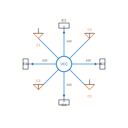
Implement star topologies for low-noise power delivery:
Key considerations include:
- Decoupling capacitor placement within λ/20 of IC pins
- Separate analog/digital ground pours
- Current density verification via thermal analysis
Signal Integrity Verification
After wiring completion, run pre-simulation checks:
- Continuity testing via net highlight mode
- Crosstalk analysis using field solver integration
- Propagation delay estimation through transmission line models
The Signal Integrity Analyzer calculates eye diagrams and bit error rates based on:
where σn represents accumulated noise from all coupled nets.
3.3 Running a Basic Simulation
Initializing the Simulation Environment
Before executing a simulation in Multisim, ensure the circuit schematic is correctly constructed with all necessary components, proper connections, and appropriate ground references. Navigate to the Simulate menu and select Analyses and Simulation. Multisim supports various simulation types, including transient, AC sweep, DC operating point, and Fourier analysis. For a basic simulation, the Interactive Simulation mode provides real-time feedback, while Single Frequency AC Analysis or Transient Analysis offers deeper insights into circuit behavior.
Configuring Simulation Parameters
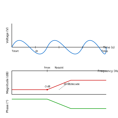
For a transient analysis, define the Start Time (Tstart), End Time (Tstop), and Time Step (Δt). The Nyquist criterion must be satisfied to avoid aliasing, ensuring the sampling rate is at least twice the highest frequency component. For example, simulating a 1 kHz sine wave requires:
In AC sweep analysis, specify the frequency range (e.g., 10 Hz to 100 MHz) and sweep type (linear or logarithmic). Multisim internally employs SPICE algorithms, leveraging nodal analysis to solve Kirchhoff’s current law (KCL) equations:
Running the Simulation
Click Run to initiate the simulation. Multisim dynamically solves the circuit matrix using modified nodal analysis (MNA), accounting for nonlinear components like diodes and transistors via Newton-Raphson iteration. The simulation engine first computes the DC operating point before proceeding with transient or AC analysis. For circuits with oscillators or feedback loops, enable UIC (Use Initial Conditions) to bypass the DC analysis phase.
Interpreting Results
Output waveforms appear in the Grapher View. For transient simulations, voltage and current traces are plotted against time. In AC analysis, magnitude (dB) and phase (degrees) are displayed on a Bode plot. Right-click any trace to perform measurements (e.g., RMS, peak-to-peak, rise time). For noise analysis, Multisim calculates equivalent input noise density:
where k is Boltzmann’s constant, T is temperature, R is resistance, and Δf is bandwidth.
Debugging Common Issues
If the simulation fails to converge, check for:
- Floating nodes (ensure all components are grounded or referenced).
- Unrealistic component values (e.g., 1 TΩ resistors).
- Conflicting initial conditions in energy-storage elements (capacitors/inductors).
Adjust the SPICE Tolerance settings under Simulate > Interactive Simulation Settings to relax convergence criteria if necessary.
Advanced Features
For RF circuits, enable RF Mode to account for transmission line effects. Coupled with parameter sweeps, Multisim can optimize component values against user-defined goals (e.g., maximize gain, minimize distortion). Export simulation data to MATLAB or Excel for post-processing using the Export to MathScript feature.
3.4 Analyzing Simulation Results
Multisim provides a suite of powerful tools for analyzing simulation results, enabling engineers to extract meaningful insights from circuit behavior. The post-simulation phase involves interpreting waveforms, validating theoretical predictions, and diagnosing anomalies.
Time-Domain and Frequency-Domain Analysis
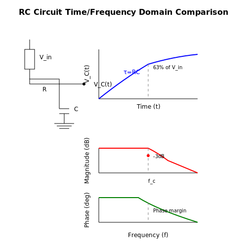
Transient analysis yields time-domain waveforms, where voltage and current are plotted against time. For a simple RC circuit, the capacitor voltage VC(t) follows:
Frequency-domain analysis, such as AC Sweep, reveals the circuit's response across a range of frequencies. The transfer function H(f) of a low-pass filter is:
Bode plots generated from this data show magnitude (in dB) and phase shift, critical for stability analysis in feedback systems.
Parametric Sweeps and Monte Carlo Analysis
Parametric sweeps evaluate circuit performance across component values. For instance, varying resistance R in a voltage divider:
Monte Carlo simulations introduce statistical variations in components (e.g., ±5% tolerance). The resulting histograms quantify yield rates and sensitivity to manufacturing deviations.
Advanced Visualization Tools
- Cursor Measurements: Precise extraction of peak values, rise times, and settling times from waveforms.
- FFT (Fast Fourier Transform): Identifies harmonic distortion in nonlinear circuits.
- Eye Diagrams: Assess signal integrity in high-speed digital designs.
Exporting Data for Further Processing
Multisim allows exporting raw data to MATLAB or Python for custom analysis. A typical workflow involves:
import numpy as np
import matplotlib.pyplot as plt

# Load exported Multisim data
time, voltage = np.loadtxt('transient_analysis.csv', delimiter=',', unpack=True)

# Plot results
plt.plot(time, voltage)
plt.xlabel('Time (s)')
plt.ylabel('Voltage (V)')
plt.grid(True)
plt.show()
For power electronics, efficiency η is calculated from exported current and voltage:
Debugging Common Simulation Errors
Convergence failures often stem from:
- Abrupt changes in nonlinear components (e.g., diodes, transistors).
- Insufficient time-step resolution in transient analysis.
- Floating nodes or incorrect ground references.
Adjusting solver settings (e.g., Gear method for stiff systems) or adding parallel resistors (1 GΩ) to floating nodes typically resolves these issues.
4. Using Virtual Instruments
4.1 Using Virtual Instruments
Virtual Instrumentation in Multisim
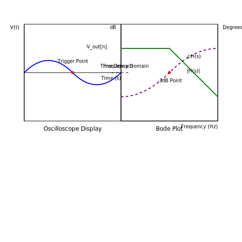
Multisim integrates a suite of virtual instruments that emulate real-world laboratory equipment, enabling precise circuit analysis without physical hardware. These instruments interface with the schematic environment through dynamic probes, allowing real-time measurement of voltage, current, frequency, and other parameters. The instruments are categorized into:
- Oscilloscopes (e.g., Tektronix 4-channel)
- Function Generators (arbitrary waveform support)
- Bode Plotters (frequency response analysis)
- Logic Analyzers (digital signal capture)
Oscilloscope Implementation
The oscilloscope’s time-domain analysis relies on Kirchhoff’s laws and numerical integration. For a voltage signal V(t) sampled at intervals Δt, the displayed waveform is computed using:
where N is the FFT window size. Multisim’s oscilloscope supports:
- Bandwidth up to 1 GHz (simulated)
- Trigger modes: edge, pulse, and pattern
- Math channels for differential measurements
Bode Plotter for Frequency Analysis
The Bode plotter automates AC sweep analysis by solving the circuit’s transfer function H(s) across a user-defined frequency range. For a second-order low-pass filter:
Key configuration parameters include:
- Start/stop frequency (1 mHz to 10 THz)
- Points per decade (logarithmic scaling)
- Reference impedance (default 50Ω)
Logic Analyzer for Digital Circuits
Captures digital signals with timing resolution down to 10 ps. The analyzer decodes bus transactions using:
Supports protocols like I²C, SPI, and UART through protocol decoders. Timing violations are flagged using configurable thresholds.
Practical Considerations
Virtual instruments introduce simulation artifacts not present in physical hardware:
- Quantization noise from finite numerical precision
- Time-step aliasing in transient analysis
- Non-ideal probe loading effects (1 MΩ || 20 pF default)
Calibration procedures mirror real instruments—for example, the oscilloscope’s vertical scale requires adjustment when measuring high-impedance nodes to account for current leakage.
Parameter Sweep Analysis
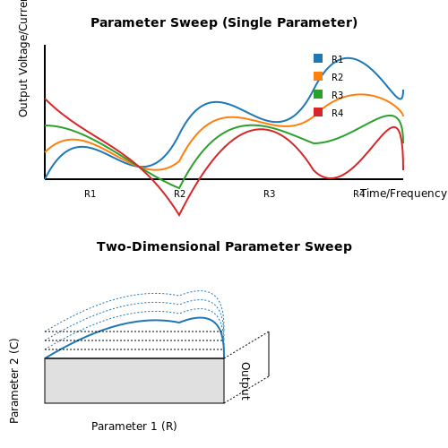
Parameter Sweep Analysis in Multisim allows engineers to evaluate circuit performance across a range of component values, operating conditions, or model parameters. This technique is indispensable for sensitivity analysis, optimization, and robustness testing in analog and mixed-signal designs.
Mathematical Foundation
The core principle involves solving the circuit equations iteratively while varying one or more parameters. For a linear time-invariant (LTI) system with a transfer function H(s), the output response Y(s) to an input X(s) becomes:
where p represents the swept parameter. The DC operating point is recalculated for each parameter value using modified nodal analysis:
with G being the conductance matrix and V the node voltage vector.
Implementation in Multisim
To configure a parameter sweep:
- Navigate to Simulate → Analyses → Parameter Sweep
- Select the target component parameter (resistance, capacitance, etc.)
- Define the sweep type:
- Linear: Uniform steps between start and end values
- Decade: Logarithmic steps per decade
- Octave: Doubling/halving steps
- List: User-specified discrete values
- Set the analysis type to run at each point (DC, AC, transient)
Advanced Applications
Monte Carlo Analysis
When combined with statistical distributions, parameter sweep becomes Monte Carlo analysis. For a resistor with 5% tolerance:
Temperature Dependence
Semiconductor parameters often follow Arrhenius-like temperature dependence:
where Eg is the bandgap energy and k Boltzmann's constant.
Visualization Techniques
Multisim provides several ways to analyze sweep results:
- Family of curves: Overlaid plots for different parameter values
- 3D surfaces: For two-dimensional parameter sweeps
- Performance graphs: Metrics like bandwidth vs. component value
* Sample SPICE directive for parameter sweep
.DC PARAM Rval 1k 10k 0.5k
R1 1 2 {Rval}
Practical Considerations
For circuits with high parameter sensitivity, adaptive step sizing improves efficiency:
where α controls the adaptation rate. Convergence issues can be mitigated by:
- Setting appropriate relative tolerances (RELTOL)
- Using Gmin stepping algorithms
- Implementing continuation methods for strongly nonlinear systems
4.3 Monte Carlo Analysis
Fundamentals of Monte Carlo Simulation
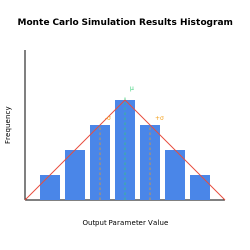
Monte Carlo analysis is a statistical method used to assess the impact of component tolerances on circuit performance. By repeatedly sampling component values from predefined statistical distributions (e.g., Gaussian or uniform), it generates a probabilistic output response. In Multisim, this technique evaluates how manufacturing variations affect key parameters like gain, bandwidth, or power dissipation.
where N is the number of iterations, and f(Ri, Ci, βi) represents the circuit's transfer function with randomized parameters.
Implementation in Multisim
To configure a Monte Carlo analysis in Multisim:
- Define tolerance models for components (e.g., resistors ±5%, capacitors ±10%)
- Specify the number of runs (typically 100–10,000 for convergence)
- Select output variables (e.g., node voltages, branch currents)
- Choose distribution type: Gaussian (3σ limits) or Uniform
Statistical Output Interpretation
Multisim generates histograms and statistical metrics:
Critical outputs include yield analysis (percentage of runs meeting specs) and sensitivity rankings.
Practical Considerations
Convergence testing is essential—increase iterations until mean and standard deviation stabilize. For nonlinear circuits, 10,000+ runs may be needed. Multisim's batch mode allows distributed computing to accelerate large-scale analyses.
Advanced Applications
Combined with temperature sweeps or corner analysis, Monte Carlo simulations predict worst-case scenarios for mission-critical systems. Aerospace and medical device designs often require 6σ (99.99966% yield) verification through this method.
* Sample Monte Carlo Netlist for Multisim
.MC 1000 DC V(OUT) LIST
+ R1(R=1k DEV=5%)
+ C1(C=10n DEV=10%)
+ Q1(BF=100 DEV=20%)
Temperature and Noise Analysis
Temperature Analysis in Multisim
Temperature effects in electronic circuits are modeled in Multisim using temperature-dependent device parameters derived from semiconductor physics. The simulator adjusts component values based on the specified temperature sweep range, typically from -55°C to 125°C for industrial applications. For a bipolar junction transistor, the temperature-dependent collector current is given by:
where the thermal voltage VT varies with temperature:
Multisim implements the Gummel-Poon model for BJTs and BSIM models for MOSFETs, both incorporating temperature coefficients for accurate simulation. The temperature analysis tool performs a DC sweep while recomputing all device parameters at each temperature point, revealing critical thermal dependencies in bias points and gain characteristics.
Noise Analysis Methodology
Multisim's noise analysis computes the equivalent input noise density and output noise spectrum using nodal analysis with noise sources. For each resistor, the thermal noise is modeled as:
Semiconductor devices contribute shot noise and flicker noise components:
The simulator constructs a noise correlation matrix and solves for the transfer function from each noise source to the output, then refers all contributions back to the input as an equivalent noise voltage or current. This enables calculation of the signal-to-noise ratio (SNR) and noise figure (NF) across the specified frequency range.
Practical Implementation
To perform combined temperature-noise analysis:
- Define the temperature sweep range in the simulation profile
- Enable noise analysis with appropriate output and reference nodes
- Set the frequency sweep parameters matching the circuit's operational bandwidth
- Specify device temperature coefficients when available
The results reveal critical thermal-noise tradeoffs, such as the degradation of amplifier noise performance at elevated temperatures due to increased leakage currents and reduced carrier mobility. In RF circuits, temperature-induced impedance mismatches can significantly alter noise matching conditions.
Advanced Considerations
For accurate high-frequency noise analysis, Multisim incorporates:
- Parasitic-aware models of component packaging
- Substrate noise coupling effects in IC designs
- Non-quasi-static transistor noise models
- Correlated noise sources in differential pairs
The simulator's advanced algorithms handle noise-temperature cross-correlation effects, particularly important in low-noise amplifiers and precision analog circuits where thermal drift modulates noise characteristics. Users can export the complete noise covariance matrix for further statistical processing.
5. Common Simulation Errors and Fixes
5.1 Common Simulation Errors and Fixes
Convergence Failures in Nonlinear Circuits
Convergence failures occur when the solver cannot find a stable operating point for nonlinear components like diodes, transistors, or op-amps. Multisim uses the Newton-Raphson iterative method, which may fail if:
- The initial guess is too far from the solution.
- The circuit contains discontinuities (e.g., ideal switches).
- Component models have sharp transitions (e.g., Zener diodes near breakdown).
To resolve this, adjust the SPICE Options:
Modify RELTOL (default: 0.001) or GMIN (default: 1e-12) to improve convergence. For example:
.options RELTOL=0.01 GMIN=1e-9
Grounding and Floating Node Errors
Floating nodes arise when components lack a DC path to ground, causing singular matrix errors. For instance, capacitors or transformers without parallel resistors create high-impedance nodes. Add a high-value resistor (e.g., 1 GΩ) to ground:
Time Step Too Small Errors
This error occurs when the simulation step size becomes smaller than the solver’s minimum threshold, often due to:
- Fast-switching signals (e.g., PWM with nanosecond edges).
- Stiff systems with mixed time constants (e.g., LC filters with parasitic Rs).
Increase ITL4 (default: 10) or use UIC (Skip Initial Operating Point):
.tran 1us 1ms UIC
.options ITL4=100
Model Parameter Mismatches
Incorrect SPICE model parameters (e.g., BV=100 for a 5V Zener diode) cause unrealistic behavior. Verify model libraries and override parameters:
.model DZENER D(Is=1e-14 BV=5.1 IBV=1e-3)
Singular Matrix Errors
A singular matrix indicates a topological issue, such as:
- Voltage sources in parallel without series resistance.
- Loops of inductors or capacitors without damping.
Add series resistors (e.g., 1 mΩ for inductors) or parallel resistors (e.g., 1 MΩ for capacitors).
5.2 Optimizing Simulation Performance
Parallel Processing and Solver Selection
Multisim leverages parallel processing to accelerate simulations, particularly for large-scale circuits. The default Modified Nodal Analysis (MNA) solver is efficient for most analog circuits, but switching to the SPARSE solver can reduce computation time for circuits with high node counts (>10,000). Enable parallel processing via:
Simulate > Interactive Simulation Settings > Solver > Enable Parallel ProcessingThe computational complexity of MNA is given by:
where n is the number of nodes. For RF circuits, the Harmonic Balance solver offers better convergence for periodic steady-state analysis.
Time-Step Optimization
Adaptive time-stepping reduces unnecessary computations. The local truncation error (LTE) constraint is:
where ϵ is the relative tolerance (default: 1e-3) and h is the step size. Adjust tolerances via:
Simulate > Analyses and Simulation > Transient > Advanced > Custom TolerancesFor switching circuits, enforce a maximum step size of 1/100th of the smallest switching period to capture transients accurately.
Model Simplification
Replace nonlinear components with behavioral models (e.g., VCOs with ideal sine sources) where possible. The simulation time for a MOSFET scales as:
where Niter is Newton-Raphson iterations and Cdevice is the device complexity. Use ideal switches instead of transistors for digital control logic.
Frequency Domain Techniques
For AC analysis, enable Fast Fourier Transform (FFT) compression to reduce memory usage. The Nyquist criterion must be satisfied:
where fmax is the highest frequency of interest. Multisim’s Smart Simulation mode automatically decimates low-bandwidth signals.
Hardware Acceleration
GPU offloading is available for:
- Monte Carlo analyses (parallelizable trials)
- Parametric sweeps (independent runs)
- Convolution-based RF simulations (CUDA-optimized)
Enable via Tools > Options > GPU Acceleration. Benchmark tests show a 3–8× speedup for circuits with >500 reactive components.
Cache Management
Multisim caches previous simulation results to skip redundant calculations. The cache size (default: 2GB) can be adjusted in:
Tools > Options > Circuit > Simulation CacheFor multi-day simulations, enable Periodic Save to prevent data loss. The checkpoint interval should be ≤10% of total expected runtime.
5.3 Debugging Circuits in Multisim
Common Debugging Challenges in Multisim
Debugging circuits in Multisim requires a systematic approach to identify and resolve issues such as incorrect component values, improper connections, or simulation errors. Advanced users must be familiar with Multisim's diagnostic tools, including the Interactive Simulation mode, Probe functionality, and Error Log analysis.
One frequent issue arises from floating nodes—unconnected pins that introduce undefined states. Multisim flags these with a red dot, but deeper analysis may require probing node voltages or currents. Another common problem involves convergence errors in nonlinear circuits, often due to unrealistic initial conditions or conflicting parameter settings.
Using the Error Log and Simulation Diagnostics
Multisim's Error Log provides detailed feedback when simulations fail. For example, a transient analysis might fail with the message: "Time step too small". This typically indicates stiff differential equations, which can be mitigated by adjusting the Maximum Time Step in the simulation settings or modifying circuit damping.
If the error persists, enabling the SPICE Netlist debug option allows inspection of the underlying nodal equations. The netlist reveals how Multisim interprets the circuit topology, helping identify misplaced grounds or incorrect component models.
Probing Signals and Dynamic Analysis
Multisim's Probe tool provides real-time measurement of voltages, currents, and power dissipation. For AC analysis, the Bode Plotter and Oscilloscope instruments visualize frequency response and transient behavior. When probing high-frequency circuits, ensure the simulation step size is sufficiently small to capture signal dynamics:
where fmax is the highest frequency of interest. Incorrect step sizes lead to aliasing or inaccurate rise/fall times in digital circuits.
Convergence and Solver Settings
Nonlinear circuits (e.g., oscillators, PLLs) often require tweaking solver parameters. The Gmin Stepping algorithm helps bypass convergence failures by gradually increasing conductance between nodes. Adjusting RELTOL (relative tolerance) and ABSTOL (absolute tolerance) can also stabilize simulations:
For circuits with feedback loops, enabling UIC (Use Initial Conditions) skips the DC operating point calculation, which may otherwise diverge.
Case Study: Debugging an Active Filter
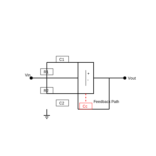
Consider a Sallen-Key bandpass filter exhibiting unexpected gain peaking. The AC Analysis shows instability at the cutoff frequency. Probing the op-amp's output reveals oscillation due to insufficient phase margin. Modifying the feedback network's resistor values or adding a compensation capacitor resolves the issue, verified by re-running the Parameter Sweep tool.
6. Recommended Books and Manuals
6.1 Recommended Books and Manuals
- Using Multisim 6.1: Amazon.co.uk: Reeder QC, John: 9780766811331: Books — Buy Using Multisim 6.1 by Reeder QC, John (ISBN: 9780766811331) from Amazon's Book Store. Everyday low prices and free delivery on eligible orders.
- PDF Electronics Communication Simulation Lab Manual Us [PDF] — Roy Blake Electronics Communication Simulation Lab Manual Us: Handbook of Laboratory Experiments in Electronics and Communication Engineering A M Zungeru,J M Chuma,M Mangwala,L K Ketshabetswe,2017-03-08 This Handbook is prepared after extensive simulations of circuits with some electronic and engineering software such as Multisim Pspice Proteus MATLAB and Circuit Logic The Handbook is designed ...
- PDF Electronics Circuits Lab Manual Using Multisim (book) — John Okyere Attia Electronics Circuits Lab Manual Using Multisim: Multisim Experiments for DC/AC, Digital, and Devices Courses Gary Snyder,David M. Buchla,2011 The National Instruments Multisim software is a versatile design and simulation program The intent of this workbook is to simulate a laboratory experience in electronics and help you develop a working knowledge of the Multisim software ...
- PDF Digital Electronics Principles And Applications Experiments W Multisim — Digital electronics is a fundamental field in modern technology, powering everything from smartphones and computers to industrial automation and medical devices. Understanding its principles and applications is essential for aspiring engineers, technicians, and hobbyists alike. Multisim, a user-friendly simulation software, offers a powerful platform for learning and experimenting with digital ...
- Using Multisim 6.1 Troubleshooting DC/AC Circuits - amazon.com — This unique workbook teaches how to troubleshoot circuits with the help MultiSIM (TM) 6.1. Working on the computer, you will learn to make measurements, replace components, and test results just as you would in a lab. Circuits contain built-in faults to give you troubleshooting practice.
- Using Multisim 6.1: Troubleshooting DC/AC Circuits (Book Only): Reeder ... — This unique workbook teaches how to troubleshoot circuits with the help MultiSIM (TM) 6.1. Working on the computer, you will learn to make measurements, replace components, and test results just as you would in a lab. Circuits contain built-in faults to give you troubleshooting practice.
- Amazon.com: Multisim — Simulation-based Labs for Circuit Analysis: Discovering Circuits with Multisim Live and Tinkercad (River Publishers Series in Electronic Materials, Circuits and Devices)
- PDF Archived: Multisim User Guide - National Instruments — Multisim is the schematic capture and simulation application of National Instruments Circuit Design Suite, a suite of EDA (Electronics Design Automation) tools that assists you in carrying out the major steps in the circuit design flow.
- PDF Laboratory Manual Electrical Circuits and Simulation - Aurora — By this perspective we have introduced a Laboratory manual cum Observation for Electrical Circuits and Simulation.
- PDF ELECTRICAL Engineering department - PTSB — ell as all the lecturers involve. It provides guidance for students to do their practical lab by using multisim online simulator. There are 6 chapters covered in this e-book which is Bridge Rectifier Circuit, Oscillator, Operational Amplifier, Astable Multivibrator, Filter and Analog to Digital or Digital to Analog Converter. In this e- book will present valuable information with supporting ...
6.2 Online Resources and Tutorials
- 6.2 - Multisim Live — NI Multisim Live lets you create, share, collaborate, and discover circuits and electronics online with SPICE simulation included ... Resources. Get Started Help Idea ... NI Multisim Live lets you create, share, collaborate, and discover circuits and electronics online with SPICE simulation included Browser not supported Safari version 15 and ...
- 6.2 - Practice - Multisim Live — NI Multisim Live lets you create, share, collaborate, and discover circuits and electronics online with SPICE simulation included ... Resources. Get Started Help Idea Exchange Support Forum FAQ. ... share, collaborate, and discover circuits and electronics online with SPICE simulation included Browser not supported Safari version 15 and newer ...
- PDF EE100 MultiSim Tutorial - University of California, Berkeley — Circuit simulation with SPICE (and MultiSim) involves two steps: (1) Enter in the circuit schematic (with MultiSim's graphical user interface). (2) Choose the type of analysis and run the simulation. 2. Organization of this Tutorial 1. Introduction 2. Organization I Basic Circuit Simulation Techniques in MultiSim 3. MultiSim Environment 4.
- Multisim Live Online Circuit Simulator — Multisim Live is a free, online circuit simulator that includes SPICE software, which lets you create, learn and share circuits and electronics online.
- NI myDAQ and NI Multisim Problems for Circuits Textbook — This supplement to Circuits by Ulaby, Maharbiz, and Furse (no longer available) contains 40 additional homework problems designed for three-way solutions: analytical, simulation, and measurement. After solving each problem analytically, the student continues by solving the same problem through simulation with NI Multisim (included with the textbook), and then once again through physical ...
- Electronic Circuits Workbook Using Multisim Online Simulator - ResearchGate — Electronic Circuits Workbook using multisim online simulator is special present for students who are studying Electronic Circuits course as well as all the lecturers involve.
- 2(1) - University of Michigan — Figure 6.2.4Analysis settings for the simulation. Transient . The output of the plot should resemble that shown in Fig. 6.2.5. As we can see the signal starts at 0 V (Initial Value = 0 V), and begins to rise immediately (Rise Delay Time = 0 ms) to 1V (Pulsed Value = 1V), with an exponential time constant of 0.001 s (Rise Time Constant = 1 ms).
- PDF ELECTRICAL Engineering department - PTSB — Electronic Circuits Workbook using multisim online simulator is our special present for students who are studying Electronic Circuits course as well as all the lecturers involve. It provides guidance for students to do their practical lab by using multisim online simulator. There are 6 chapters covered in this e-book
- Circuit Analysis and Design by Ulaby and Maharbiz - University of Michigan — A brief tutorial has been included for getting started with National Instruments Multisim TM software. As you will learn, Multisim is an extremely deep piece of software. While the textbook introduces many of Multisim's fundamental concepts, in the interest of space, many topics are also left out and those topics that are included are truncated.
- Practical Workbook Using Multisim Online Simulator - ResearchGate — PDF | Practical Lab for subject Electronic Circuits by using Multisim Online Simulator | Find, read and cite all the research you need on ResearchGate
6.3 Academic Papers and Case Studies
- Solved Consider the circuit shown in Figure L.6.3.2: FIGURE - Chegg — Engineering Electrical Engineering Electrical Engineering questions and answers Consider the circuit shown in Figure L.6.3.2: FIGURE L6.3.2: Circuit with diode-connected NPN transistor. Design the circuit in Figure L6.3.2 such that IC=1 mA and RE=15kΩ. Use supplies of V+=−V−=15 V. Use β=100 Hend calculations - Sketch the circuit in your lab book, clearly labeling the transistor's three ...
- Simulation of Electronic Circuits with Multisim™ - Springer — Previous chapter studied the simulation of electric circuits with Multisim. This chapter focus on the simulation of electronic circuits (i.e., circuits which contain diode, transistor, IC's, etc.) with Multisim.
- PDF Circuit Analysis with Multisim - ia902301.us.archive.org — ABSTRACT This book is concerned with circuit simulation using National Instruments Multisim. It focuses on the use and comprehension of the working techniques for electrical and electronic circuit simulation. The first chapters are devoted to basic circuit analysis.
- Wedge design for high-temperature ultrasonic flow rate measurement — Based on the Multisim simulation, reference the existing circuit knowledge, the specific circuit structure, model and parameters of the design nsor are shown in Figure 10. 5. Case Study and area. The voltage values measured by different materials are different, and the voltage values Figure 11. The developed eddy current sensor.
- (PDF) Circuit Simulation - Academia.edu — This paper discusses circuit simulation methodologies, focusing on the Gaussian elimination algorithm and various LU factorization techniques. Key implementations for forward and backward substitutions are presented based on matrix storage methods, alongside fundamental circuit simulation principles such as device equations and equation ...
- Circuit Analysis with Multisim by David Báez-López, Félix E. Guerrero ... — Circuit Analysis with Multisim Synthesis Lectures on Digital Circuits and Systems Editor Mitchell A. Thornton, Southern Methodist University The Synthesis Lectures on Digital Circuits and Systems series is comprised of 50- to 100-page books targeted for audience members with a wide-ranging background. The Lectures include topics that are of interest to students, professionals, and researchers ...
- Electronic Circuits Workbook Using Multisim Online Simulator - ResearchGate — Electronic Circuits Workbook using multisim online simulator is special present for students who are studying Electronic Circuits course as well as all the lecturers involve.
- Doering Mydaq Multisim-problems 3rd-Printing Optimized — Do all of this work on engineering green paper or in a lab book or as otherwise required by your instructor. The "Simulation" section presents your work to set up the circuit simu-lation in NI Multisim and the simusimu-lation results you used to obtain mean-ingful information.
- Practical Workbook Using Multisim Online Simulator - ResearchGate — PDF | Practical Lab for subject Electronic Circuits by using Multisim Online Simulator | Find, read and cite all the research you need on ResearchGate
- PDF ELECTRICAL Engineering department - PTSB — ell as all the lecturers involve. It provides guidance for students to do their practical lab by using multisim online simulator. There are 6 chapters covered in this e-book which is Bridge Rectifier Circuit, Oscillator, Operational Amplifier, Astable Multivibrator, Filter and Analog to Digital or Digital to Analog Converter. In this e- book will present valuable information with supporting ...