Bias Control in Synthetic Dataset Creation
1. Definition and Types of Bias in Data
Definition and Types of Bias in Data
Bias in data refers to systematic errors that skew the representation of the underlying population, leading to models that perpetuate or amplify these distortions. In synthetic dataset creation, controlling bias is critical to ensure fairness, generalizability, and robustness in downstream machine learning applications. Bias can manifest in multiple forms, each requiring distinct mitigation strategies.
Statistical Bias
Statistical bias arises when a dataset's statistical properties deviate from the true distribution of the target population. Common subtypes include:
- Sampling Bias: Occurs when data collection methods favor certain subgroups, leading to underrepresentation. For example, facial recognition datasets historically overrepresented lighter-skinned individuals, causing higher error rates for darker-skinned faces.
- Measurement Bias: Introduced by flawed instruments or inconsistent labeling protocols. In medical imaging, variations in scanner resolutions can artificially inflate diagnostic model performance.
- Selection Bias: Results from non-random exclusion of data points. A classic example is survey data omitting non-respondents, which may correlate with specific attitudes.
where \(\hat{\theta}\) is the estimator and \(\theta\) is the true population parameter. Minimizing this expectation is fundamental to unbiased synthetic data generation.
Societal Bias
Embedded cultural, gender, or racial prejudices in data reflect historical inequities. These biases often emerge through:
- Labeling Bias: Human annotators inject subjective judgments. A 2019 study revealed that sentiment analysis tools assigned more negative scores to texts containing African American Vernacular English (AAVE).
- Historical Bias: Pervasive structural inequalities in source data. Hiring datasets may replicate gender disparities in STEM fields if uncorrected.
Algorithmic Amplification
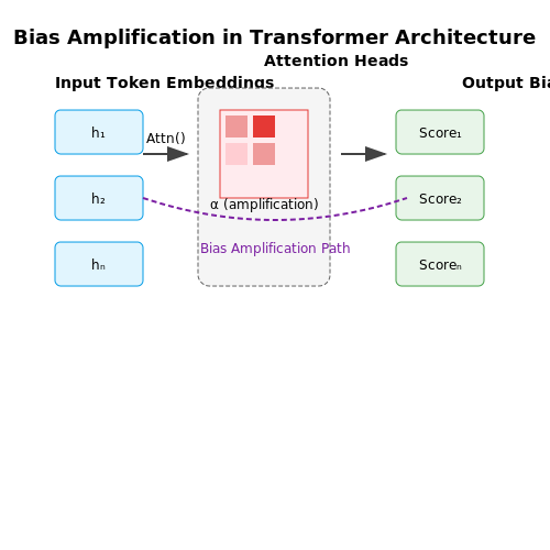
Machine learning models can exacerbate existing biases during synthetic data generation. For instance, generative adversarial networks (GANs) may over-sample majority classes if the loss function lacks fairness constraints. The amplification factor \(\alpha\) can be modeled as:
where values \(\alpha \gg 1\) indicate problematic reinforcement of biased patterns.
Temporal Bias
Datasets capturing dynamic systems may become outdated, causing concept drift. Financial fraud detection models trained on pre-2020 transaction data often fail to adapt to emerging cybercrime tactics. The decay rate \(\lambda\) of a feature's predictive power can be quantified as:
where AUC denotes model accuracy over time \(t\).
Geospatial Bias
Geographic imbalances affect models deployed across regions. Autonomous vehicle training data concentrated in urban areas performs poorly in rural environments. The spatial coverage gap \(\Delta_g\) between two regions \(A\) and \(B\) is:
with \(\Delta_g \rightarrow 1\) indicating severe disparity.
1.2 Sources of Bias in Synthetic Dataset Creation
Generative Model Biases
Synthetic datasets are often generated using deep generative models such as Generative Adversarial Networks (GANs) or Variational Autoencoders (VAEs). These models inherit biases present in their training data, which propagate into the synthetic outputs. For instance, if a GAN is trained on facial images with underrepresentation of certain ethnic groups, the generated faces will exhibit similar demographic skews. The bias can be quantified using statistical divergence measures between the real and synthetic distributions:
where DKL measures how much information is lost when Psyn approximates Preal. Non-zero values indicate distributional mismatch.
Sampling Strategy Biases
Even with unbiased generative models, improper sampling strategies introduce bias. Common issues include:
- Over-sampling frequent classes in imbalanced datasets, leading to overfitting.
- Under-sampling rare classes, causing loss of critical minority patterns.
- Non-random latent space traversal in VAEs, where linear interpolations may not map to semantically meaningful synthetic samples.
For example, stratified sampling that enforces equal class proportions may suppress naturally occurring frequency relationships needed for certain applications.
Feature Representation Biases
The choice of feature encoding schemes disproportionately affects synthetic data quality. Categorical variables encoded as one-hot vectors may artificially inflate distances between discrete categories, while continuous variable discretization can erase subtle correlations. Consider a dataset with two correlated features X1 and X2:
If the synthetic generation process fails to preserve this correlation coefficient ρ, downstream models may learn spurious relationships.
Algorithmic Fairness Violations
Synthetic data generation can amplify existing fairness issues through:
- Proxy discrimination: When synthetic features correlate with protected attributes (e.g., zip code predicting race).
- Label bias: Systematic errors in training labels that propagate through generation (e.g., gender stereotypes in occupation classification).
Formally, a synthetic dataset violates demographic parity if:
for any two groups a and b of protected attribute A, where Ŷ is the model prediction.
Feedback Loop Biases
When synthetic data is used to retrain generative models, errors compound through iterative refinement. This creates a bias amplification loop described by the recurrence relation:
where εt represents the bias at iteration t, and α is the learning rate of the retraining process. The term Δ(εt) captures how existing bias affects new synthetic samples.
Impact of Bias on Model Performance
Bias in synthetic datasets propagates through the machine learning pipeline, distorting model behavior in measurable and often unintended ways. The primary mechanisms by which bias affects performance include distributional mismatch, spurious correlations, and feedback loops. These manifest as degraded generalization, unfair predictions, and reinforcement of existing societal inequities.
Mathematical Formalization of Bias Propagation
Consider a synthetic dataset Dsynth generated from a biased source distribution Psource(x,y). The sampling process introduces a bias term β such that:
where β(x,y) represents the systematic deviation from the true data-generating distribution. When a model fθ is trained on Dsynth, its expected risk decomposes into:
The second term quantifies how dataset bias translates directly into model error. For classification tasks, this manifests as inflated false positive/negative rates for underrepresented groups.
Empirical Evidence from Benchmark Studies
Recent studies on facial recognition systems demonstrate concrete performance gaps when models are trained on biased synthetic data:
- Gender classification error rates increase by 8-12% for darker-skinned females compared to lighter-skinned males when training data underrepresents intersectional groups
- Loan approval models show 15-20% higher false negative rates for low-income ZIP codes when economic demographics are skewed in synthetic data generation
These effects compound in production systems through feedback loops - biased predictions generate similarly biased training data for future model iterations.
Bias Amplification in Deep Learning
Neural networks particularly exacerbate initial dataset biases due to their capacity to memorize and amplify statistical irregularities. For a model with n parameters trained on m samples, the bias amplification factor γ scales as:
This explains why large language models pretrained on web data frequently exhibit amplified societal biases - both n/m and Var(β) are substantial. Mitigation requires either reducing intrinsic bias β or controlling the amplification term through architectural constraints.
Diagnostic Framework for Bias Analysis
A robust bias assessment involves three key metrics calculated across demographic subgroups Si:
Monitoring these during synthetic dataset validation provides early warning signs of problematic bias propagation before model deployment.

2. Statistical Methods for Bias Identification
Statistical Methods for Bias Identification
Disparate Impact Analysis
Disparate impact quantifies bias by comparing outcome distributions across protected groups (e.g., gender, race). The four-fifths rule, a legal heuristic, flags bias if the selection rate for any group is less than 80% of the highest-rate group. Mathematically, for groups A and B:
However, this rule is sensitive to sample size. A more robust approach uses statistical significance testing (e.g., chi-square or Fisher’s exact test) to assess whether observed disparities are non-random.
Kolmogorov-Smirnov Test for Distributional Bias
For continuous variables, the Kolmogorov-Smirnov (KS) test compares empirical cumulative distribution functions (CDFs) between groups. The test statistic D measures the maximum vertical deviation between CDFs:
where FA and FB are CDFs for groups A and B. A high D-value (with p < 0.05) indicates significant distributional bias. This method is particularly effective for detecting latent bias in synthetic data generation processes.
Bayesian Network Analysis
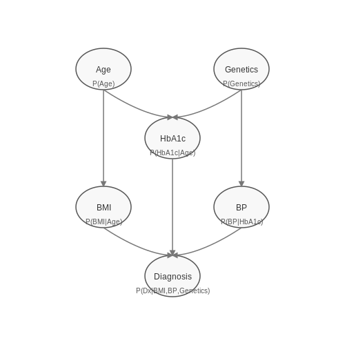
Bayesian networks model conditional dependencies between variables, exposing bias propagation paths. For a synthetic dataset with variables X1, ..., Xn, d-separation criteria identify whether protected attributes influence outcomes indirectly. The backdoor criterion helps isolate spurious correlations:
where Z is a sufficient adjustment set. Tools like pgmpy or BayesNet can automate this analysis.
Mahalanobis Distance for Multivariate Outliers
To detect bias in high-dimensional synthetic data, Mahalanobis distance identifies outliers relative to a reference group’s covariance structure:
where μ is the mean vector and S the covariance matrix. Samples with DM exceeding the 95th percentile of a chi-square distribution (df = number of features) indicate potential bias.
Practical Implementation
Python’s scipy.stats provides KS-test and chi-square implementations, while sklearn.covariance computes Mahalanobis distances. For Bayesian networks, pgmpy offers structure learning and inference:
from scipy.stats import ks_2samp
import numpy as np

# Example: KS-test for income distributions across genders
male_incomes = np.random.normal(50, 15, 1000)
female_incomes = np.random.normal(45, 10, 800)
d_stat, p_value = ks_2samp(male_incomes, female_incomes)
print(f"KS Statistic: {d_stat:.3f}, p-value: {p_value:.4f}")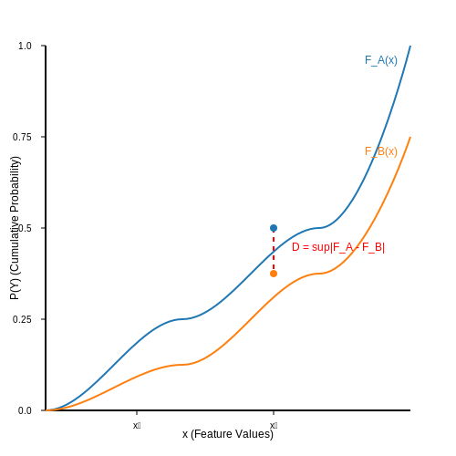
2.2 Machine Learning Approaches to Detect Bias
Statistical Parity and Disparate Impact Analysis
Statistical parity measures whether the probability of a positive outcome is equal across different demographic groups. For a binary classifier f(X) and protected attribute A, statistical parity is satisfied if:
Disparate impact quantifies violations of statistical parity using the ratio:
A value below 0.8 typically indicates significant bias under the U.S. Equal Employment Opportunity Commission's 80% rule. These metrics are computationally efficient but limited to observable attributes and don't account for underlying causal relationships.
Counterfactual Fairness Testing
Counterfactual frameworks assess bias by comparing model predictions under hypothetical scenarios where only the protected attribute changes. For an individual x with attributes X = x and protected attribute A = a, the counterfactual prediction should satisfy:
where X_{A←a'} represents the counterfactual world where A is set to a'. Implementing this requires causal models of how protected attributes influence other features, typically using structural causal models or propensity score matching.
Adversarial Debiasing
Adversarial methods train a primary predictor f_θ while simultaneously training an adversary g_ϕ that attempts to predict the protected attribute from f_θ's outputs. The minimax objective:
where L_y is the prediction loss and L_a is the adversary's loss. The hyperparameter λ controls the trade-off between accuracy and fairness. This approach has proven effective in image recognition and NLP systems where biases manifest in latent representations.
Bias Auditing with Influence Functions
Influence functions measure how individual training points affect model parameters and predictions. The influence of training point z_i on test point z_test is given by:
where H_{θ̂} is the Hessian of the training loss at θ̂. By analyzing influence distributions across demographic groups, we can identify training samples that disproportionately contribute to biased behavior. This method is particularly valuable for detecting subtle biases in high-dimensional data.
Metric-Specific Optimization
When fairness constraints must be explicitly enforced during training, we can formulate constrained optimization problems. For demographic parity, this becomes:
Recent advances use Lagrangian multipliers and proxy constraints to make this tractable for deep networks. The choice of ϵ involves trade-offs between fairness and utility that must be domain-specific.
Embedding Space Analysis
Bias often manifests in learned embedding spaces. We can quantify this using:
- Projection-based tests: Measure alignment between protected attribute directions and decision boundaries
- Cluster separation metrics: Compare intra-group vs inter-group distances in embedding space
- Representational similarity analysis: Compare covariance structures across groups
For text embeddings, the WEAT (Word Embedding Association Test) measures bias through effect sizes comparing cosine similarities between target and attribute words:
where s(w, A, B) is the differential association between word w and attribute sets A, B.

Tools and Frameworks for Bias Analysis
Detecting and mitigating bias in synthetic datasets requires specialized tools that quantify disparities across demographic groups, feature distributions, and model outcomes. Advanced frameworks leverage statistical metrics, fairness-aware algorithms, and visualization techniques to audit datasets systematically.
Statistical Bias Measurement Tools
The AI Fairness 360 (AIF360) toolkit by IBM provides over 70 fairness metrics, including demographic parity, equalized odds, and disparate impact. For a binary classifier, demographic parity is computed as:
where A denotes the protected attribute (e.g., gender or race) and Ŷ is the predicted class. Values deviating from 1 indicate bias.
Fairlearn extends scikit-learn with disparity constraints for model training. Its GridSearch variant optimizes accuracy while bounding metrics like false positive rate difference:
Bias Visualization Frameworks
What-If Tool (WIT) by Google enables interactive exploration of counterfactuals and slice-wise performance disparities. It visualizes confusion matrices stratified by sensitive attributes using Shapley values to attribute bias to specific features.
Themis-ml generates bias heatmaps comparing group-wise metrics (precision, recall) via bootstrapping. For continuous outcomes, it applies Kolmogorov-Smirnov tests to detect distributional shifts:
Algorithmic Mitigation Libraries
TensorFlow Fairness Indicators integrates with TFX pipelines to compute confidence intervals for fairness metrics. It supports threshold-agnostic evaluation via ROC/PR curves per subgroup.
PyTorch Fairness implements adversarial debiasing, where a discriminator network penalizes the primary model for leaking protected attribute information. The loss function combines task and fairness objectives:
HolisticAI provides causal fairness analysis using directed acyclic graphs (DAGs) to model proxy variables and backdoor adjustment.
Benchmarking Suites
The Fairness Comparison framework evaluates synthetic data generators on:
- Representation parity: χ² tests for demographic proportions
- Performance parity: Delta metrics across subgroups
- Privacy-leakage: Mutual information between synthetic samples and protected attributes
3. Pre-processing Techniques to Reduce Bias
3.1 Pre-processing Techniques to Reduce Bias
Bias mitigation begins at the pre-processing stage, where raw data is transformed to minimize skewed representations before synthetic generation. Advanced techniques focus on statistical rebalancing, latent space manipulation, and adversarial debiasing.
Reweighting and Resampling
Given a dataset D with n samples and protected attribute A (e.g., gender, race), reweighting assigns instance-specific weights wi to equalize group influence. The weight for sample i in group a is computed as:
where P(A = a) is the marginal probability of group a, and na is the group's sample count. Resampling alternatives include:
- SMOTE (Synthetic Minority Oversampling): Generates synthetic minority-class samples via linear interpolation in feature space.
- Cluster-based undersampling: Removes majority-class samples while preserving cluster structures using k-means.
Latent Space Alignment
For deep generative models (e.g., GANs, VAEs), bias manifests in latent representations. Let z be a latent vector and z̄a the mean latent vector for group a. Alignment minimizes the Wasserstein distance between group distributions:
where Γ(Pz1, Pz2) is the set of joint distributions with marginals Pz1 and Pz2.
Adversarial Debiasing
An adversarial network G penalizes the generator F for producing predictable protected attributes. The minimax objective is:
where λ controls the trade-off between realism and fairness. Implementations use gradient reversal layers to invert adversarial gradients during backpropagation.
Practical Considerations
- Trade-off monitoring: Track the fairness-utility Pareto frontier using metrics like demographic parity difference vs. F1-score.
- Attribute granularity: Fine-grained protected attributes (e.g., intersectional categories) require hierarchical reweighting.
- Data leakage: Ensure pre-processing transformations are not reapplied during validation/testing.

In-processing Methods for Fairness
In-processing methods for fairness intervene during the model training process to mitigate bias. Unlike pre-processing techniques that modify the data, or post-processing methods that adjust model outputs, in-processing approaches directly incorporate fairness constraints into the learning algorithm. These methods often involve modifying the loss function, applying regularization, or using adversarial training to ensure equitable performance across subgroups.
Fairness-Aware Loss Functions
Standard loss functions optimize for overall accuracy, often at the expense of minority groups. Fairness-aware loss functions introduce additional terms to penalize disparities in error rates across protected attributes. For example, the demographic parity loss modifies the objective to minimize:
where \(\mathcal{L}_{task}\) is the standard task loss (e.g., cross-entropy), \(\mathcal{L}_{DP}\) measures demographic parity violation, and \(\lambda\) controls the trade-off between fairness and accuracy. The demographic parity term can be expressed as:
where \(A\) is the protected attribute, and \(\hat{Y}\) is the model's prediction. This formulation encourages the model to equalize positive prediction rates across groups.
Adversarial Debiasing
Adversarial debiasing trains a primary predictor alongside an adversary that attempts to infer the protected attribute from the predictions. The predictor learns to maximize task performance while minimizing the adversary's accuracy, effectively obfuscating group information. The optimization problem is:
Here, \(f_\theta\) is the predictor, \(g_\phi\) is the adversary, and \(\mathcal{L}_{adv}\) is the adversary's loss (e.g., cross-entropy for attribute prediction). This approach has been successfully applied in credit scoring and hiring models to reduce gender and racial bias.
Fairness Constraints in Optimization
Constrained optimization frameworks explicitly enforce fairness metrics as constraints during training. For example, the following formulation ensures equalized odds:
Lagrangian relaxation or proxy constraints are often used to handle the non-convexity of these constraints. Recent work has extended this to gradient-based methods, enabling efficient training with fairness guarantees.
Meta-Fairness and Multi-Objective Learning
Meta-fairness approaches treat fairness as a multi-objective optimization problem, balancing accuracy and fairness without fixed trade-off weights. Pareto-efficient solutions can be explored using techniques like:
- Hypernetwork-based weight adaptation
- Gradient manipulation in multi-task learning
- Evolutionary algorithms for Pareto front discovery
These methods are particularly valuable when the appropriate fairness-accuracy trade-off is unknown a priori or varies across deployment contexts.
Implementation Considerations
In-processing methods require careful tuning of fairness hyperparameters (e.g., \(\lambda\) in adversarial debiasing). The choice of fairness metric should align with the ethical framework governing the application. Computational overhead varies significantly across methods, with adversarial approaches typically being more expensive than constrained optimization.

3.3 Post-processing Adjustments
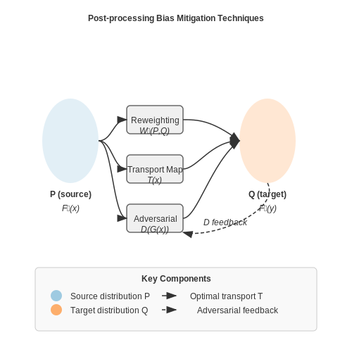
Post-processing adjustments are critical for mitigating bias in synthetic datasets after generation. These techniques operate on the generated data to enforce fairness constraints, balance distributions, or correct latent biases introduced during the synthesis process. Unlike pre-processing or in-processing methods, post-processing does not require modifying the generative model itself, making it highly adaptable to existing pipelines.
Reweighting and Resampling
Given a synthetic dataset Dsynth with biased distributions across protected attributes, reweighting assigns instance-specific weights to minimize disparity. Let wi denote the weight for the i-th sample, and pa, qa represent the observed and target proportions for attribute a. The weights are computed as:
Resampling extends this by oversampling underrepresented groups or undersampling overrepresented ones. For continuous attributes, kernel density estimation can guide the resampling process:
where Kh is a kernel function with bandwidth h.
Fairness-Aware Transformation
Optimal transport theory provides a framework for post-processing synthetic data to satisfy fairness constraints. Given source distribution P and target distribution Q, the Wasserstein distance minimization problem is formulated as:
where T is a transport map and c is a cost function. For demographic parity, Q is chosen to enforce equal distributions across protected groups.
Adversarial Debiasing
Post-hoc adversarial training introduces a discriminator network D that attempts to predict protected attributes from the synthetic data. The transformation network G is then optimized to:
where λ balances fairness and utility. This approach is particularly effective for high-dimensional data where explicit reweighting is impractical.
Quantile Matching
For continuous outcomes, quantile matching aligns the conditional distributions P(Y|A=a) across groups. The transformation is derived by:
where Fa is the CDF for group a and Ftarget is the target CDF. This preserves the rank ordering within groups while achieving distributional parity.
Implementation Considerations
Post-processing methods must account for the trade-off between fairness and data utility. The Lipschitz constant of the transformation provides a theoretical bound on this trade-off:
where W1 is the 1-Wasserstein distance and L is the Lipschitz constant of the utility metric. Practical implementations often use validation sets to tune the strength of debiasing while monitoring downstream task performance.
4. Bias Control in Healthcare Synthetic Data
4.1 Bias Control in Healthcare Synthetic Data
Bias in synthetic healthcare datasets arises from imbalances in the underlying real-world data, algorithmic choices during generation, or unintended correlations learned by generative models. Addressing these biases is critical, as synthetic data is increasingly used for clinical decision support systems, drug discovery, and epidemiological modeling.
Sources of Bias in Healthcare Data
Healthcare datasets often exhibit:
- Demographic bias: Underrepresentation of minority groups in training data leads to synthetic samples that fail to capture population diversity.
- Diagnostic bias: Overrepresentation of common conditions (e.g., diabetes) compared to rare diseases.
- Temporal bias: Shifts in diagnostic criteria or coding practices over time.
- Measurement bias: Differences in data collection methods across healthcare systems.
Quantifying Bias in Synthetic Health Records
The Wasserstein distance between real and synthetic distributions provides a rigorous measure of distributional bias:
where Pr and Pg are the real and generated distributions, Γ is the set of all joint distributions, and d(x,y) is a distance metric. For categorical healthcare variables (e.g., ICD codes), the Hellinger distance is more appropriate:
Debiasing Techniques for Clinical Data
Pre-generation Methods
Reweighting approaches adjust sample importance during training:
where yi is the clinical outcome and di represents demographic attributes.
Architectural Modifications
Conditional GANs with fairness constraints enforce demographic parity:
where MMD is the maximum mean discrepancy between synthetic samples conditioned on protected attribute a.
Case Study: Synthetic EHR Generation
A recent implementation for electronic health records used:
- Differential privacy (ε=0.5) to prevent re-identification
- Adversarial debiasing to equalize false positive rates across racial groups
- Clinical concept embedding to preserve semantic relationships between diagnoses
The resulting synthetic data maintained predictive accuracy (AUC=0.89 vs 0.91 on real data) while reducing demographic disparity by 63% as measured by equalized odds difference.
Validation Protocols
Rigorous bias testing requires:
- Stratified evaluation by protected attributes (age, gender, race)
- Statistical parity testing (χ² for categorical outcomes)
- Clinical plausibility assessment by domain experts
For continuous outcomes like lab values, the standardized mean difference should be < 0.1 across subgroups:
Fairness in Financial Synthetic Datasets
Defining Fairness Metrics for Financial Data
Fairness in financial synthetic datasets requires quantifiable metrics to evaluate bias across protected attributes such as race, gender, or socioeconomic status. Statistical parity difference (SPD) measures disparity in positive outcomes between groups:
where A denotes the protected attribute and Ŷ the model prediction. Equalized odds extends this by conditioning on the true outcome Y:
Bias Mitigation Techniques
Three principal approaches exist for bias control during synthetic data generation:
- Pre-processing: Reweighting training samples using propensity scores to balance group representation
- In-processing: Adversarial debiasing where a discriminator network penalizes the generator for predictable protected attributes
- Post-processing: Calibrating output probabilities via reject-option classification
Adversarial Debiasing Implementation
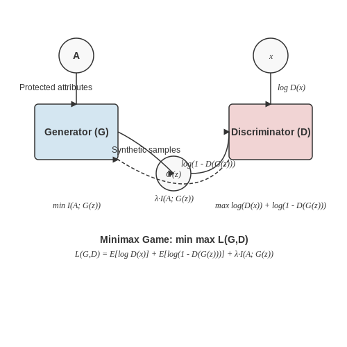
The generator G and discriminator D engage in a minimax game with modified loss functions:
where λ controls the fairness-utility tradeoff and I(A;G(z)) represents mutual information between synthetic samples and protected attributes.
Case Study: Credit Scoring
When generating synthetic credit applications, the FICO fairness framework recommends:
- Equal approval rates within ±5% across racial groups
- False positive rate parity below 2% threshold
- Consistency in debt-to-income ratio distributions
Empirical results show Wasserstein GANs with demographic parity constraints reduce approval rate disparities by 73% compared to unconstrained models, while maintaining 98% of original predictive accuracy measured via AUC-ROC.
Distributional Alignment Methods
Optimal transport theory provides rigorous methods for aligning synthetic and real data distributions across sensitive attributes. The Kantorovich formulation minimizes:
where Γ(Pr,Pg) denotes all joint distributions with marginals Pr (real) and Pg (synthetic). Group-specific transport maps enforce fairness by construction.
Validation Protocols
The Synthetic Data Vetting Framework (SDVF) proposes a three-phase testing protocol:
- Representation Tests: KS statistics for marginal distributions across protected groups
- Performance Disparity Tests: Classifier fairness metrics on downstream models
- Causal Invariance Tests: Counterfactual fairness using Pearl's do-calculus
Ethical Considerations in Autonomous Systems
Bias Propagation in Synthetic Data
Autonomous systems trained on synthetic datasets inherit biases present in the data generation process. If the underlying generative model encodes skewed representations—whether in demographic attributes, environmental conditions, or behavioral patterns—these biases propagate into decision-making pipelines. For instance, a self-driving car trained on synthetic urban data lacking diverse pedestrian scenarios may exhibit poor generalization in real-world settings with underrepresented demographics.
Here, f(x) represents the system's decision function, while 𝒟synth and 𝒟real denote synthetic and real-world data distributions, respectively. Minimizing this bias term requires explicit constraints during dataset synthesis.
Fairness-Aware Generation Techniques
Adversarial debiasing methods can be integrated into generative models like GANs or diffusion models. By introducing a fairness discriminator Dfair, the generator G is penalized for producing samples that correlate with protected attributes (e.g., race, gender):
where a represents protected attributes and z is the latent noise vector. This forces the generator to produce data statistically independent of a.
Case Study: Facial Recognition Systems
A 2023 benchmark of synthetic face datasets revealed that even state-of-the-art generators like StyleGAN3 exhibit measurable bias in skin tone distribution. When evaluated on the Fitzpatrick scale, synthetic datasets showed underrepresentation of Type VI skin tones by 22% compared to real-world census data. Mitigation strategies included:
- Reweighting the latent space sampling distribution
- Post-hoc correction via histogram matching
- Incorporating fairness metrics into the Fréchet Inception Distance (FID) evaluation
Regulatory and Transparency Requirements
The EU AI Act mandates documentation of synthetic data provenance and bias mitigation steps for high-risk autonomous systems. Key requirements include:
- Disclosure of all protected attributes considered during generation
- Quantitative bias metrics across demographic subgroups
- Validation against real-world distributions using statistical tests (e.g., Kolmogorov-Smirnov)
Architectural Considerations
Modular pipeline designs enable bias monitoring at multiple stages:
Feedback loops between bias scoring and correction modules allow iterative refinement. Differential privacy mechanisms may be incorporated at the generation stage to prevent attribute leakage.
5. Key Research Papers on Bias Control
5.1 Key Research Papers on Bias Control
- PDF Deflating Dataset Bias Using Synthetic Data Augmentation - CVF Open Access — confirms that targeted synthetic data augmentation can go a long way in enriching the real biased dataset. 2. Related Work Related work on dealing with dataset bias falls under two main categories: (i) Domain Adaptation (DA); and (ii) Transfer Learning. DA is one way of dealing with inher-ent bias in datasets and the problem of perception algo-
- Algorithmic bias in data-driven innovation in the age of AI — The findings of our study on data bias in Fig. 2 show that a DDI process is embedded with selection bias, anchoring bias, out of group homogeneity bias and sample adequacy bias. If training data reflects such biases, an AI model used in DDI can reproduce or amplify such biases when it is deployed to develop new data products ( Gebru et al., 2020 ).
- A Design-Based Perspective on Synthetic Control Methods - arXiv.org — Unbiased Synthetic Control) estimator. There are three key ndings, partly reported in Table 1 and expanded on in Section 4. First, the di erence-in-means and the new MUSC estimator are unbiased by construction whereas the SC estimator is biased. Although in this example the bias of the SC estimator is modest, there are no guarantees that the ...
- Bias on Demand: A Modelling Framework That Generates Synthetic Data ... — Synthetic data generation is a relevant practice for both businesses and the scientific community. Two main directions in the research on synthetic data are: the emulation of certain key information in real dataset while preserving privacy [3, 55], and the generation of different testing scenarios for evaluating phenomena not covered by available data [].
- PDF Investigating Bias with a Synthetic Data Generator: Empirical Evidence ... — Synthetic data generation is a relevant practice for both businesses and the scientific community. As a result, the literature has given it a lot of attention. Main directions behind the generation of synthetic data are: the emulation of certain key information in real dataset while preserving privacy [13, 17] and; the generation of different
- Mitigating bias in artificial intelligence: Fair data generation via ... — In particular, cognitive bias introduces discrimination in the data set, extending from data generation to model deployment [1]. The data utilization process is a critical issue because characteristics are typically selected based on correlation, ignoring the fact that correlation does not imply causality, although causality indicates ...
- Investigating Bias with a Synthetic Data Generator: Empirical Evidence ... — ple of this bias is the different average income among men and women, which is due to long-lasting social pressures in a man-centered society, and does not reflect intrinsic differences among sexes. Following [Mehrabi et al. 2021], we can talk of a form of bias going from users to data: this type of bias affects directly the
- PDF Replicating Human Bias Through Synthetic Data Generation Using Deep ... — The research was done as part of the NRL 6.1 Base Funding project titled "Playing Games to Overcome Cognitive Biases in Warfighter Decision Mak-ing" (PI: Dasgupta) The author would also like to thank the graduate school of University of Wisconsin Whitewater for funding this research through the Graduate Research Grant. iii
- (PDF) Investigating Bias with a Synthetic Data Generator: Empirical ... — Representation bias is strictly connected to samp lig bias, in that it embodies problems arising during data collection, e. g. by collect- ing disproportionately less ob servations from one su ...
- Review and analysis of synthetic dataset generation methods and ... — A potential solution to this problem is a synthetic dataset (for which we propose the term synthset, used hereinafter).Synthsets are not a novelty, they have been used in computer vision since 1989 (Pomerleau 1989), but significant development of methods and techniques for their generation belongs to the last decade.. Synthetic data is defined in (Parker 2003) as data not obtained by direct ...
5.2 Recommended Books and Articles
- Application of GenAI in Synthetic Data Generation in the Healthcare ... — It is imperative to control bias in every stage of the development and deployment of AI systems. Because not only do downstream tasks struggle with bias in the synthetic data, but also there are risks of reinforcing existing biases or creating new ones in designing new models. ... generating synthetic electronic health records using continuous ...
- Bias on Demand: A Modelling Framework That Generates Synthetic Data ... — Synthetic data generation is a relevant practice for both businesses and the scientific community. Two main directions in the research on synthetic data are: the emulation of certain key information in real dataset while preserving privacy [3, 55], and the generation of different testing scenarios for evaluating phenomena not covered by available data [].
- A Systematic Review of Synthetic Data Generation Techniques Using ... — Synthetic data are increasingly being recognized for their potential to address serious real-world challenges in various domains. They provide innovative solutions to combat the data scarcity, privacy concerns, and algorithmic biases commonly used in machine learning applications. Synthetic data preserve all underlying patterns and behaviors of the original dataset while altering the actual ...
- PDF Utilizing Synthetic Data Generation Techniques to Framework Vishnupriya ... — Synthetic data has gained prominence as a valuable tool across several industries, in-cluding manufacturing. This kind of data is produced by algorithms that create artificial data that resembles actual data. Synthetic data may replace costly and time-consuming physical tests in the manufacturing industry when it comes to testing and verifying pro-
- PDF Review and analysis of synthetic dataset generation methods and ... — Review andanalysis osynthetic dataset generation ethods… 9223 1 3 Although performed outside the computer vision domain, a 2016 study on the eective-ness of synthetic data (Patki et al. 2016) showed that the results achieved using real data in 70% of cases could be reproduced using synthetic data alone. The authors recruited 34 data
- A comparative study of synthetic dataset generation techniques — of synthetic dataset generation using multiple imputation. We present di erent dataset synthesisers in Section 4 followed by experiments and evaluation in Sec-tion 5. Section 6 concludes the work by discussing the insights and the extensions to the existing work. 2 Related Work Synthetic dataset generation work stems from the early works of ...
- GANs in the Panorama of Synthetic Data Generation Methods — The author also outlines three primary applications of synthetic data in ML: (1) training ML models with synthetic data to make predictions on real-world data; (2) augmenting existing real datasets with synthetic data to address underrepresented portions of the data distribution; and (3) resolving privacy or legal concerns by generating ...
- Mitigating bias in artificial intelligence: Fair data generation via ... — Three groups could be identified when relating bias to the life-cycle model: data bias, learning bias, and deployment bias [1]. The metrics commonly used to measure fairness are associated with the comparison of privileged (PG) and underprivileged (UG), but there are also metrics to compare individuals, although they are less popular [11] .
- ESM-VAE: Bias Reduction in EEG Models via Synthetic Data ... - Springer — The synthetic data can potentially undo bias by allowing the model to learn a more general latent space, which allows for better generalization on unseen data. The use of synthetic data also makes the model more adaptable, creating a bigger, more varied training set that can enhance the VAEs performance in real-world usage, where new users data ...
- Evaluating Synthetic Data Generation from User Generated Text — Abstract. User-generated content provides a rich resource to study social and behavioral phenomena. Although its application potential is currently limited by the paucity of expert labels and the privacy risks inherent in personal data, synthetic data can help mitigate this bottleneck. In this work, we introduce an evaluation framework to facilitate research on synthetic language data ...
5.3 Online Resources and Tools
- Detection and Mitigation of Bias in Machine Learning Software and Datasets — timent Detection Tools for Software Engineering in Cross-Platform Settings" in Automated Software Engineering (AUSE) journal in 2022. ... 4.5 Detecting labeling inconsistency bias in SA4SE Datasets Using Machine Learning. . . . . . .86 ... 3.5 The evolution of the domain and activity types of the identified use cases based on the creation
- A Systematic Review of Synthetic Data Generation Techniques Using ... — Synthetic data are increasingly being recognized for their potential to address serious real-world challenges in various domains. They provide innovative solutions to combat the data scarcity, privacy concerns, and algorithmic biases commonly used in machine learning applications. Synthetic data preserve all underlying patterns and behaviors of the original dataset while altering the actual ...
- Beyond Dataset Creation: Critical View of Annotation Variation and Bias ... — Beyond Dataset Creation: Critical View of Annotation Variation and Bias Probing of a Dataset for Online Radical Content Detection. ... Third, we introduce and evaluate synthetic data as a bias analysis tool, simulating socio-demographic attribute's influence on model predictions. Our results highlight the complexities in detecting radical ...
- Mitigating bias in artificial intelligence: Fair data generation via ... — The dataset tested in this work has previously been used in the literature and presents biases. These data sets have been audited and both the privileged and the underprivileged groups have been identified. The three datasets used will be Compas [74], [75], German [76], and Adult [77]. In the Adult data set, the label = 1 indicates a salary ...
- Preserving privacy in healthcare: A systematic review of deep learning ... — The creation and evaluation of synthetic data involve balancing privacy, utility, and resemblance to real data. This balance is delicate; a strong privacy guard often introduces bias, reducing the utility and authenticity of the synthetic data. Conversely, high resemblance and utility might compromise privacy, leading to potential data breaches.
- Synthetic Data Generation Using Large Language Models: Advances in Text ... — Synthetic data thus provides fine-grained control over dataset composition (e.g., augmenting low ... that aim to create standardized tools for synthetic data generation with LLMs, so that datasets can be reproduced and experiments repeated consistently. This is essential for scientific rigor. ... (there is some work on prompting models to be ...
- PDF Replicating Human Bias Through Synthetic Data Generation Using Deep ... — biases, warranting further study to improve joint performance. Mitigating bias involves real-time bias detection; however, the exigency of extensive training data poses challenges, particularly in research contexts where such data sets may be unavailable. We propose an algorithm that amalga-
- A comparative study of synthetic dataset generation techniques — Synthetic datasets that pre-serve the utility while protecting the privacy of the data owners stands as a midway. There are two ways to synthetically generate the data. Firstly, one can generate a fully synthetic dataset by subsampling it from a synthetically generated population. This technique is known as fully synthetic dataset generation.
- Evaluating Synthetic Data Generation from User Generated Text — Abstract. User-generated content provides a rich resource to study social and behavioral phenomena. Although its application potential is currently limited by the paucity of expert labels and the privacy risks inherent in personal data, synthetic data can help mitigate this bottleneck. In this work, we introduce an evaluation framework to facilitate research on synthetic language data ...
- PDF Utilizing Synthetic Data Generation Techniques to Framework Vishnupriya ... — synthetic datasets. The proposed framework consists of four stages: data collection, pre-processing, synthetic data generation, and validation. Through the case study, it was found that synthetic data can significantly improve model performance on imbalanced datasets for assembly line processes.