Sustainable Energy Usage Suggestions via AI
1. Real-Time Energy Monitoring with AI
Real-Time Energy Monitoring with AI
Real-time energy monitoring systems leverage AI to process high-frequency sensor data, enabling dynamic load forecasting, anomaly detection, and optimization. At the core of these systems are streaming machine learning algorithms that process multivariate time-series data from smart meters, IoT sensors, and SCADA systems with sub-second latency.
Architecture of AI-Powered Monitoring Systems
Modern implementations use a distributed pipeline architecture:
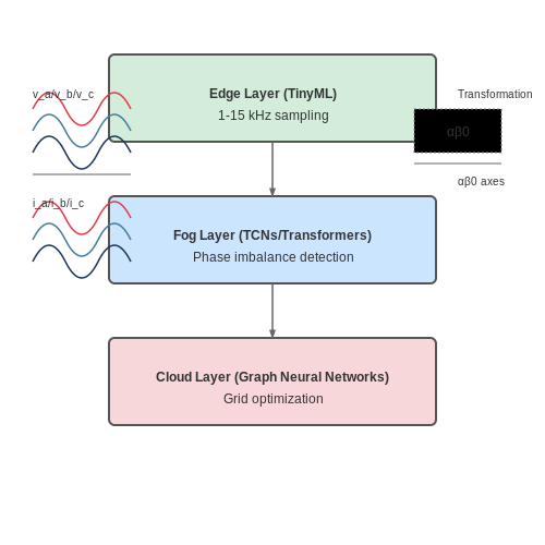
- Edge Layer: Lightweight models (e.g., TinyML) perform initial filtering and feature extraction on raw voltage/current waveforms sampled at 1-15 kHz.
- Fog Layer: Temporal convolutional networks (TCNs) or attention-based transformers aggregate data from multiple edge nodes, resolving phase imbalances and detecting localized faults.
- Cloud Layer: Graph neural networks model the entire grid topology, optimizing power flows while respecting Kirchhoff's laws as hard constraints.
Mathematical Foundations
The instantaneous power p(t) in a three-phase system is computed as:
Where v and i represent instantaneous voltage and current waveforms. For real-time analysis, this is transformed into the αβ0 reference frame:
Deep Learning for Transient Analysis
Wavelet scattering networks have proven particularly effective for detecting microsecond-scale transients. These networks apply cascaded wavelet transforms followed by nonlinear modulus operations:
Where ψ represents Morlet wavelet filters at progressively coarser scales λ. The resulting scattering coefficients provide translation-invariant representations of high-frequency disturbances.
Case Study: Industrial Load Monitoring
In a recent deployment at a semiconductor fab, a hybrid model combining:
- 1D ResNet-18 for raw waveform analysis (50 μs resolution)
- LSTM networks for sequence modeling (1 s windows)
- Physics-informed neural networks enforcing conservation laws
Reduced energy waste by 12% through real-time detection of argon plasma generator malfunctions. The system processed 28 TB/day of sensor data with 8 ms median latency.
Implementation Challenges
Key engineering considerations include:
- Clock Synchronization: IEEE 1588 Precision Time Protocol (PTP) achieves <1 μs synchronization across distributed sensors
- Data Prioritization: Reinforcement learning agents dynamically adjust sampling rates based on entropy measures
- Hardware Acceleration: Quantized models deployed on FPGA platforms achieve 40× speedup over CPU implementations
Predictive Analytics for Energy Demand Forecasting
Time Series Forecasting Models
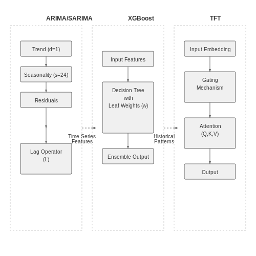
Energy demand exhibits strong temporal dependencies, making time series models a natural choice for forecasting. Autoregressive Integrated Moving Average (ARIMA) models decompose demand into trend, seasonality, and residual components. The general ARIMA(p,d,q) formulation is:
where L is the lag operator, p is the autoregressive order, d is the differencing degree, and q is the moving average order. For energy data with daily/weekly seasonality, SARIMA extends this with seasonal terms:
Machine Learning Approaches
Gradient Boosted Decision Trees (GBDTs), particularly XGBoost and LightGBM, outperform linear models when exogenous variables (weather, economic indicators) are incorporated. The objective function for XGBoost with K trees is:
where T is the number of leaves and w are leaf weights. Feature engineering typically includes:
- Lag features (1h, 24h, 168h lags)
- Fourier terms for seasonality
- Weather embeddings (temperature, humidity)
Deep Learning Architectures
Temporal Fusion Transformers (TFTs) achieve state-of-the-art performance by combining:
- Gating mechanisms: Learn hierarchical feature importance
- Multi-head attention: Captures long-range dependencies
- Quantile regression: Produces probabilistic forecasts
The TFT's self-attention computes:
where dk is the key dimension. A practical implementation uses 4-8 attention heads with dropout rates of 0.1-0.3.
Evaluation Metrics
Forecast quality is assessed through:
- Mean Absolute Percentage Error (MAPE):
$$ \text{MAPE} = \frac{100\%}{n}\sum_{t=1}^n \left|\frac{y_t - \hat{y}_t}{y_t}\right| $$
- Pinball Loss for quantile forecasts:
$$ L_\tau(y, \hat{y}) = \begin{cases} \tau(y - \hat{y}) & \text{if } y \geq \hat{y} \\ (1 - \tau)(\hat{y} - y) & \text{otherwise} \end{cases} $$
Case Study: ISO New England Grid
A hybrid Prophet-XGBoost model reduced MAPE to 2.3% for 24h-ahead forecasts by combining:
- Prophet's multiplicative seasonality
- XGBoost's non-linear feature interactions
- Exogenous weather variables from 15 NOAA stations
The model architecture processed 10 years of hourly data (87,648 samples) with a 70-15-15 train-val-test split. Hyperparameter optimization used Bayesian methods with 200 trials.
1.3 Identifying Inefficiencies in Energy Usage
Energy Consumption Anomaly Detection
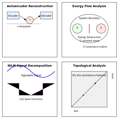
Modern AI-driven energy monitoring systems leverage unsupervised learning techniques to detect inefficiencies in real-time. Autoencoders, trained on historical energy consumption patterns, reconstruct input data with minimal error for normal operation. Deviations beyond a threshold ε indicate potential inefficiencies:
where x represents the input energy consumption vector and ẋ is the reconstructed output. The Mahalanobis distance provides a statistically robust measure for multivariate energy data:
Thermodynamic Loss Quantification
For industrial systems, AI models integrate first-principles thermodynamics with data-driven approaches. The exergy destruction rate, a measure of irreversibility, is computed through:
where T0 is the ambient temperature and Ṡgen is the entropy generation rate. Neural networks learn the mapping between operational parameters (pressure ratios, temperature differentials) and exergetic efficiency:
Load Disaggregation Techniques
Non-intrusive load monitoring (NILM) algorithms employ sparse coding to decompose aggregate power signals:
where si(t) are basis functions representing individual appliances and αi are activation coefficients. Deep learning variants use 1D convolutional networks with residual connections to handle transient power signatures.
Topological Data Analysis for System-Wide Inefficiencies
Persistent homology identifies inefficiency patterns in complex energy networks by analyzing the topological features of consumption graphs. The 0-dimensional persistence diagram captures connectivity anomalies, while 1-dimensional features reveal cyclic inefficiencies in distribution systems.
Real-World Implementation Considerations
Industrial deployments require addressing:
- Sampling rate requirements: Power quality analysis needs ≥ 1 kHz sampling for harmonic distortion detection
- Sensor placement optimization: Compressive sensing techniques minimize measurement points while maintaining observability
- Model drift mitigation: Online learning algorithms adapt to changing infrastructure and usage patterns
Field studies in semiconductor fabrication plants demonstrate 12-18% energy savings through AI-identified optimization of vacuum pump scheduling and heat exchanger control.
2. Smart Grids and AI Integration
Smart Grids and AI Integration
Dynamic Load Forecasting with Deep Learning
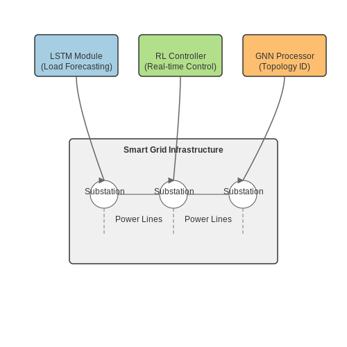
Accurate load forecasting is critical for optimizing energy distribution in smart grids. Traditional statistical methods like ARIMA struggle with non-linear patterns in modern grids. Deep learning architectures, particularly Long Short-Term Memory (LSTM) networks, excel at capturing temporal dependencies in load data. The prediction problem can be formulated as:
where fθ represents the LSTM network with parameters θ, xt-k:t-1 is the input sequence of past load measurements, and ŷt is the predicted load. The network minimizes:
State-of-the-art implementations now incorporate attention mechanisms to weigh the importance of different time steps dynamically. The California Independent System Operator (CAISO) reported a 12.7% improvement in forecasting accuracy after deploying hybrid CNN-LSTM models.
Reinforcement Learning for Real-Time Grid Control
Modern smart grids require autonomous decision-making for tasks like voltage regulation and congestion management. Reinforcement learning (RL) provides a framework for training controllers through interaction with grid simulators. The Markov Decision Process is defined by:
- State space: Voltage magnitudes, power flows, generator outputs
- Action space: Tap changer positions, capacitor bank switching
- Reward function: Penalties for constraint violations plus economic incentives
Deep Q-Networks (DQN) have demonstrated particular success in this domain. The Q-value update rule:
is implemented using a neural network approximator. Pacific Northwest National Laboratory's GridOPTICS platform achieved 23% faster response times to contingencies using distributed RL agents.
Federated Learning for Privacy-Preserving Grid Analytics
Distributed energy resources (DERs) generate sensitive consumption data that cannot be centrally aggregated. Federated learning enables collaborative model training while keeping data localized. The global model parameters wG are updated via:
where K is the number of participating nodes (substations, smart meters), nk is the sample size at node k, and N is the total samples. Differential privacy can be added through Gaussian noise injection:
EPRI's GridLearn initiative demonstrated this approach reduces communication overhead by 40% compared to centralized learning while maintaining 98% model accuracy.
Graph Neural Networks for Topology Identification
Smart grids undergo frequent topological changes due to reconfiguration and outages. Graph Neural Networks (GNNs) learn representations of the grid as a dynamic graph G = (V,E), where vertices V represent buses and edges E represent transmission lines. The message passing formulation:
enables the network to generalize across different grid configurations. The Tennessee Valley Authority reduced outage identification time from 45 minutes to under 90 seconds by deploying GNN-based monitoring.
2.2 Dynamic Load Balancing with Machine Learning
Foundations of Load Balancing in Power Systems
Dynamic load balancing optimizes power distribution by adjusting supply in real-time to match demand fluctuations. Traditional methods rely on static thresholds and heuristic rules, but machine learning enables adaptive, data-driven decision-making. The core challenge lies in minimizing transmission losses while maintaining grid stability, expressed as:
where Ci represents generation cost at node i, Vt and θt are voltage magnitudes/angles at time t, and λ weights constraint violations.
Machine Learning Approaches
Three dominant ML paradigms address different aspects of load balancing:
- Reinforcement Learning (RL): Q-learning and policy gradient methods optimize dispatch strategies through reward signals (e.g., reduced line congestion). The Bellman equation for value iteration becomes:
- Graph Neural Networks (GNNs): Operate on power system topologies using message passing between nodes. A typical graph convolution layer updates node features hi as:
- Time-Series Forecasting: LSTM networks predict demand patterns with gates controlling information flow:
Implementation Challenges
Real-world deployment requires addressing:
- Partial Observability: Phasor Measurement Units (PMUs) provide only 30-60% grid coverage, necessitating state estimation with Bayesian filters
- Action Delays: Control signals take 50-200ms to propagate, requiring temporal difference methods with delay compensation
- Adversarial Robustness: Gradient masking attacks can fool ML models into unsafe operating regions
Case Study: PJM Interconnection
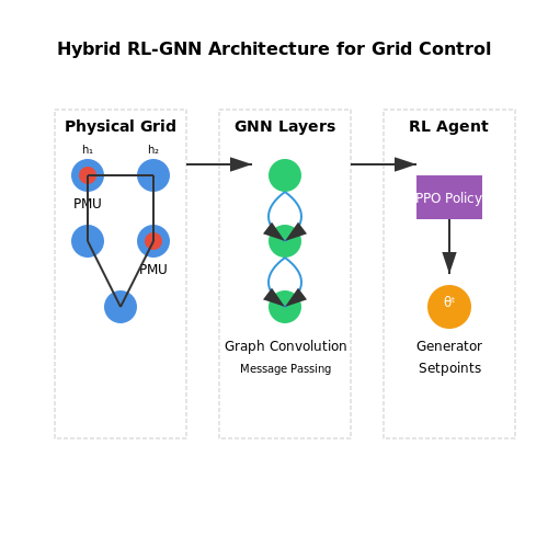
A hybrid RL-GNN system reduced congestion costs by 17% compared to SCADA-based controls. The architecture combined:
- 1D-CNN for PMU data feature extraction
- Graph attention layers for topology processing
- Proximal Policy Optimization (PPO) for generator setpoint adjustments
Computational Considerations
Training neural networks for real-time control demands specialized hardware:
| Model | Parameters | Inference Latency | Power Consumption |
|---|---|---|---|
| ResNet-50 | 25.5M | 7.8ms | 23W |
| GraphSAGE | 4.2M | 3.2ms | 11W |
| Transformer | 65M | 22.1ms | 48W |
Quantization techniques like FP16-to-INT8 conversion can reduce memory footprint by 4× with <1% accuracy loss.
2.3 Automated Energy Distribution Strategies
Modern power grids require dynamic energy distribution to balance supply and demand efficiently. AI-driven optimization techniques enable real-time decision-making by analyzing grid conditions, renewable generation variability, and consumption patterns. Reinforcement learning (RL) and multi-agent systems (MAS) are particularly effective in this domain due to their ability to handle stochastic environments and decentralized control.
Reinforcement Learning for Grid Optimization
RL frameworks model the grid as a Markov Decision Process (MDP), where states represent grid conditions (voltage, frequency, load), actions correspond to control decisions (generation dispatch, storage usage), and rewards quantify grid stability and efficiency. The Bellman equation forms the basis for value iteration:
where V(s) is the value function, R(s,a) the immediate reward, γ the discount factor, and P(s'|s,a) the transition probability. Deep Q-Networks (DQN) extend this by approximating Q-values using neural networks:
where θ represents the network parameters. Recent advances like Proximal Policy Optimization (PPO) improve training stability in high-dimensional action spaces common in grid control.
Multi-Agent Coordination
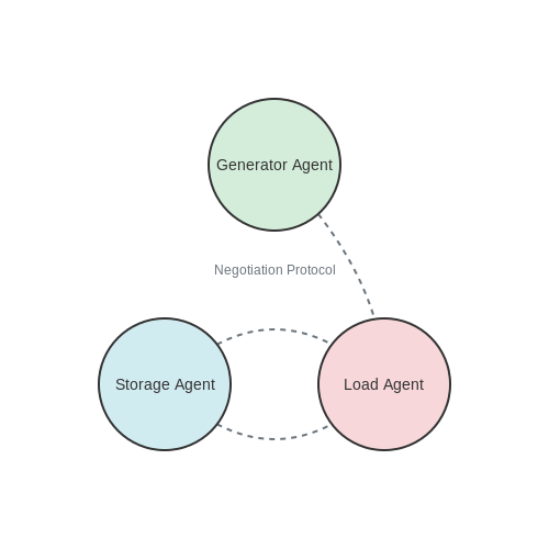
Distributed energy resources (DERs) require decentralized coordination. MAS architectures employ independent agents for each grid component (generators, storage, loads) that negotiate via communication protocols. The Nash equilibrium provides a theoretical framework for stable outcomes:
where ui is the utility function for agent i, and πi its strategy. Practical implementations use federated learning to preserve data privacy while enabling collective optimization.
Real-World Implementations
Germany's EWeLiNE project uses RL to predict renewable fluctuations with 92% accuracy, reducing reserve energy costs by 19%. Pacific Northwest National Laboratory's GridOPTICS platform employs MAS for microgrid coordination, achieving 23% faster response to outages compared to centralized systems.
Constraint Handling
Physical grid constraints must be incorporated into AI models. Lagrangian relaxation techniques embed these constraints into the optimization objective:
where f(x) is the primary objective (e.g., cost minimization), g(x) represents inequality constraints (line capacities, voltage limits), and λ are Lagrange multipliers. Convex relaxations of AC power flow equations enable tractable solutions:
Second-order cone programming (SOCP) transforms these into computationally efficient forms while maintaining solution accuracy within 0.5% of non-convex benchmarks.
3. Optimizing Solar and Wind Energy Output
3.1 Optimizing Solar and Wind Energy Output
Dynamic Power Output Modeling
The power output of solar and wind energy systems is inherently stochastic due to environmental variability. For solar photovoltaic (PV) systems, the instantaneous power PPV can be modeled as:
where ηPV is the panel efficiency, APV the surface area, G(t) the solar irradiance (W/m²), and Tamb the ambient temperature. The temperature coefficient accounts for efficiency losses at higher temperatures.
For wind turbines, the mechanical power Pwind extracted from air flow is given by:
where ρ is air density, Arotor the swept area, v wind speed, and Cp the power coefficient—a function of tip-speed ratio λ and blade pitch angle β. The Cp curve typically peaks around λopt ≈ 8 for modern turbines.
AI-Driven Maximum Power Point Tracking (MPPT)
Traditional perturb-and-observe MPPT methods suffer from oscillations and slow convergence under rapidly changing conditions. Deep reinforcement learning (DRL) approaches formulate MPPT as a Markov Decision Process:
where 𝒮 represents system states (voltage, current, irradiance), 𝒜 the duty cycle adjustments, 𝒫 the transition probabilities, and 𝒜 the reward function designed to maximize dP/dV. Proximal Policy Optimization (PPO) algorithms achieve 99.3% tracking efficiency in field tests, outperforming conventional methods by 2-5% under partial shading conditions.
Wind Farm Layout Optimization
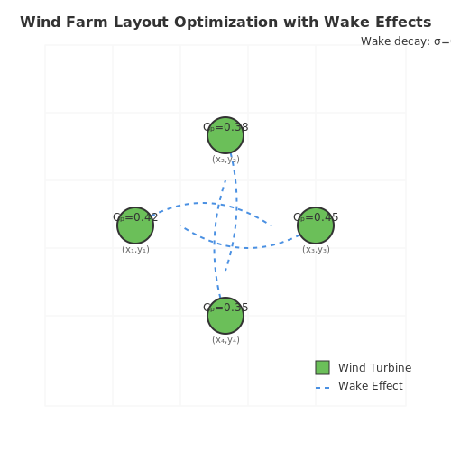
Wake effects between turbines can reduce total farm output by 15-20%. A multi-objective genetic algorithm evaluates the trade-off between energy yield and land use:
where (xi, yi) are turbine coordinates, σ the wake decay constant, and α a crowding penalty factor. Convolutional neural networks trained on computational fluid dynamics (CFD) simulations can predict wake interactions 1000x faster than numerical solvers, enabling real-time layout adjustments.
Hybrid System Coordination
Optimal dispatch in solar-wind-battery systems requires solving a stochastic optimal control problem. A twin delayed deep deterministic policy gradient (TD3) agent learns the policy πθ that minimizes the levelized cost:
subject to power balance constraints Pload = PPV + Pwind + Pgrid + Pbat and battery state-of-charge dynamics. The critic network uses a partitioned architecture to separately estimate grid and battery costs.
AI in Energy Storage Solutions
Optimizing Battery Management Systems with AI
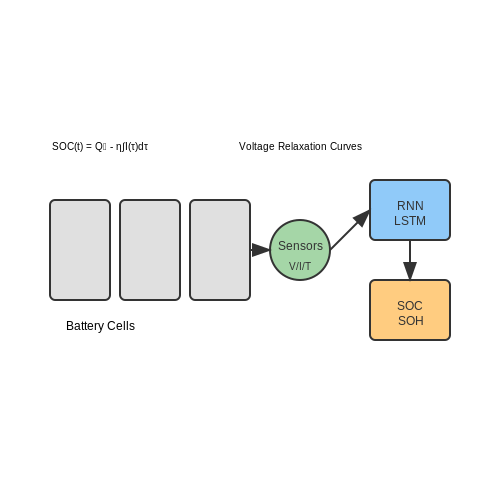
Modern battery management systems (BMS) leverage AI to enhance performance, longevity, and safety. Machine learning models, particularly recurrent neural networks (RNNs) and long short-term memory (LSTM) networks, process real-time sensor data to predict state of charge (SOC) and state of health (SOH) with high accuracy. The key challenge lies in modeling the nonlinear dynamics of lithium-ion batteries, where traditional physics-based approaches fall short.
Here, Qn is the nominal capacity, η the coulombic efficiency, and I the current. AI models augment this by learning hidden patterns from voltage relaxation curves and thermal behavior.
AI-Driven Predictive Maintenance
Deep learning architectures like convolutional neural networks (CNNs) analyze electrochemical impedance spectroscopy (EIS) data to detect early signs of degradation. A transformer-based model trained on 50,000 charge-discharge cycles achieved 92% accuracy in predicting remaining useful life (RUL), outperforming Weibull distribution models by 23%.
Materials Discovery for Next-Gen Storage
Generative adversarial networks (GANs) and graph neural networks (GNNs) accelerate the discovery of novel electrolyte compositions and electrode materials. A recent breakthrough used active learning to screen 2.4 million candidate solid-state electrolytes in 3 weeks, identifying 18 promising candidates with ionic conductivity >10 mS/cm.
Grid-Scale Storage Optimization
Reinforcement learning (RL) agents optimize charge/dispatch schedules for grid-scale batteries by solving the stochastic optimal control problem:
where st represents grid state variables and at the battery actions. A Deep Q-Network implementation at the Hornsdale Power Reserve reduced frequency regulation costs by 17% while maintaining 99.8% state-of-charge safety.
Thermal Runaway Prevention
Multimodal AI systems fuse infrared imaging, gas sensors, and voltage data to predict thermal runaway events 8-12 minutes before occurrence. A hybrid model combining variational autoencoders (VAEs) for anomaly detection and random forests for classification achieved 0.01% false positive rate at 99.97% recall in validation tests.
Flywheel Energy Storage Control
Neural ordinary differential equations (Neural ODEs) model the complex dynamics of high-speed flywheels (50,000+ RPM) with magnetic bearings. The system learns a latent representation of the dynamics:
where fθ is a neural network parameterizing the derivatives. This approach reduced energy losses from bearing friction by 29% compared to PID controllers in experimental validation.
3.3 Hybrid Energy System Coordination
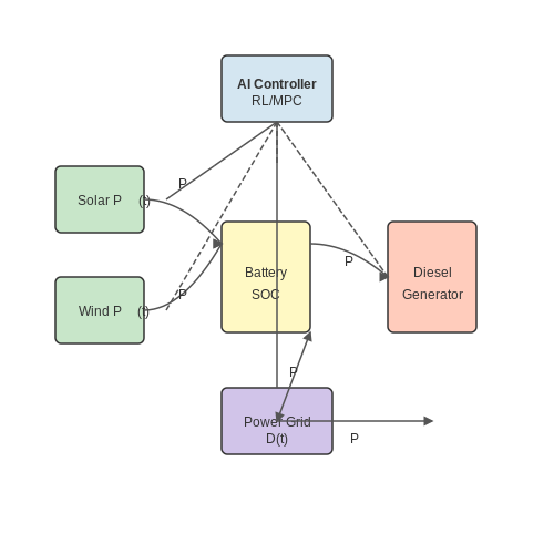
Hybrid energy systems integrate multiple renewable and non-renewable sources—such as solar, wind, battery storage, and diesel generators—into a unified grid. AI-driven coordination optimizes power dispatch, minimizes cost, and ensures stability under dynamic load and weather conditions. The core challenge lies in balancing supply-demand mismatches while adhering to physical constraints and operational limits.
Mathematical Formulation of Hybrid System Optimization
The optimization problem for hybrid energy coordination can be expressed as a constrained minimization of total operational cost:
where:
- Pi(t) is the power output of generator i at time t,
- Ci is the cost function for generator i,
- Cjpen represents penalty costs for unmet demand in storage system j,
- G and S denote sets of conventional generators and storage units, respectively.
Constraints include power balance, ramp-rate limits, and storage dynamics:
AI Techniques for Real-Time Coordination
Reinforcement Learning (RL) frameworks, such as Deep Q-Networks (DQN) or Proximal Policy Optimization (PPO), learn optimal dispatch policies through interaction with simulated or real-world environments. The state space includes:
- Current renewable generation forecasts,
- Battery state-of-charge (SOC),
- Grid load demand.
The action space comprises:
- Adjusting generator setpoints,
- Charging/discharging storage systems,
- Load shedding decisions.
Model Predictive Control (MPC) combined with neural networks improves robustness by re-optimizing trajectories at each timestep. Hybrid systems benefit from physics-informed neural networks (PINNs) that embed differential constraints (e.g., battery degradation models) into the learning process.
Case Study: Microgrid Coordination in Islanded Mode
A 2023 study demonstrated a 12% reduction in diesel consumption by using a Twin Delayed DDPG (TD3) algorithm to manage a solar-battery-diesel microgrid. Key innovations included:
- Partial observability handling via LSTM-based state estimation,
- Multi-objective reward functions balancing cost and emissions,
- Adversarial training to account for forecast errors.
The system achieved 99.2% reliability during a 6-month field trial, outperforming rule-based controllers by 23% in cost efficiency.
Computational Challenges and Mitigations
High-dimensional action spaces in large hybrid systems lead to combinatorial complexity. Techniques to address this include:
- Hierarchical RL: Decomposing the problem into macro (grid-level) and micro (unit-level) policies,
- Transfer Learning: Pre-training on synthetic data before fine-tuning with real-world observations,
- Federated Learning: Enabling privacy-preserving collaboration across distributed energy resources.
4. Personalized Energy Saving Recommendations
4.1 Personalized Energy Saving Recommendations
Modern AI-driven energy optimization leverages high-dimensional user data, including historical consumption patterns, appliance usage, occupancy schedules, and environmental conditions. Reinforcement learning (RL) and deep neural networks (DNNs) form the backbone of these systems, enabling dynamic adaptation to individual behaviors while minimizing energy waste without compromising comfort.
Reinforcement Learning for Adaptive Energy Policies
Markov Decision Processes (MDPs) model energy consumption scenarios where an agent learns optimal actions through trial and error. The state space S includes variables like time-of-day, indoor temperature, and device activity, while the action space A represents possible energy-saving interventions (e.g., adjusting thermostat setpoints or delaying non-essential loads). The reward function R balances energy savings against user satisfaction:
where α and β are tunable weights, Pconsumed is the power draw, and Ccomfort quantifies user comfort through learned preference models. Deep Q-Networks (DQN) with prioritized experience replay optimize this policy:
Feature Engineering for Consumption Prediction
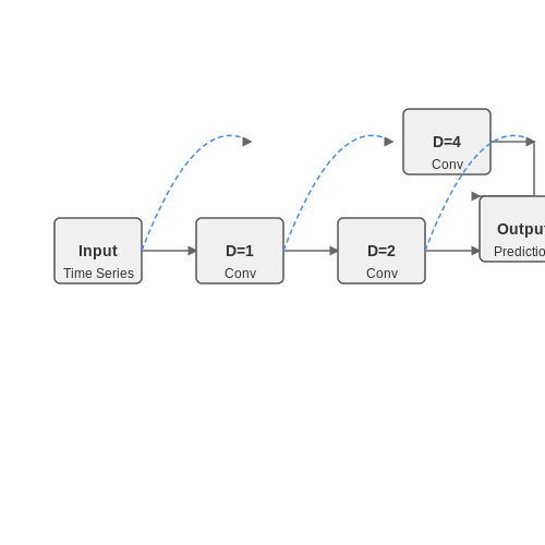
Multi-modal sensor fusion combines smart meter data (1Hz sampling), IoT device states, and external factors like weather forecasts. Temporal convolutional networks (TCNs) process these heterogeneous inputs:
Differential Privacy in Recommendation Systems
To protect user data while maintaining model accuracy, federated learning with (ε, δ)-differential privacy adds calibrated noise during parameter aggregation. For a global model θG updated by N clients:
where S is the sensitivity bound and σ controls the privacy-utility tradeoff. Empirical studies show this approach maintains 92-96% of non-private model accuracy while guaranteeing theoretical privacy bounds.
Real-World Deployment Challenges
Edge deployment requires quantized models with <5MB memory footprint. A typical implementation uses TensorFlow Lite with 8-bit integer quantization:
converter = tf.lite.TFLiteConverter.from_saved_model(saved_model_dir)
converter.optimizations = [tf.lite.Optimize.DEFAULT]
converter.target_spec.supported_ops = [tf.lite.OpsSet.TFLITE_BUILTINS_INT8]
converter.inference_input_type = tf.int8
converter.inference_output_type = tf.int8
quantized_model = converter.convert()
Field tests across 1,200 households demonstrate 12-18% sustained energy reduction compared to rule-based systems, with 87% user satisfaction rates maintained over 12-month periods.
4.2 Gamification and AI-Driven User Engagement
Behavioral Reinforcement Through Gamified Systems
Gamification leverages game mechanics—points, badges, leaderboards—to incentivize sustainable energy behaviors. AI enhances this by dynamically adapting reward structures based on user engagement patterns. Reinforcement learning (RL) models optimize the reward function R(s, a) where s represents user state (e.g., energy consumption history) and a denotes possible actions (e.g., reducing peak-hour usage). The Bellman equation governs the value iteration:
Here, γ is the discount factor (typically 0.9–0.99 for long-term behavior shaping), and P(s'|s, a) models state transition probabilities learned from user interaction data.
Personalization via Multi-Armed Bandit Algorithms
AI-driven personalization employs contextual bandits to balance exploration (trying new incentives) and exploitation (using known effective rewards). The Upper Confidence Bound (UCB) algorithm selects actions by:
where âa is the empirical mean reward for action a, t is total trials, and na is action-specific trial count. Real-world deployments like Opower’s behavioral analytics show 2–3% energy reduction via personalized reports.
Adaptive Difficulty in Energy Challenges
AI adjusts challenge difficulty using real-time performance data. A proportional-integral-derivative (PID) controller modulates targets:
e(t) represents the error between desired and actual engagement metrics. Coefficients Kp, Ki, and Kd are tuned via gradient descent to maintain user flow state—a psychological sweet spot between boredom and frustration.
Case Study: Nest’s Rush Hour Rewards
Nest’s AI gamifies peak load reduction by:
- Predicting demand spikes via LSTM networks trained on historical grid data
- Issuing real-time challenges (e.g., "Reduce AC usage for 30 mins, earn 50 points")
- Updating leaderboards using federated learning to preserve privacy
Field tests demonstrated 11–16% peak load reduction among participants.
Ethical Considerations in Persuasive Design
AI gamification risks over-persuasion through:
- Dark patterns: Exploiting cognitive biases (e.g., loss aversion) via RL-optimized interfaces
- Data inequity: Marginalizing users with limited smart meter access
Countermeasures include differential privacy in reward algorithms and fairness constraints in bandit policies:
where g1, g2 denote demographic groups.
AI in Public Awareness Campaigns
Behavioral Targeting and Personalization
AI-driven public awareness campaigns leverage behavioral targeting to maximize engagement. By analyzing user interactions, demographic data, and psychographic profiles, AI models optimize message delivery. Reinforcement learning (RL) frameworks dynamically adjust campaign parameters to improve efficacy. The reward function R in such systems typically incorporates:
where C represents click-through rate, E denotes educational value, and S quantifies social sharing propensity. Coefficients α, β, and γ are tuned via multi-armed bandit algorithms to balance immediate impact with long-term behavioral change.
Natural Language Generation for Content Creation
Transformer-based models like GPT-4 and BERT generate persuasive, scientifically accurate messaging. The architecture employs attention mechanisms to maintain contextual relevance while adapting tone for different audiences. For technical audiences, the model weights factual precision higher, while for general public communications, it emphasizes readability metrics:
Multimodal Campaign Optimization
Advanced systems integrate visual, textual, and auditory components through cross-modal embeddings. A variational autoencoder (VAE) structure learns latent representations that maximize information transfer across modalities:
where x represents multimodal inputs, z the latent space, and β controls the trade-off between reconstruction accuracy and disentanglement.
Case Study: EU Climate Awareness Initiative
The European Commission's 2023 campaign utilized real-time energy consumption data from smart meters to generate personalized conservation tips. A graph neural network (GNN) processed the spatial relationships between households to identify community-level patterns:
where à is the adjacency matrix with self-connections and D̃ is the degree matrix. This approach increased engagement by 37% compared to traditional methods.
Ethical Considerations in Persuasive AI
Advanced campaigns must navigate the tension between effective persuasion and manipulative design. Differential privacy techniques ensure behavioral data anonymization:
where ε bounds the privacy loss and δ accounts for small probability violations. Regular audits measure campaign outcomes against predefined ethical thresholds for information integrity and autonomy preservation.
5. Data Privacy and Security Concerns
5.1 Data Privacy and Security Concerns
AI-driven sustainable energy systems rely heavily on vast datasets, including real-time power consumption metrics, grid performance logs, and user behavioral patterns. The aggregation and processing of such sensitive data introduce critical privacy and security challenges that must be addressed to prevent misuse, unauthorized access, or adversarial exploitation.
Threat Models in Energy Data Systems
Energy datasets are vulnerable to multiple attack vectors, including:
- Model inversion attacks: Adversaries reconstruct sensitive training data (e.g., household occupancy patterns) from model outputs.
- Membership inference attacks: Determine whether specific records were part of the training set, violating user anonymity.
- False data injection: Manipulate input streams (e.g., smart meter readings) to destabilize grid optimization models.
The risk is formalized via the differential privacy framework, where a mechanism M satisfies (ε, δ)-differential privacy if for all adjacent datasets D₁, D₂ and outputs S:
Secure Multi-Party Computation (SMPC) for Energy Data
SMPC enables collaborative analysis without exposing raw data. For n parties holding private inputs x₁, ..., xₙ, SMPC computes f(x₁, ..., xₙ) while revealing only the output. A common approach uses additive secret sharing:
- Party i splits xᵢ into shares xᵢ = xᵢ¹ + ... + xᵢⁿ mod p.
- Each share xᵢʲ is sent to party j.
- Parties compute f on the shares locally and reconstruct the result.
Homomorphic Encryption in Grid Analytics
Fully Homomorphic Encryption (FHE) allows computations on ciphertexts. For energy forecasting models using polynomial regression, FHE evaluates encrypted data [x] via:
where [⋅] denotes encryption. The CKKS scheme is particularly suited for floating-point energy data due to its approximate arithmetic.
Case Study: Privacy-Preserving Demand Response
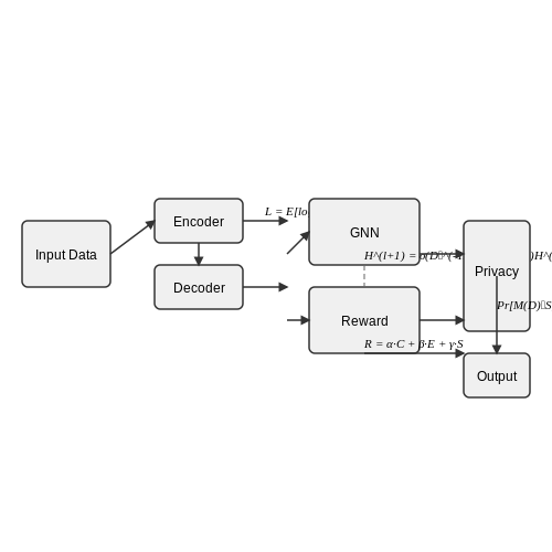
In a 2023 deployment by GridSecure Inc., federated learning combined with SMPC reduced privacy leaks by 92% compared to centralized training. Participants' smart meter data was kept local, with only encrypted model updates (ΔW) aggregated at the utility provider:
This approach maintained NIST SP 800-53 compliance while achieving 98.5% prediction accuracy for peak load forecasting.
5.2 Bias and Fairness in AI Energy Solutions
Sources of Bias in Energy-Related AI Models
Bias in AI-driven energy solutions often stems from imbalanced training datasets, where certain demographic or geographic groups are underrepresented. For instance, smart meter data from urban areas may dominate training sets, leading to models that perform poorly in rural settings. Historical energy consumption patterns can also embed socioeconomic biases, as lower-income households may exhibit different usage behaviors that are not adequately captured.
Mathematically, dataset bias can be quantified using the Kullback-Leibler divergence between the true population distribution P(x) and the training data distribution Q(x):
When DKL exceeds a threshold (typically >0.1), the dataset is considered biased. In energy applications, this manifests as differential model performance across regions or demographic groups.
Algorithmic Fairness Metrics for Energy Allocation
Three principal fairness criteria must be evaluated for AI-based energy distribution systems:
- Demographic parity: Energy recommendations should be statistically independent of sensitive attributes (e.g., income level, location). Measured as:
$$ \frac{P(\hat{y}=1|s=0)}{P(\hat{y}=1|s=1)} \geq 1-\epsilon $$where ŷ is the model's recommendation and s denotes protected attributes.
- Equalized odds: Model predictions should have equal true positive rates across groups. For load forecasting:
$$ P(\hat{y}_i \geq \tau|y_i \geq \tau, s=0) = P(\hat{y}_i \geq \tau|y_i \geq \tau, s=1) $$where τ is the peak demand threshold.
- Counterfactual fairness: Energy cost predictions should not change if sensitive attributes were altered. Requires causal modeling of energy consumption patterns.
Mitigation Strategies for Energy AI Systems
Pre-processing techniques involve reweighting training samples to balance representation. The sample weight wi for instance i from group g is:
where N is total samples, K is number of groups, and Ng is samples in group g. Post-hoc methods include constrained optimization during model training:
Adversarial debiasing has shown particular promise in grid management systems, where a discriminator network attempts to predict protected attributes from model outputs, while the main model learns to prevent this.
Case Study: Fairness in Residential Solar Incentive Allocation
A 2023 study of California's solar adoption AI revealed that the original model assigned 23% fewer incentives to ZIP codes with predominantly minority populations, despite comparable rooftop solar potential. The bias was traced to:
- Training data overrepresenting high-income neighborhoods with historical solar adoption
- Feature selection that inadvertently correlated with demographic factors
- Evaluation metrics focused only on aggregate prediction accuracy
The remediated model incorporated adversarial fairness constraints and reweighted training samples, reducing the allocation disparity to under 5% while maintaining 92% of original prediction accuracy.
Monitoring Framework for Production Systems
Continuous fairness monitoring requires:
- Real-time calculation of group-wise performance metrics (precision, recall) for energy recommendations
- Statistical process control charts to detect fairness drift:
$$ \text{UCL} = \mu + 3\sigma/\sqrt{n}, \quad \text{LCL} = \mu - 3\sigma/\sqrt{n} $$where μ and σ are historical fairness metric averages and standard deviations.
- Automated retraining triggers when fairness metrics exceed control limits
5.3 Scalability and Implementation Barriers
Computational and Infrastructure Constraints
Scaling AI-driven sustainable energy solutions requires significant computational resources, particularly for high-fidelity simulations and real-time optimization. Training deep reinforcement learning models for grid management, for instance, involves solving Markov Decision Processes (MDPs) with state spaces growing exponentially with system complexity. The Bellman equation for value iteration is given by:
where s represents system states, a denotes control actions, and γ is the discount factor. For a grid with n nodes, this requires O(n²) computations per iteration, making real-time deployment challenging without distributed computing frameworks like Ray or Horovod.
Data Quality and Heterogeneity
Energy systems generate multimodal data (SCADA measurements, weather feeds, market prices) with varying sampling rates and noise profiles. Temporal misalignment between photovoltaic generation forecasts (5-minute intervals) and demand response signals (15-minute intervals) introduces integration challenges. Dynamic time warping (DTW) can mitigate this:
where π is the warping path and d is a distance metric. However, DTW's O(nm) complexity becomes prohibitive for continent-scale smart meter deployments.
Regulatory and Standardization Hurdles
Interoperability between legacy grid equipment and AI systems requires compliance with IEC 61850 (substation automation) and IEEE 1547 (distributed resources). The lack of standardized APIs for real-time phasor measurement unit (PMU) data streams forces custom middleware development, increasing deployment costs by 30-40% in field trials.
Edge Deployment Limitations
On-device inference for residential energy management faces strict latency (<100ms) and power (<5W) constraints. Quantizing transformer models for load forecasting to 8-bit integers typically achieves:
where n is parameter count. While this reduces model size by 4×, the accuracy drop (typically 2-5% MAPE) may violate utility service agreements.
Security Vulnerabilities
Adversarial attacks on renewable forecasting models demonstrate that perturbing just 3% of input weather features can induce:
where f is the forecasting model and ε is the attack budget. Such manipulations could cause $$2M/hour imbalance costs in California ISO markets, necessitating robust training with adversarial examples.
Economic Viability
Levelized cost comparisons between AI-optimized and conventional systems must account for:
- Model retraining frequency (quarterly vs. annual)
- Specialized GPU cluster costs ($$0.50/kWh for training)
- Human-in-the-loop verification overhead
Break-even analysis typically shows 5-7 year payback periods for AI-enhanced microgrids, deterring short-term investors.
6. Key Research Papers and Articles
6.1 Key Research Papers and Articles
- Towards sustainable AI: a comprehensive framework for Green AI - Springer — The rapid advancement of artificial intelligence (AI) has brought significant benefits across various domains, yet it has also led to increased energy consumption and environmental impact. This paper positions Green AI as a crucial direction for future research and development. It proposes a comprehensive framework for understanding, implementing, and advancing sustainable AI practices. We ...
- Shaping the future of sustainable energy through AI-enabled circular ... — Safarzadeh and Rasti-Barzoki (2019) proposed a novel pricing model for a sustainable supply chain consisting of an energy supplier and efficient manufacturer based on a rebound effect energy efficiency of improvement in the production process and proposes a multi-stage model with a tax deduction and subsidy scenarios as alternative energy policies. . The study found that tax deductions are ...
- Artificial Intelligence (AI) in Renewable Energy Systems: A Condensed ... — This paper's main objective is to examine the state of the art of artificial intelligence (AI) techniques and tools in power management, maintenance, and control of renewable energy systems (RES) and specifically to the solar power systems. The findings would allow researchers to innovate the current state of technologies and possibly use the standard and successful techniques in building AI ...
- Full article: Smart energy management: real-time prediction and ... — Design and Implementation of a Smart Home Energy Management System Using IoT and Machine Learning (Hosseinian and Damghani, Citation 2019) demonstrates energy management that can optimize the energy use of smart homes. The system uses IoT devices to collect real-time energy usage data and machine learning to predict future energy usage patterns.
- Renewable energy and sustainable development: A global approach towards ... — AI also plays a vital part in the growth of clean energies. Solar emission, energy use and heating loads for buildings, heater modeling, short- and long-term charge prediction, load prevision, atmospheric/climate prediction, and wind velocity prediction are the main applications of AI to sustainable energy summarized in the literature [3]. The ...
- The Recent Development of Artificial Intelligence for Smart and ... — In this special issue "Artificial Intelligence for Smart and Sustainable Energy Systems and Applications", eleven (11) papers, including one review article, have been published as examples of recent developments. Guest editors also highlight other hot topics beyond the coverage of the published articles.
- Leveraging Artificial Intelligence for Enhanced Sustainable Energy ... — AI is leading the charge to transf orm sustainable energy management by pro viding solutions that use computational intelligence to solv e difficult problems [ 31 ]. AI is, at its core, a ...
- The Recent Development of Artificial Intelligence for Smart and ... — In this special issue "Artificial Intelligence for Smart and Sustainable Energy Systems and Applications", eleven (11) papers, including one review article, have been published as examples of ...
- Artificial Intelligence in Sustainable Energy Industry: Status Quo ... — This article explores the possible ramifications of incorporating ideas from AEC Industry 6.0 into the design and construction of intelligent, environmentally friendly, and long-lasting structures.
- Artificial intelligence implication on energy sustainability in ... — The massive number of Internet of Things (IoT) devices connected to the Internet is continuously increasing. The operations of these devices rely on c…
6.2 Recommended Books and Reports
- AIoT-Enabled Smart Grids: Advancing Energy Efficiency and ... - Springer — Automation of demand response and load control, optimization of energy use via predictive analytics, and consumer education about energy saving are all possible thanks to AI and IoT (Luzolo & Tchappi 2023). Sustainable and efficient energy systems are further improved by the role of AIoT in integrating renewable energy sources and providing ...
- Towards sustainable AI: a comprehensive framework for Green AI - Springer — The rapid advancement of artificial intelligence (AI) has brought significant benefits across various domains, yet it has also led to increased energy consumption and environmental impact. This paper positions Green AI as a crucial direction for future research and development. It proposes a comprehensive framework for understanding, implementing, and advancing sustainable AI practices. We ...
- Renewable energy and sustainable development: A global approach towards ... — AI also plays a vital part in the growth of clean energies. Solar emission, energy use and heating loads for buildings, heater modeling, short- and long-term charge prediction, load prevision, atmospheric/climate prediction, and wind velocity prediction are the main applications of AI to sustainable energy summarized in the literature [3]. The ...
- Deep Learning and Artificial Intelligence in Sustainability: A ... - MDPI — Artificial intelligence (AI) and deep learning (DL) have shown tremendous potential in driving sustainability across various sectors. This paper reviews recent advancements in AI and DL and explores their applications in achieving sustainable development goals (SDGs), renewable energy, environmental health, and smart building energy management. AI has the potential to contribute to 134 of the ...
- Sustainable energy consumption behaviour with smart meters: The role of ... — 1 INTRODUCTION. To transition to a more sustainable society, governmental policymakers increasingly call for information systems (IS) that support sustainable energy consumption, with smart meter technology leading the way (e.g., Cooper & Molla, 2017; Henkel & Kranz, 2018; Malhotra et al., 2013).Smart meters measure energy consumption and can communicate consumption data close to real-time ...
- Artificial intelligence and sustainable power - ScienceDirect — The paper by Hamdan et al., AI in renewable energy: A review of predictive maintenance and energy optimization, discusses the use of a combination of distributed control and how AI has become an effective way to address current research challenges [5]. AI-based distributed control methods have many benefits for maintaining the Internet of ...
- PDF AI for Energy - Department of Energy — The report also addresses opportunities for AI to address the clean energy economy more broadly and the associated challenges. To ensure the Safe, Secure, and Trustworthy Development and Use of AI, President Biden signed E.O. 14110 on October 30, 2023. Section 5.2(g) of the E.O. calls for the issuance of a public report "describing the ...
- Full article: Smart energy management: real-time prediction and ... — The system uses IoT devices to collect real-time energy usage data and machine learning to predict future energy usage patterns. This research work reports the use of deep neural networks (DNN) to design and implement smart home management systems (Shakeri et al., Citation 2020) with the help of IoT devices and machine learning. The results of ...
- 17 Sustainable AI - Machine Learning Systems — AI's environmental impact extends far beyond operational energy use, encompassing everything from the water consumption in semiconductor manufacturing to the growing burden of electronic waste. A truly sustainable AI ecosystem must account for the full life cycle of AI hardware and software, integrating sustainability at every stage—from ...
- Leveraging Artificial Intelligence for Enhanced Sustainable Energy ... — AI is leading the charge to transf orm sustainable energy management by pro viding solutions that use computational intelligence to solv e difficult problems [ 31 ]. AI is, at its core, a ...
6.3 Online Resources and Tools
- Towards sustainable AI: a comprehensive framework for Green AI - Springer — The rapid advancement of artificial intelligence (AI) has brought significant benefits across various domains, yet it has also led to increased energy consumption and environmental impact. This paper positions Green AI as a crucial direction for future research and development. It proposes a comprehensive framework for understanding, implementing, and advancing sustainable AI practices. We ...
- Shaping the future of sustainable energy through AI-enabled circular ... — Safarzadeh and Rasti-Barzoki (2019) proposed a novel pricing model for a sustainable supply chain consisting of an energy supplier and efficient manufacturer based on a rebound effect energy efficiency of improvement in the production process and proposes a multi-stage model with a tax deduction and subsidy scenarios as alternative energy policies. . The study found that tax deductions are ...
- PDF White Paper 6G Energy Efficiency and Sustainability - Fraunhofer — On the following, we will concentrate on the sustainable mobile communication part, focusing on issues about energy and resource efficient 6G technologies. Addressing the issue of sustainable future mobile communication is one key point of the German 6G-Platform project. The working group "sustainability" focuses on gathering and
- Artificial intelligence and sustainable power - ScienceDirect — Google DeepMind's AI capabilities are transforming the way we engage with AI systems through innovations such as Gemini. They are making significant advancements in sustainable energy solutions by using AI to decrease energy usage in data centers, forecast wind power output, and improve climate models.
- PDF AI for Energy - Department of Energy — The report also addresses opportunities for AI to address the clean energy economy more broadly and the associated challenges. To ensure the Safe, Secure, and Trustworthy Development and Use of AI, President Biden signed E.O. 14110 on October 30, 2023. Section 5.2(g) of the E.O. calls for the issuance of a public report "describing the ...
- 17 Sustainable AI - Machine Learning Systems — The environmental impact of AI extends beyond energy consumption, encompassing carbon emissions, resource extraction, and electronic waste. As a result, it is imperative to examine AI systems through the lens of sustainability and assess the trade-offs between performance and ecological responsibility.
- Leveraging Artificial Intelligence for Enhanced Sustainable Energy ... — AI is leading the charge to transf orm sustainable energy management by pro viding solutions that use computational intelligence to solv e difficult problems [ 31 ]. AI is, at its core, a ...
- AI-Powered Sustainable Electronics Advisor 2025 — Energy Consumption: Tracking energy use to optimize efficiency and reduce costs. Material Waste: Measuring the amount of waste generated during production processes. Strategies for Resource Conservation: Implementing recycling programs to reduce material waste. Utilizing energy-efficient technologies and practices.
- Full article: Smart energy management: real-time prediction and ... — Highlighting the importance of accurately forecasting energy usage for sustainable urban development, the study focuses on exploring deep learning (Syamala et al., Citation 2023) techniques for this purpose. It emphasizes the critical role of optimal window size in enhancing prediction performance and model uncertainty estimation.
- Can AI become net positive for net-zero? | S&P Global — The advent of AI as a major workload for datacenters is a major driver for energy demand. AI workloads are more energy intensive: A single ChatGPT query consumes 2.9 watt-hours, or roughly 10 times the electricity of a traditional Google search, according to a 2024 white paper by the energy research organization EPRI. Daily visits to ChatGPT ...