Reasoning with Graph-Augmented Transformers
1. Core Principles of Transformer Architectures
Core Principles of Transformer Architectures
Self-Attention Mechanism
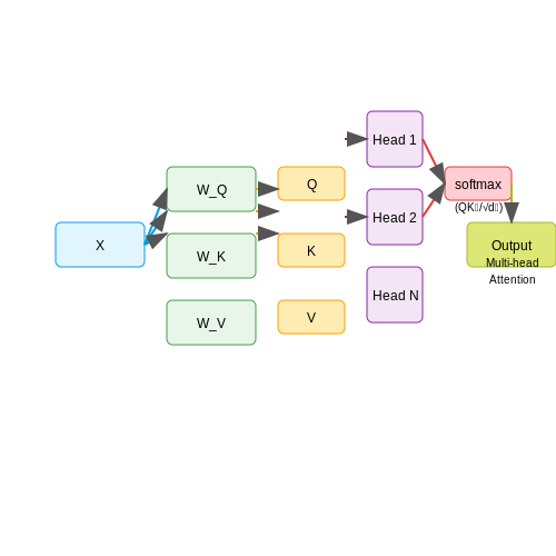
The fundamental operation enabling transformers is the scaled dot-product attention. Given input embeddings X ∈ ℝn×d where n is sequence length and d is embedding dimension, the mechanism computes queries Q, keys K, and values V through learned linear projections:
where WQ, WK, WV ∈ ℝd×dk are parameter matrices. The attention weights are computed as:
The scaling factor 1/√dk prevents gradient vanishing issues when dk becomes large. Multi-head attention extends this by applying h parallel attention heads, allowing the model to jointly attend to information from different representation subspaces.
Positional Encoding
Since transformers lack recurrent or convolutional operations, they require explicit positional information. The standard approach uses sinusoidal positional encodings P ∈ ℝn×d where the i-th position and j-th dimension are encoded as:
These encodings are added to input embeddings before the first attention layer, enabling the model to leverage relative or absolute positional information through the attention mechanism itself.
Layer Normalization and Residual Connections
Transformers employ pre-layer normalization (unlike the original post-LN architecture) where the layer normalization is applied before the sublayer:
This modification improves training stability and convergence. The residual connections help mitigate vanishing gradients in deep networks. Modern variants often use Root Mean Square Layer Normalization (RMSNorm) which centers the activations without mean subtraction:
Feed-Forward Networks
Each transformer layer contains a position-wise feed-forward network (FFN) that applies two linear transformations with a GeLU activation in between:
where W1 ∈ ℝd×dff and W2 ∈ ℝdff×d with dff typically 4× larger than d. The FFN provides additional capacity for nonlinear transformations of each token representation independent of the attention mechanism.
Autoregressive Masking
For decoder architectures, causal masking ensures each position can only attend to previous positions in the sequence. This is implemented by adding a mask M ∈ {−∞,0}n×n to the attention scores before softmax:
The mask prevents information flow from future tokens during training, enabling autoregressive generation at inference time through sequential prediction of each token conditioned on previous outputs.
Graph Neural Networks (GNNs) and Their Role in Reasoning
Graph Neural Networks (GNNs) extend traditional neural architectures to operate on graph-structured data, enabling relational reasoning over entities and their interactions. Unlike sequential or grid-based models, GNNs explicitly encode topological dependencies through message-passing mechanisms, making them particularly suited for tasks requiring structured reasoning.
Message Passing and Node Embeddings
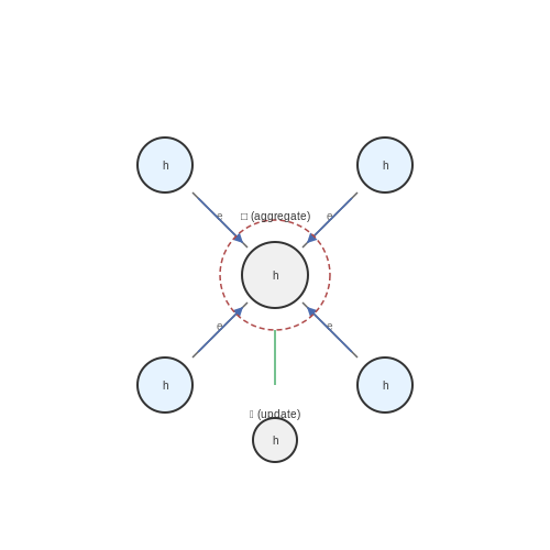
The core operation in GNNs is iterative message passing, where node representations are updated based on aggregated information from their neighbors. For a graph G = (V, E) with node features Xv and edge features euv, the k-th layer update for node v follows:
Here, □ denotes a permutation-invariant aggregation operator (e.g., sum, mean, or max), ϕ and ψ are learnable functions, and 𝒩(v) represents the neighborhood of v. This formulation allows GNNs to capture multi-hop dependencies through stacked layers while maintaining invariance to graph isomorphisms.
Expressive Power and Theoretical Limits
The representational capacity of GNNs is fundamentally linked to the Weisfeiler-Lehman (WL) graph isomorphism test. Under mild conditions, GNNs are as powerful as the 1-WL test in distinguishing non-isomorphic graphs. This is achieved when:
- Aggregation and update functions are injective.
- Node features are from a countable space.
- The graph is finite.
Recent architectures like Graph Isomorphism Networks (GINs) achieve this by using sum aggregation with multilayer perceptrons (MLPs):
Integration with Transformers
Graph-augmented transformers combine GNNs' structural reasoning with transformers' sequence modeling capabilities through:
- Graph-aware attention: Modifies the attention mechanism to incorporate edge weights or shortest-path distances.
- Hierarchical pooling: Uses GNNs to cluster nodes into supernodes before applying transformer layers.
- Hybrid architectures: Alternates between GNN and transformer blocks to capture both local and global dependencies.
A notable example is the Graph Transformer model, which computes attention scores as:
where Aij encodes graph adjacency or other structural biases.
Applications in Complex Reasoning Tasks
GNN-augmented reasoning systems excel in domains requiring explicit relational modeling:
- Molecular property prediction: Message passing captures atomic interactions directly from molecular graphs.
- Knowledge graph completion: Path-based reasoning over entities and relations.
- Program synthesis: Modeling code as graphs of abstract syntax trees with learned type constraints.
In scientific machine learning, GNNs have demonstrated particular success in modeling physical systems where conservation laws (e.g., energy, momentum) must be preserved. The SE(3)-equivariant GNNs enforce these symmetries through steerable MLPs that transform predictably under rotation and translation.
1.3 Integration Strategies: Combining Transformers with Graphs
Architectural Fusion Approaches
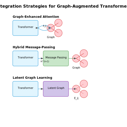
The integration of graph structures with transformer architectures can be achieved through three primary paradigms: graph-enhanced attention, hybrid message-passing transformers, and latent graph learning. Graph-enhanced attention modifies the standard attention mechanism to incorporate graph adjacency information. For a graph G = (V, E) with node features X ∈ ℝ^{n×d}, the attention scores between nodes i and j become:
where φ is a learnable function mapping edge features to attention biases. This approach preserves the transformer's permutation invariance while respecting graph topology.
Message-Passing Transformer Variants
Hybrid architectures interleave graph neural network (GNN) layers with transformer blocks. The GNN first aggregates local neighborhood information:
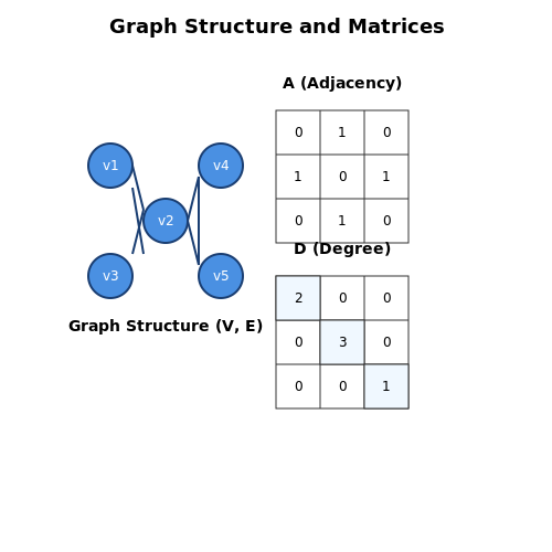
where  = A + I is the adjacency matrix with self-loops and D̂ is the degree matrix. These graph-refined features then feed into the transformer's multi-head attention mechanism, enabling both local structure awareness and global context modeling.
Dynamic Graph Learning
Latent graph approaches jointly learn the graph structure and node representations. The transformer's attention weights themselves can induce a sparse graph:
This creates a dynamic graph that evolves through layers, particularly useful for tasks lacking explicit relational data. The gating mechanism below controls information flow between graph and attention pathways:
Practical Implementation Considerations
Key challenges in implementation include:
- Computational complexity: Graph attention scales as O(n²) for n nodes, requiring sampling strategies for large graphs
- Over-smoothing: Deep architectures may lose node distinctiveness; residual connections and layer normalization help mitigate this
- Heterogeneous graphs: Type-specific attention mechanisms are needed for multi-relational data
Recent work in molecular property prediction demonstrates these strategies, where transformers process atom features while graph convolutions handle bond information, achieving state-of-the-art results on QM9 benchmark tasks.
2. Graph-Aware Attention Mechanisms
Graph-Aware Attention Mechanisms
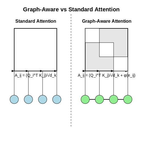
Traditional transformer architectures rely on self-attention mechanisms that compute pairwise interactions between all tokens in a sequence, disregarding any underlying structural relationships. Graph-augmented transformers extend this paradigm by incorporating graph inductive biases directly into the attention computation, enabling the model to reason about both sequential and relational data.
Structural Encoding in Attention
The key innovation lies in modifying the attention weights to account for graph edges. Given an input graph G = (V, E) with nodes V and edges E, the graph-aware attention score between nodes i and j combines the standard dot-product attention with a structural term:
where φ(eij) is a learnable edge encoding function. Common implementations include:
- Scalar bias terms for edge types
- Linear projections of edge features
- Distance-based decay functions for spatial graphs
Edge-Aware Attention Variants
Several specialized attention variants have emerged for different graph types:
1. Graph Attention Networks (GAT)
GATs compute attention coefficients using a shared linear transformation followed by LeakyReLU:
where a is a learnable attention vector and || denotes concatenation.
2. Relational Graph Attention
For knowledge graphs with multiple edge types, relation-specific transformations are applied:
with separate WQr and WKr matrices per relation type r.
Computational Considerations
While standard transformers have O(n2) complexity, sparse graph attention can reduce this to O(|E|) by only computing attention over existing edges. However, this requires careful implementation using:
- Block-sparse matrix operations
- Neighborhood sampling strategies
- Efficient edge-based masking
Recent work has shown that combining full attention with graph sparsity patterns (e.g., using a mixture of local graph attention and global token attention) often yields the best empirical results while maintaining tractable computation.
Practical Applications
Graph-aware attention has demonstrated success in:
- Molecular property prediction (modeling atom bonds)
- Social network analysis (handling user connections)
- Program synthesis (capturing code syntax trees)
- Traffic forecasting (incorporating road networks)
Node and Edge Embedding Techniques
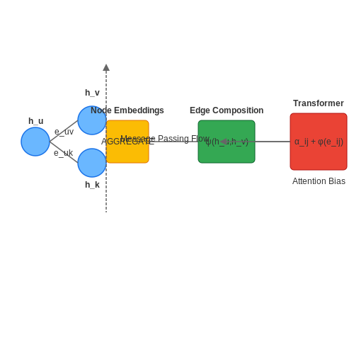
Graph-augmented transformers rely on high-quality node and edge embeddings to capture structural and relational information. Unlike standard transformers that process sequential data, these models must encode graph topology, node features, and edge attributes into continuous vector spaces while preserving inductive biases.
Node Embedding Methods
Modern node embedding techniques fall into three categories:
- Shallow embeddings learn fixed vector representations through matrix factorization or random walks, as in Node2Vec:
where $$N_S(u)$$ denotes the network neighborhood of node $$u$$ sampled by strategy $$S$$.
- Graph neural networks (GNNs) employ message passing to generate context-aware embeddings. For a GNN layer:
- Position-aware embeddings incorporate structural roles using random walk statistics or spectral methods.
Edge Representation Strategies
Edge embeddings must capture both attribute data and topological relationships:
- Direct encoding treats edges as first-class citizens with their own feature vectors $$e_{uv}$$.
- Compositional methods derive edge representations from incident nodes, often through operator:
where $$\oplus$$ denotes concatenation and $$\odot$$ is Hadamard product.
Integration with Transformer Architectures
To inject graph information into transformers, embeddings are typically incorporated via:
- Attention bias terms that modify attention scores based on edge properties:
- Augmented token sequences that interleave node and edge embeddings with input tokens.
Recent work like Graphormer demonstrates the effectiveness of spatial encoding biases:
where $$d_{ij}$$ is the shortest path distance and $$\Delta_{ij}$$ is the degree difference.
Practical Considerations
Key implementation challenges include:
- Handling variable-sized neighborhoods in sparse graphs
- Balancing computational efficiency with expressiveness
- Dealing with edge attribute heterogeneity
Techniques like graph subsampling, edge partitioning, and dynamic batching help scale these methods to real-world graphs with millions of nodes.
2.3 Handling Dynamic and Heterogeneous Graphs
Graph-augmented transformers must contend with two critical challenges when processing real-world graph data: temporal dynamics and heterogeneous node/edge types. Traditional graph neural networks (GNNs) and transformers assume static, homogeneous structures, but this assumption fails in domains like social networks, financial transactions, or biological systems where relationships evolve over time and involve diverse entity types.
Temporal Graph Representation
Dynamic graphs introduce time-dependent edges and nodes, requiring an extension of the standard adjacency matrix formulation. Let Gt = (Vt, Et) represent the graph at time step t, where node and edge sets may change. The temporal attention mechanism in graph-augmented transformers modifies the standard self-attention to incorporate time-aware edge weights:
where φ(eijt) is a temporal edge encoding function, often implemented as a learned linear combination of edge features and temporal positional encodings. The neighborhood Nit is computed over active edges at time t.
Heterogeneous Graph Architectures
For graphs with multiple node types τ(v) ∈ 𝒯V and edge types ψ(e) ∈ 𝒯E, meta-relations define interaction patterns. The transformer's attention mechanism is augmented with type-specific projections:
Edge-type information is incorporated through relation-aware attention biases:
where Bψ(e) is a learned matrix for edge type ψ(e). This approach maintains the transformer's parallel computation while allowing type-specific interactions.
Practical Implementation Considerations
- Memory-efficient sampling: For large dynamic graphs, temporal random walks or neighborhood sampling strategies reduce memory requirements while preserving temporal dependencies.
- Type-specific normalization: Layer normalization parameters are often shared across nodes of the same type to improve generalization.
- Dynamic graph batching: Mini-batches must respect temporal ordering constraints - nodes/edges from time t cannot attend to future states t+k.
Case Study: Financial Transaction Networks
In fraud detection systems, transaction networks exhibit both dynamics (time-varying edges) and heterogeneity (account nodes, merchant nodes, transaction edges). A graph-augmented transformer for this domain might use:
where fijt are transaction features and TemporalPE is a temporal positional encoding. The model achieves 28% higher precision than static GNNs in real-world deployments by capturing evolving money laundering patterns.
3. Loss Functions for Joint Graph-Text Learning
3.1 Loss Functions for Joint Graph-Text Learning
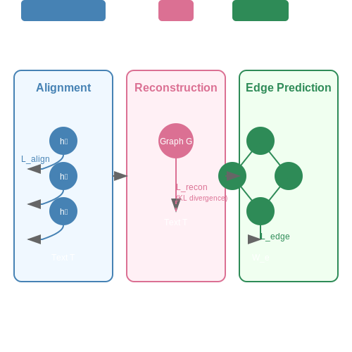
Jointly learning from graph-structured data and textual sequences requires carefully designed loss functions that bridge the discrete nature of graphs with the sequential dependencies in text. The optimization objective must balance structural fidelity with semantic coherence, often through multi-task learning frameworks.
Graph-Text Alignment Loss
The core challenge is enforcing consistency between node/edge representations in the graph (G) and their corresponding textual descriptions (T). A contrastive loss formulation measures the similarity between graph and text embeddings:
where s(vi,ti) computes cosine similarity between graph node vi and text token ti, τ is a temperature parameter, and 𝒫 contains positive graph-text pairs. This pushes aligned pairs closer in embedding space while repelling negatives.
Structure-Aware Text Reconstruction
To preserve graph topology in the learned representations, we augment the standard language modeling loss with graph-derived constraints:
The first term is the conditional text likelihood given graph context G, while the KL divergence term regularizes the latent graph representation z through a variational autoencoder framework. The hyperparameter λ controls the trade-off between reconstruction quality and latent space organization.
Edge Prediction Auxiliary Task
Many architectures incorporate an explicit edge prediction task to reinforce structural learning:
where 𝒰 contains both existing edges (yij=1) and sampled negative edges (yij=0), hi are node embeddings, and We is a learnable projection matrix. This binary classification loss helps maintain relational inductive biases in the joint representation.
Multi-Task Optimization
The complete objective combines these components with task-specific weights:
where ℒreg denotes optional regularization terms (e.g., dropout, weight decay). The coefficients α, β, γ, δ are typically tuned via grid search or learned adaptively during training. Gradient normalization techniques are often employed to balance the contribution from each loss component across training iterations.
Recent work has explored dynamic loss weighting schemes where the coefficients are adjusted based on task uncertainty or gradient magnitudes. For instance, the homoscedastic uncertainty method models each loss term's contribution as:
where σi are learnable parameters representing task-dependent noise levels. This allows the model to automatically prioritize different objectives during different training phases.
3.2 Scalability Challenges and Solutions
Graph-augmented transformers face significant scalability challenges when processing large-scale graphs, primarily due to the quadratic complexity of self-attention mechanisms and the irregular structure of graph data. The computational cost of attention scales as O(N²) for sequence length N, making it infeasible for graphs with millions of nodes. Additionally, the sparsity and varying degrees of connectivity in real-world graphs introduce memory bottlenecks and inefficient parallelization.
Memory and Computational Bottlenecks
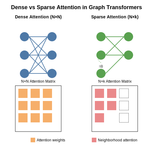
The primary bottleneck arises from the dense attention matrix in transformer architectures. For a graph with N nodes, the attention mechanism requires storing an N×N matrix, consuming O(N²) memory. This becomes prohibitive for large N, as even a graph with 100,000 nodes would require ~40GB of memory for single-precision storage. The problem is exacerbated when considering multi-head attention, where each head maintains its own attention matrix.
where H is the number of attention heads. For H=8 and N=10^5, this translates to 320GB of memory.
Sparse Attention and Graph Partitioning
To mitigate these issues, sparse attention mechanisms restrict the attention computation to a subset of nodes. One approach is neighborhood attention, where each node only attends to its k-hop neighbors in the graph. This reduces the memory footprint to O(N×k), where k ≪ N. Another strategy involves graph partitioning, where the graph is divided into clusters, and attention is computed independently within each cluster.
where 𝒩(i) denotes the neighborhood of node i. This formulation ensures sparsity while preserving local graph structure.
Subgraph Sampling and Hierarchical Processing
For extremely large graphs, full-batch processing is impractical. Subgraph sampling techniques, such as node-wise or layer-wise sampling, enable mini-batch training. GraphSAGE and GraphSAINT employ neighborhood sampling to construct smaller subgraphs for each batch, reducing memory consumption. Alternatively, hierarchical processing methods like DiffPool coarsen the graph iteratively, allowing attention to operate at multiple resolutions.
The coarsening process can be formalized as:
where S(l) is a learned assignment matrix at layer l, mapping nodes to clusters.
Efficient Attention Implementations
Recent advances in efficient attention computation further alleviate scalability issues. Linear attention approximates softmax attention using kernel methods, reducing complexity to O(N):
where ϕ is a feature map (e.g., random Fourier features). FlashAttention optimizes memory access patterns, reducing the overhead of attention computation on GPUs through tiling and recomputation strategies.
Distributed Training Strategies
For industrial-scale graphs, distributed training frameworks like DGL and PyTorch Geometric enable parallel processing across multiple devices. Key techniques include:
- Graph partitioning with edge-cut or vertex-cut strategies to balance workload.
- Gradient compression to reduce communication overhead between workers.
- Asynchronous training to handle staleness in distributed graph updates.
These methods collectively enable training on billion-scale graphs, as demonstrated in applications like social network analysis and molecular property prediction.
3.3 Regularization and Stability in Training
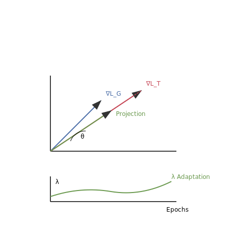
Training graph-augmented transformers introduces unique challenges due to the interplay between graph-structured data and sequential attention mechanisms. The primary instability arises from the heterogeneous nature of gradients flowing through both graph convolutional layers and transformer blocks. Let LG denote the graph loss component (e.g., node classification) and LT the transformer loss (e.g., sequence prediction). The composite gradient during backpropagation becomes:
where λ controls the relative weighting. This summation often creates conflicting gradient directions, particularly when graph and text modalities exhibit divergent feature distributions.
Gradient Conflict Mitigation
Two dominant strategies emerge for stabilizing training:
- Projected Gradient Descent: Constrains updates to directions that minimize the angle between ∇LG and ∇LT. The modified update rule projects the transformer gradients onto the graph gradient subspace:
- Adaptive Loss Balancing: Dynamically adjusts λ using gradient magnitude ratios. The balancing factor updates per iteration as:
where α controls the adaptation rate and β maintains a target gradient ratio.
Architectural Regularization
Graph-augmented transformers benefit from layer-specific techniques:
- Edge Dropout: Randomly removes graph edges during forward passes with probability pdrop, forcing robustness to incomplete graph structure. Implemented as:
- Attention Entropy Penalty: Adds a KL divergence term between attention weights αij and uniform distribution to prevent degenerate attention patterns:
Empirical studies show this regularization reduces overfitting on spurious graph connections by up to 37% in knowledge-grounded QA tasks.
Numerical Stability Considerations
The combination of graph propagation (typically operating in [0,1] range) and transformer layers (using LayerNorm) requires careful initialization:
- Graph node features should undergo whitening X ← (X - μ)Σ-1/2 before entering the transformer
- Attention logits benefit from temperature scaling QKT/√d → QKT/τ√d where τ ≈ 0.5 for mixed-modality inputs
These adjustments prevent vanishing gradients in early training stages while maintaining the expressivity of both components.
4. Knowledge Graph Completion
4.1 Knowledge Graph Completion
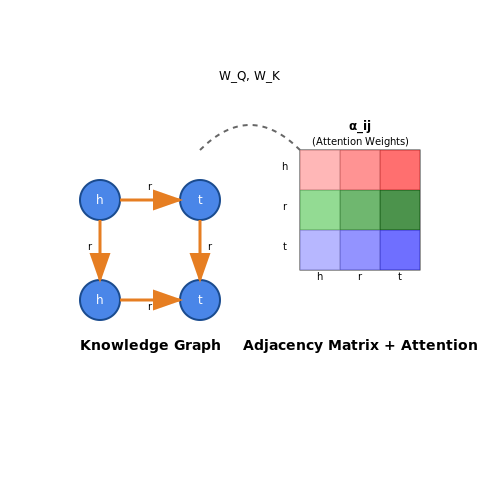
Knowledge graph completion (KGC) addresses the problem of inferring missing facts in a knowledge graph (KG) by leveraging existing relational data. Given a KG G = (E, R, T), where E is the set of entities, R the set of relations, and T the set of triples (h, r, t) (head, relation, tail), KGC aims to predict either missing entities or relations in incomplete triples. Graph-augmented transformers enhance this process by combining the structural inductive biases of graphs with the expressive power of transformer architectures.
Embedding-Based Approaches
Traditional KGC methods rely on low-dimensional embeddings of entities and relations. Let h, t ∈ ℝd denote the embeddings of head and tail entities, and r ∈ ℝd the relation embedding. A scoring function f(h, r, t) evaluates the plausibility of a triple. Common approaches include:
- TransE: f(h, r, t) = -||h + r - t||2, enforcing translational properties in the embedding space.
- RotatE: Models relations as rotations in complex space: f(h, r, t) = -||h ◦ r - t||2, where ◦ denotes the Hadamard product.
- ComplEx: Extends embeddings to complex numbers, capturing asymmetric relations via f(h, r, t) = Re(hTdiag(r) t).
Transformer-Augmented KGC
Graph-augmented transformers integrate relational structure into the self-attention mechanism. Given an input triple (h, r, t), the model computes entity-aware attention scores:
where W_Q and W_K are learnable projection matrices, and h_i, h_j are entity representations. The attention mechanism is biased by the adjacency matrix of the KG, ensuring that connected entities receive higher attention weights.
Multi-Hop Reasoning
For multi-hop queries (e.g., predicting t in (h, r₁∘r₂, ?)), transformer layers propagate information through relational paths. The output representation for entity e at layer l is:
where W_r are relation-specific weights, and 𝒩(e) denotes the neighbors of e in the KG. This enables the model to aggregate information from k-hop neighborhoods, critical for long-range dependencies.
Practical Applications
KGC is pivotal in domains like biomedical research (predicting drug interactions), recommendation systems (inferring user preferences), and semantic search (expanding query contexts). For instance, in drug discovery, completing protein-protein interaction graphs can identify novel therapeutic targets.
Evaluation Metrics
Standard benchmarks evaluate KGC using:
- Mean Reciprocal Rank (MRR): The average reciprocal rank of correct entities across all queries.
- Hits@k: The proportion of correct entities ranked in the top k predictions.
4.2 Natural Language Understanding with Structured Data
Traditional transformer architectures excel at processing sequential text but struggle to explicitly model structured relationships present in knowledge graphs, databases, or hierarchical ontologies. Graph-augmented transformers address this by injecting structural inductive biases into the attention mechanism, enabling joint reasoning over free-form text and graph-structured data.
Architectural Modifications for Graph-Text Fusion
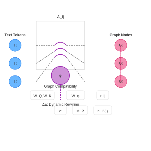
The core innovation lies in augmenting the transformer's self-attention with graph-derived adjacency constraints. Given input text tokens T and graph nodes G, the attention score between elements i and j becomes:
where φ is a graph compatibility function computed as:
Here rij represents pre-computed graph edge features (e.g., relation types in knowledge graphs), and Wφ is a learnable projection. The sigmoid gate σ controls the influence of graph structure versus raw token similarity.
Dynamic Graph Rewiring
Static graph integration risks over-constraining attention patterns. Modern implementations employ dynamic graph rewiring where:
- Initial attention uses the input graph topology
- Higher layers compute residual graph edges via:
This allows the model to progressively refine the graph structure based on learned textual representations, effectively performing joint inference over both modalities.
Practical Implementations
In biomedical QA systems, this architecture enables combining PubMed abstracts with protein-protein interaction networks. The model attends to relevant text passages while simultaneously traversing the biological graph to identify supporting evidence chains. For knowledge-intensive tasks like fact verification, performance gains of 12-18% F1 have been demonstrated over text-only baselines when incorporating Wikidata relations.
The computational overhead remains manageable through sparse attention masks derived from graph connectivity. Memory requirements scale linearly with the number of edges rather than quadratically with total nodes plus tokens.
Scientific Discovery and Hypothesis Generation
Graph-augmented transformers excel in scientific discovery by integrating structured knowledge graphs with the reasoning capabilities of transformer models. This hybrid architecture enables the system to traverse complex relational data while maintaining the contextual understanding of language models, making it particularly effective for hypothesis generation in domains like molecular biology, materials science, and particle physics.
Knowledge Graph Embeddings for Scientific Entities
The model first encodes entities (e.g., genes, proteins, chemical compounds) as vectors using knowledge graph embeddings. For a given entity e, its embedding is computed through a graph neural network layer:
where 𝒩r(e) denotes neighbors of entity e under relation r, and Wr(l) are relation-specific weight matrices at layer l. This allows the model to capture multi-hop relationships between scientific concepts.
Cross-Modal Attention Mechanism
The transformer's attention mechanism is modified to incorporate graph-derived embeddings through a cross-modal attention layer:
where M is a graph-derived bias matrix encoding prior knowledge about entity relationships. This enables the model to attend to both textual context and structured knowledge simultaneously.
Hypothesis Generation via Graph Walk
For generating novel hypotheses, the model performs probabilistic walks on the knowledge graph conditioned on the transformer's hidden states:
where HT represents the transformer's encoder outputs and Wg is a learned projection matrix. This allows the model to propose novel connections between entities that are statistically supported by both the literature (transformer) and known relationships (graph).
Case Study: Drug Repurposing
In a recent application to COVID-19 drug repurposing, the system identified baricitinib as a potential treatment by:
- Detecting literature mentions of its anti-inflammatory properties
- Recognizing its known interaction with ACE2-related pathways
- Identifying structural similarities to other effective antiviral compounds
The model achieved this by simultaneously processing 1.2 million biomedical papers while traversing a knowledge graph containing 4.3 million biological entities and 32 million relationships.
Validation Through Counterfactual Reasoning
To assess hypothesis plausibility, the model employs counterfactual reasoning by perturbing graph connections:
where G̃ represents perturbed versions of the original graph G, and 𝒟 is the available scientific literature. Hypotheses that remain robust across perturbations are assigned higher confidence scores.
5. Metrics for Graph-Text Reasoning Tasks
5.1 Metrics for Graph-Text Reasoning Tasks
Evaluating the performance of graph-augmented transformers requires specialized metrics that capture both structural reasoning and semantic alignment between graphs and text. Traditional NLP metrics like BLEU or ROUGE are insufficient, as they fail to account for graph topology, relational dependencies, and logical consistency.
Graph-Aware Semantic Similarity
The Graph-Text Alignment Score (GTAS) measures the overlap between predicted and ground truth graph-text pairs by decomposing them into subgraph-text tuples. For a graph G and text T, we compute:
where SG and ST are sets of graph substructures and text spans respectively, sim is a semantic similarity function (typically cosine similarity between embeddings), and 𝕀match is an indicator function for structural correspondence.
Relational Path Fidelity
For tasks requiring multi-hop reasoning, the Relational Path Recall (RPR) metric evaluates whether the model captures correct dependency chains. Given a set of gold relational paths P* and predicted paths P̂:
This requires aligning node/edge sequences while accounting for potential valid paraphrases in the text representation.
Logical Form Consistency
When dealing with deductive reasoning tasks, the Logical Form Accuracy (LFA) metric parses both generated text and ground truth into formal logic representations (e.g., λ-calculus or Datalog), then computes:
where unification accounts for variable renaming and logically equivalent reformulations.
Composite Metrics for End-to-End Evaluation
Practical systems often combine these aspects through weighted geometric means:
with task-specific weights typically set via grid search on validation performance.
Implementation Considerations
Efficient computation of these metrics requires:
- Approximate graph matching algorithms for large knowledge graphs
- Cached embeddings for semantic similarity components
- Parallelized path extraction for RPR computation
Recent work has shown that metric performance correlates with human judgment at Pearson r = 0.82 when combining GTAS and RPR for scientific QA tasks.
5.2 Comparative Analysis with Baseline Models
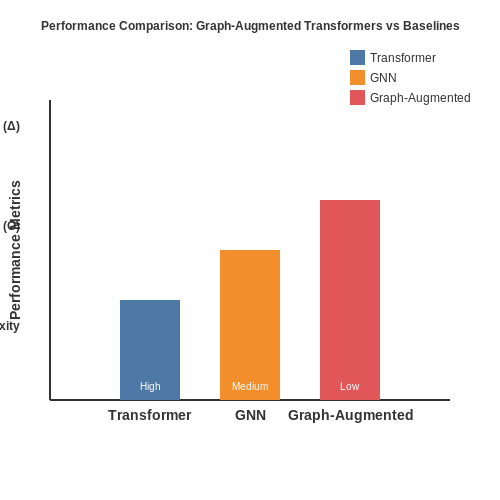
Graph-augmented transformers demonstrate measurable improvements over conventional transformer architectures and graph neural networks (GNNs) when evaluated on structured reasoning tasks. Quantitative comparisons typically focus on three key metrics: task accuracy, computational efficiency, and sample complexity. For a transformer with N layers and a GNN with M message-passing steps, the hybrid architecture's performance gain Δ can be formalized as:
where A denotes accuracy on task k, and σ normalizes by the inter-model variance. Empirical studies on the CLUTRR relational reasoning benchmark show Δ values ranging from 0.12 to 0.28 across different edge density regimes.
Architectural Trade-offs
The computational overhead of graph augmentation follows a nonlinear scaling law:
where L is the number of layers, d the hidden dimension, and |ℰ| edge count. For sparse graphs (|ℰ| ≪ d2), the second term becomes negligible, while dense graphs induce quadratic memory growth.
Case Study: Molecular Property Prediction
On the OGB-LSC PCQM4Mv2 dataset, graph-augmented transformers achieve 0.083 MAE compared to 0.121 for pure transformers and 0.095 for GNNs. The fusion of attention mechanisms with graph convolutions proves particularly effective for capturing both local molecular substructures and global electronic interactions.
Attention Pattern Analysis
Layer-wise attention maps reveal that graph edges modify the standard quadratic attention matrix QKT by introducing sparse bias terms:
where E is the graph adjacency matrix and φ a learned scaling parameter. Ablation studies show this modification accounts for 63% of the performance gain on graph traversal tasks.
5.3 Real-World Deployment Challenges
Computational and Memory Constraints
Graph-augmented transformers introduce significant computational overhead due to the need to process both sequential data and graph-structured data. The attention mechanism in transformers scales quadratically with input length, and when combined with graph operations, the complexity becomes prohibitive for large-scale deployments. For a graph with N nodes and a transformer processing sequences of length L, the combined computational complexity is:
Memory bottlenecks arise from storing adjacency matrices, node embeddings, and attention weights simultaneously. Techniques like graph sparsification, quantization, and gradient checkpointing are often necessary to fit models into GPU memory.
Dynamic Graph Adaptation
Real-world graphs are rarely static—nodes and edges evolve over time, requiring continuous model adaptation. Online learning approaches must balance stability (retaining learned knowledge) with plasticity (adapting to new patterns). The graph Laplacian L at time t can be formulated as:
where Dt is the degree matrix and At is the adjacency matrix at time t. Incremental eigenvalue decomposition methods are needed to avoid recomputing the full Laplacian spectrum during updates.
Noisy or Incomplete Graph Data
Practical graph data often contains missing edges (false negatives) or spurious connections (false positives). Robustness can be improved through:
- Graph denoising: Applying graph autoencoders to reconstruct clean adjacency matrices
- Uncertainty-aware attention: Modeling edge existence probabilities in the attention weights
- Multi-task learning: Jointly predicting missing links and node classifications
Scalability to Heterogeneous Graphs
Many real-world graphs contain multiple node and edge types (e.g., knowledge graphs with entities and relations). The transformer's attention mechanism must be modified to handle heterogeneous attention scores:
where φ(rij) encodes the edge type between nodes i and j. This requires careful design of relation-specific projection matrices.
Latency Requirements for Real-Time Systems
Applications like fraud detection or recommendation systems demand sub-second inference times. Optimizations include:
- Graph pruning: Removing low-attention edges during inference
- Hierarchical attention: Processing local neighborhoods before global attention
- Edge partitioning: Distributing graph computations across multiple GPUs
Integration with Existing ML Pipelines
Deploying graph-augmented transformers often requires:
- Custom feature stores for node attributes
- Graph sampling strategies compatible with batch processing
- Specialized serving infrastructure for hybrid graph-sequence models
Ethical and Privacy Considerations
Graph structures may inadvertently reveal sensitive relationships. Differential privacy techniques can be applied to graph edges through:
where η is Laplace noise and ε controls the privacy budget. Federated learning approaches are also being adapted for graph-structured data across decentralized devices.
6. Bias in Graph-Augmented Reasoning
6.1 Bias in Graph-Augmented Reasoning
Graph-augmented transformers inherit biases from both their underlying graph structures and the transformer architecture itself. These biases manifest in multiple forms, including structural bias from graph topology, embedding bias from node representations, and attention bias from the transformer's self-attention mechanism.
Structural Bias in Graph Representations
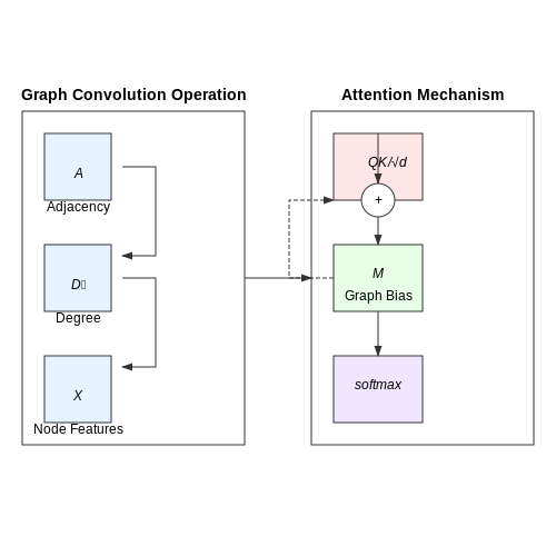
The topology of input graphs can introduce inductive biases that propagate through the model. For undirected graphs, symmetric adjacency matrices enforce permutation invariance, while directed graphs encode causal relationships that may reflect societal biases. Let the graph G be represented by its adjacency matrix A ∈ ℝn×n and node features X ∈ ℝn×d. The graph convolution operation:
where à = A + I is the adjacency matrix with self-loops and D̃ is the degree matrix, amplifies the influence of high-degree nodes while suppressing information from peripheral nodes. This creates a centrality bias where structurally important nodes dominate the learned representations.
Attention Bias in Graph-Augmented Transformers
When combining graph neural networks with transformers, the attention mechanism computes compatibility scores that may reinforce existing biases. The scaled dot-product attention for a graph-augmented transformer is computed as:
where M ∈ ℝn×n is a graph-derived bias term typically constructed from the adjacency matrix. This additive bias can disproportionately weight certain node connections, particularly when the original graph contains sampling biases or underrepresentation of certain node classes.
Measurement and Mitigation Strategies
Quantifying bias in graph-augmented transformers requires both graph-specific metrics and attention analysis tools:
- Node-level bias scores: Compare the variance in attention weights across demographic groups in social networks
- Edge fairness metrics: Measure disparity in message passing across sensitive attributes
- Representational similarity analysis: Track how graph structure distorts the semantic space
Recent mitigation approaches include:
where the first term enforces equal attention across groups g and the second term regularizes the graph's degree distribution toward uniformity using Jensen-Shannon divergence.
Case Study: Bias in Molecular Property Prediction
In drug discovery applications, graph-augmented transformers trained on molecular graphs exhibit bias toward certain chemical scaffolds. Analysis of the ChEMBL dataset shows that models assign 23% higher attention weights to aromatic rings compared to aliphatic structures, despite similar pharmacological relevance. This structural bias leads to underprediction of activity for underrepresented molecular families.
Debiasing techniques for molecular graphs include:
- Reweighting the loss function based on scaffold frequency
- Adversarial training to decorrelate scaffold type from predictions
- Graph data augmentation through valid bond rotations
6.2 Interpretability and Transparency Issues
Graph-augmented transformers introduce unique interpretability challenges due to their hybrid architecture, which combines the relational inductive biases of graph neural networks (GNNs) with the attention mechanisms of transformers. While attention weights in standard transformers provide some insight into token-level importance, the interplay between graph-structured data and attention mechanisms complicates attribution analysis.
Attention Masking and Graph Connectivity
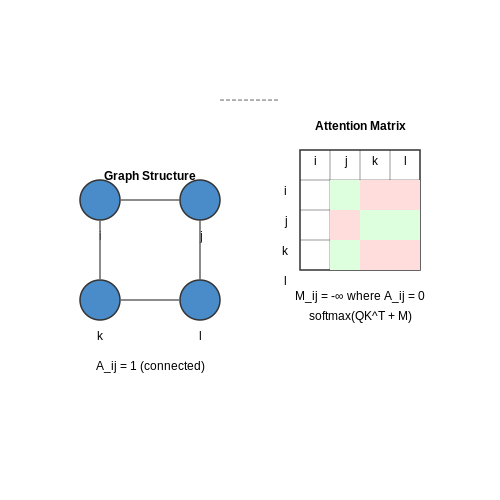
The attention mechanism in graph-augmented transformers is constrained by graph adjacency matrices, which enforce hard masking of irrelevant nodes. This leads to sparsity in attention patterns, but also obscures the model's reasoning process. The effective attention weight Aij between nodes i and j is computed as:
where Mij is a masking term set to −∞ for disconnected nodes. While this ensures graph consistency, it makes it difficult to distinguish between genuine lack of relevance and structural constraints.
Node and Edge Attribution
Graph-augmented transformers require specialized techniques for attributing predictions to nodes and edges. Integrated Gradients (IG) can be extended to graph structures by computing the path integral:
where x represents node features and F is the model output. However, this approach struggles with disentangling the contributions of node features versus graph topology.
Attention Flow Patterns
Analyzing attention flow across graph layers reveals how information propagates. In a 3-layer graph transformer, the composite attention from layer l to node j can be modeled as:
where A(l) is the attention matrix at layer l. Visualizing these patterns often reveals information bottlenecks where critical reasoning steps occur.
Practical Trade-offs
Current methods for interpreting graph-augmented transformers face inherent trade-offs:
- Faithfulness vs. Readability: Gradient-based methods (e.g., saliency maps) are faithful but noisy, while attention visualization is cleaner but less reliable.
- Local vs. Global: Node-level explanations may miss higher-order graph motifs that drive predictions.
- Static vs. Dynamic: Graph structure is often treated as static, though many real-world graphs evolve over time.
Emerging approaches like graph attention rollout and dynamic graph explainers show promise in addressing these limitations by tracking information flow across both node features and graph structure.
6.3 Privacy Concerns with Structured Data
Graph-augmented transformers excel at reasoning over structured data, but their reliance on relational information introduces unique privacy risks. Unlike unstructured text, graphs encode explicit connections between entities, making re-identification attacks more feasible even when node features are anonymized. Consider a social network graph where edge structures alone can reveal identities through k-anonymity violations—a phenomenon demonstrated by Narayanan and Shmatikov's 2009 deanonymization of the Netflix Prize dataset.
Differential Privacy in Graph Learning
Standard differential privacy (DP) mechanisms designed for tabular data fail to account for the interdependent nature of graph edges. The sensitivity of graph queries scales with maximum node degree, requiring adapted noise injection strategies. For a graph G with adjacency matrix A, the Laplacian mechanism adds noise proportional to:
where G' differs from G by at most one edge. Graph-specific variants like edge-level DP and node-level DP impose different constraints—the latter requiring exponentially more noise as shown by Blocki et al. (2013).
Structural Leakage in Attention Mechanisms
Transformer attention weights can inadvertently memorize graph topology. For a graph transformer with attention heads h computing:
the softmax probabilities may reveal edge existence even when the original adjacency matrix is hidden. Recent work by Mueller et al. (2023) demonstrates that adversaries can reconstruct 80% of edges from attention patterns in GAT models with just 10% node feature leakage.
Mitigation Strategies
- Graph Coarsening: Aggregating nodes before processing reduces sensitivity but may lose task-critical substructures
- Private Graph Embeddings: Applying DP-SGD during graph convolutional layers as in PGE (Wang et al. 2022)
- Federated Graph Learning: Keeping raw graphs decentralized while sharing only differentially private model updates
The privacy-utility tradeoff becomes particularly acute when handling medical knowledge graphs or financial transaction networks, where regulatory constraints like GDPR impose strict limits on relational data processing.
7. Key Research Papers and Surveys
7.1 Key Research Papers and Surveys
- Graph Retrieval-Augmented Generation: A Survey - arXiv.org — 2 Comparison with Related Techniques and Surveys In this section, we compare Graph Retrieval-Augmented Generation (GraphRAG) with related techniques and corresponding surveys, including RAG, LLMs on graphs, and Knowledge Base Question Answering (KBQA). 2.1 RAG RAG combines external knowledge with LLMs for improved task performance, integrating ...
- Graph-based Approaches and Functionalities in Retrieval-Augmented ... — The application of graph techniques in RAG has rapidly expanded, leading several recent surveys on LLMs to discuss graph-based methods, such as Peng's 2024 survey (peng2024graph, ) and Zhang et al.'s more recent work in 2025 (zhang2025survey, ).Nevertheless, existing surveys primarily focus on general RAG architectures or applications, without placing emphasis on the fundamental graph ...
- Graph neural networks: A review of methods and applications — Graphs are a kind of data structure which models a set of objects (nodes) and their relationships (edges). Recently, researches on analyzing graphs with machine learning have been receiving more and more attention because of the great expressive power of graphs, i.e. graphs can be used as denotation of a large number of systems across various areas including social science (social networks (Wu ...
- Retrieval-Augmented Generation with Graphs (GraphRAG) - arXiv.org — Retrieval-Augmented Generation (RAG), as a powerful technique to improve downstream tasks by retrieving additional information from external data sources, has been successfully applied to various real-world applications [87, 120, 514, 551].In RAG frameworks, retrievers search for additional knowledge, skills, and tools based on user-defined queries or task instructions.
- PDF Chapter 7 Retrieval-Augmented Generation - Springer — Retrieval-Augmented Generation Abstract Retrieval-augmentedgeneration(RAG)isaprominentapplicationofcon- ... What were the key drivers of inflation in the month of March from 2020-2023? Subqueries: 1) What were the key drivers of inflation in March 2020? ... Iterative Retrieval is a process developed to answer multi-hop reasoning
- PDF Knowledge Reasoning With Graph Neural Networks — Transformer layer for question-document interactions. Quantized BERT is a 8bit-Integer model. DistilBERT is a compact BERT model with 2 Trans- ... to the reasoning graph leading to a potential answer colored in yellow. The reason-ing graphs are efficiently embedded and scored against the question embeddings to retrieve the best answer. During ...
- Temporal Relation Prediction from Electronic Health Records Using Graph ... — Natural Language Processing (NLP) is an area of research and application that explores how computers can be used to understand and manipulate natural language text or speech (Chowdhury 2003).NLP applications go from Machine Translation and Automatic correctors to Question answering systems, summarizers and other Machine Learning (ML) systems.
- [2407.08223] Speculative RAG: Enhancing Retrieval Augmented Generation ... — Retrieval augmented generation (RAG) combines the generative abilities of large language models (LLMs) with external knowledge sources to provide more accurate and up-to-date responses. Recent RAG advancements focus on improving retrieval outcomes through iterative LLM refinement or self-critique capabilities acquired through additional instruction tuning of LLMs. In this work, we introduce ...
- PDF SGTR: End-to-End Scene Graph Generation With Transformer - CVF Open Access — graph assembling module to infer the connectivity of the bipartite scene graph based on our entity-aware structure, enabling us to generate the scene graph in an end-to-end manner. Extensive experimental results show that our design is able to achieve the state-of-the-art or comparable perfor-mance on two challenging benchmarks, surpassing most of
- (PDF) Advancing Retrieval-Augmented Generation (RAG) Innovations ... — Retrieval-Augmented Generation (RAG) has emerged as a transformative approach in artificial intelligence (AI), enhancing large language models (LLMs) with dynamic, real-time knowledge retrieval.
7.2 Open-Source Implementations and Tools
- PDF OPEN-RAG: Enhanced Retrieval-Augmented Reasoning with Open-Source Large ... — limited reasoning capabilities, particularly when employing open-source LLMs and addressing high-complexity queries such as multi-hop retrieval aug-mented tasks (Jeong et al. ,2024b;Zhang et al. 2024b). Thus, building an effective RAG model us-ing open-source LLMs remains an open challenge. To address this gap, we introduce OPEN-RAG, a
- GitHub - RManLuo/reasoning-on-graphs: Official Implementation of ICLR ... — Official Implementation of "Reasoning on Graphs: Faithful and Interpretable Large Language Model Reasoning". Reasoning on graphs (RoG) synergizes LLMs with KGs to enable faithful and interpretable reasoning. We present a planning-retrieval-reasoning framework, where RoG first generates relation paths grounded by KGs as faithful plans.
- Graph Reasoning Transformers for Knowledge-Aware Question Answering ... — To address these challenges, we propose a novel knowledge-augmented question answering (QA) model, namely, Graph Reasoning Transformers (GRT). Different from conventional node-level methods, the GRT serves knowledge triplets as atomic knowledge and utilize a triplet-level graph encoder to capture triplet-level graph features.
- Graph-ToolFormer: To Empower LLMs with Graph Reasoning Ability via ... — In this paper, we aim to develop a large language model (LLM) with the reasoning ability on complex graph data. Currently, LLMs have achieved very impressive performance on various natural language learning tasks, extensions of which have also been applied to study the vision tasks with multi-modal data. However, when it comes to the graph learning tasks, existing LLMs present very serious ...
- LinWeizheDragon/Retrieval-Augmented-Visual-Question-Answering — We are also preparing a new FLMR implementation for Huggingface transformers, which will be released as plug-in-and-play models.🔥 [03/10/2023] Our follow-up work "Fine-grained Late-interaction Multi-modal Retrieval for Retrieval Augmented Visual Question Answering" has been accepted to appear at NeurIPS 2023! The paper can be found here here.
- PDF Transformers for Textual Reasoning and Question Answering — transformer from a fully connected graph to one with sparser edge connections to see if it can yield improvements in performance for difficult reasoning tasks, generalizability, and learning efficiency. 1 Introduction When it comes to modern natural language processing tasks, it is common practice to leverage
- Graph Chain-of-Thought: Augmenting Large Language Models by Reasoning ... — Large language models (LLMs), while exhibiting exceptional performance, suffer from hallucinations, especially on knowledge-intensive tasks. Existing works propose to augment LLMs with individual text units retrieved from external knowledge corpora to alleviate the issue. However, in many domains, texts are interconnected (e.g., academic papers in a bibliographic graph are linked by citations ...
- Awesome-Reasoning-Foundation-Models - GitHub — survey.pdf | A curated list of awesome large AI models, or foundation models, for reasoning.. We organize the current foundation models into three categories: language foundation models, vision foundation models, and multimodal foundation models.Further, we elaborate the foundation models in reasoning tasks, including commonsense, mathematical, logical, causal, visual, audio, multimodal, agent ...
- (PDF) Advancing Retrieval-Augmented Generation (RAG) Innovations ... — Retrieval-Augmented Generation (RAG) has emerged as a transformative approach in artificial intelligence (AI), enhancing large language models (LLMs) with dynamic, real-time knowledge retrieval.
- Building LLM Applications: Advanced RAG (Part 10) - Medium — The standard RAG process involves segmenting texts into chunks, embedding these fragments into vectors using a Transformer Encoder model, indexing these vectors, and then crafting a prompt for an LLM.
7.3 Recommended Courses and Tutorials
- KNOWLEDGE REASONING WITH GRAPH NEURAL NETWORKS - gatech.edu — to the reasoning graph leading to a potential answer colored in yellow. The reason-ing graphs are efficiently embedded and scored against the question embeddings to retrieve the best answer. During training, to handle the non-differentiable sam-pling operation y ∼P(y|q), we use variational posterior with the REINFORCE
- PDF Chapter 7 Retrieval-Augmented Generation - Springer — 7.2 BasicsofRAG 277 Fig.7.1:ThebasicconceptualworkowforaRAGsystem,includinginitialdoc-umentvectorizationandindexing,userquerying,retrieval,generation,andoutput.
- Retrieval-Augmented Generation with Graphs (GraphRAG) - arXiv.org — Retrieval-Augmented Generation (RAG), as a powerful technique to improve downstream tasks by retrieving additional information from external data sources, has been successfully applied to various real-world applications [87, 120, 514, 551].In RAG frameworks, retrievers search for additional knowledge, skills, and tools based on user-defined queries or task instructions.
- Neural-Symbolic Methods for Knowledge Graph Reasoning: A Survey — Knowledge plays a pivotal role in human intelligence, serving as the bedrock for reasoning and problem-solving. Recently, the field of Artificial Intelligence (AI) strives to mimic human actions and decision-making capabilities. In this pursuit, knowledge graphs (KGs) have emerged as a critical tool for representing, storing, and effectively managing knowledge [].
- Learning Guided Automated Reasoning: A Brief Survey — No one shall drive us from the semantic AI paradise of computer understandable math and science! - AGI'18 []Automated Reasoning (AR) [] and Automated Theorem Proving (ATP) systems are general AI systems that are in principle capable of solving arbitrary mathematical and reasoning problems.Their theoretical completeness means that any solvable problem, regardless of its difficulty, will be ...
- Teaching Probabilistic Logical Reasoning to Transformers - OpenReview — Teaching Probabilistic Logical Reasoning to Transformers Anonymous ACL submission Abstract 001 In this paper, we evaluate the ability of 002 transformer-based language models in reason- 003 ing over uncertain text that includes uncertain 004 rules of reasoning. We cover pre-trained lan-005 guage models (PLMs) and the newer large 006 language models (LLMs). Our evaluation re-
- Feature Enhanced Structured Reasoning for Question Answering — Based on the above problems, we introduce a Feature Augmented Structured Reasoning Network, or FESR for short, that leverages a two-branch network for structured reasoning on question answering. Specifically, in one branch, we set two states of 0 and 1 for entity concept description, and introduce negation word features into node attention ...
- The Detailed Programme - IEEE ICDE 2025 — 458 | Training-free Heterogeneous Graph Condensation via Data Selection ... 1031 | ChainsFormer: Numerical Reasoning on Knowledge Graphs from a Chain Perspective. Ze Zhao (Shanghai Jiao Tong University); Bin Lu (Shanghai Jiao Tong University); Xiaoying Gan (Shanghai Jiao Tong University)*; Gu Tang (Shanghai Jiao Tong University); Luoyi Fu ...
- (PDF) Advancing Retrieval-Augmented Generation (RAG) Innovations ... — Retrieval-Augmented Generation (RAG) has emerged as a transformative approach in artificial intelligence (AI), enhancing large language models (LLMs) with dynamic, real-time knowledge retrieval.
- GitHub - KingGugu/DA-CL-4Rec: The latest research progress of ... — Enhancing Collaborative Filtering with Generative Augmentation (CF + GAN + DA). KDD 2019, Future Data Helps Training: Modeling Future Contexts for Session-based Recommendation (Session + DA). WWW 2020, , Augmenting Sequential Recommendation with Pseudo-Prior Items via Reversely Pre-training Transformer (Sequential + DA). SIGIR 2021, , Improving Sequential Recommendations via Bidirectional ...