AI to Optimize Advertising Bidding Strategy
1. Key Metrics in Advertising Bidding: CPC, CPA, and ROAS
Key Metrics in Advertising Bidding: CPC, CPA, and ROAS
Cost Per Click (CPC)
Cost Per Click (CPC) represents the price an advertiser pays each time a user clicks on their ad. It is a fundamental metric in pay-per-click (PPC) advertising models, directly influencing budget allocation and campaign efficiency. The CPC is determined through an auction mechanism where advertisers bid for ad placements, with the actual cost often being lower than the maximum bid due to platform-specific algorithms.
In real-time bidding (RTB), CPC optimization involves dynamically adjusting bids based on predicted click-through rates (CTR). Machine learning models, such as logistic regression or gradient-boosted trees, estimate CTR using features like user demographics, browsing history, and ad creative elements. The optimal bid b can be derived as:
where 𝐱 represents feature vectors and p̂ is the predicted CTR. Platforms like Google Ads apply a second-price auction, ensuring the winner pays just enough to outbid the second-highest competitor.
Cost Per Acquisition (CPA)
Cost Per Acquisition (CPA) measures the cost incurred for each desired conversion, such as a purchase or sign-up. Unlike CPC, CPA ties expenditure directly to business outcomes, making it critical for performance marketing. The metric is calculated as:
Optimizing CPA requires modeling the conversion funnel. Bayesian methods or survival analysis can estimate the probability of conversion given user interactions. For instance, a Markov chain model might represent states like impression → click → cart addition → purchase, with transition probabilities learned from historical data. The bid adjustment rule then becomes:
Advanced platforms employ reinforcement learning to dynamically adjust CPA targets, balancing exploration of new user segments with exploitation of high-value audiences.
Return On Ad Spend (ROAS)
Return On Ad Spend (ROAS) evaluates revenue generated per unit of ad expenditure, expressed as a ratio or percentage. It is a cornerstone metric for profitability analysis:
Multi-touch attribution (MTA) models, such as Shapley value decomposition or time-decay algorithms, are used to fairly assign revenue across touchpoints. For example, a user might see a display ad (touchpoint 1), later click a search ad (touchpoint 2), and finally convert via a retargeting campaign. The revenue attribution weight wi for each touchpoint can be modeled as:
where ti is the time elapsed since the touchpoint and λ is a decay parameter. ROAS optimization often involves constrained bidding, where algorithms maximize revenue subject to a minimum ROAS threshold, formulated as a Lagrangian dual problem.
Trade-offs and Synergies Between Metrics
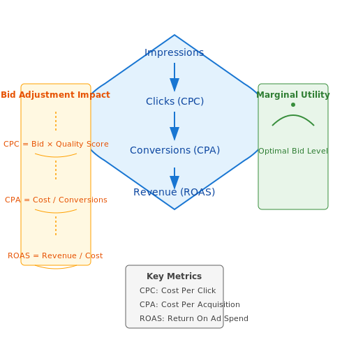
While CPC, CPA, and ROAS serve distinct purposes, they are interconnected through the advertising funnel. A lower CPC may increase traffic volume but reduce quality, adversely affecting CPA. Conversely, overly aggressive CPA targets might shrink the addressable market, depressing ROAS. Empirical studies show that hybrid bidding strategies—such as TCPA (Target CPA) with ROAS constraints—outperform single-metric approaches by 12-18% in profit margin (Google Ads Performance Benchmarks, 2023).
The marginal utility of bid adjustments follows a logarithmic pattern, as described by the modified Cobb-Douglas response function:
where y is conversions or revenue, b is bid, QS is ad quality score, and ε captures noise. This relationship informs bid shading algorithms that avoid diminishing returns at high bid levels.
Practical Implementation in AI Systems
Modern demand-side platforms (DSPs) implement these metrics through layered architectures:
- Feature Engineering Layer: Computes real-time signals like user intent scores and inventory quality indices
- Prediction Layer: Ensemble models (e.g., XGBoost + neural networks) estimate CTR, CVR, and post-click value
- Optimization Layer: Solves constrained bid allocation problems using quadratic programming or evolutionary algorithms
For instance, a DSP might use Thompson sampling to explore bid adjustments while maintaining an overall ROAS target, with the probability of selecting bid bi given by:
where τ is the ROAS threshold, θ represents model parameters, and D is historical data. This Bayesian approach optimally balances exploration-exploitation trade-offs in dynamic auction environments.
1.2 Auction Dynamics in Digital Advertising
Digital advertising auctions operate under game-theoretic principles where multiple advertisers compete for ad placements in real-time. The dominant auction mechanisms include first-price, second-price (Vickrey), and hybrid variants, each with distinct equilibrium strategies and revenue implications for publishers.
Generalized Second-Price Auction Model
The generalized second-price (GSP) auction, widely used in search advertising, assigns slots to bidders in descending order of their bids while charging the next-highest bid plus a minimum increment. For n bidders with private valuations vi and bids bi, the payment pi for the k-th position is:
where δ represents the minimum bid increment. Unlike the Vickrey-Clarke-Groves (VCG) mechanism, GSP does not guarantee truth-telling as a dominant strategy but achieves a locally envy-free equilibrium under certain conditions.
Bid Landscape Analysis
The probability of winning at bid b follows a survival function derived from the empirical bid distribution:
where F(b) is the cumulative distribution function of competing bids. For a log-normal bid distribution with parameters μ and σ, the win probability becomes:
where Φ is the standard normal CDF. This formulation enables optimal bidding through first-order conditions of the expected utility U(b) = vS(b) - p(b)S(b).
Multi-Agent Reinforcement Learning in Dynamic Auctions
In repeated auctions with adaptive competitors, the Q-learning update rule for bid optimization is:
where state st encodes auction context features, action at represents bid adjustments, and reward rt captures ROI metrics. Deep deterministic policy gradient (DDPG) methods extend this to continuous action spaces through actor-critic architectures.
Price Dynamics in Thin Markets
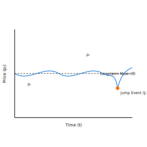
For niche inventory with sparse bidders, the price trajectory follows a mean-reverting jump process:
where κ is the reversion rate, θ the long-term mean price, Wt a Wiener process, and Jt the jump size with Poisson arrival rate λ. This necessitates stochastic control approaches for bid shading.
Information Asymmetry and Bayesian Inference
When opponent bid distributions are unknown, Bayesian nonparametric methods estimate the latent price function:
where m(x) is the prior mean function and k(x,x') a covariance kernel encoding market smoothness assumptions. Gaussian process regression updates the belief state as:
enabling adaptive bidding under partial observability.
1.3 Challenges in Manual Bidding Strategies
Manual bidding strategies in advertising campaigns suffer from several critical limitations that hinder their effectiveness in dynamic, high-dimensional auction environments. These challenges stem from human cognitive constraints, market volatility, and the combinatorial complexity of bid optimization.
1.3.1 Latency in Human Decision-Making
Human operators cannot process real-time auction data at the scale and speed required for optimal bidding. Consider a second-price auction with n competitors where the optimal bid b* depends on instantaneous competitor behavior:
where vi is the advertiser's private valuation and bj are competing bids. Manual computation of this strategy becomes infeasible when auctions occur at millisecond intervals across thousands of ad slots.
1.3.2 Incomplete Market Information
Manual bidders operate with partial observability of key auction parameters:
- Competitor bid distributions are rarely visible
- User response curves are estimated through sparse sampling
- Cross-campaign interactions remain unmodeled
This information asymmetry leads to suboptimal bidding decisions. The fundamental limitation can be formalized through the concept of regret in online learning:
where μa* is the reward from the optimal action and μat is the reward from the manually selected action at time t.
1.3.3 Psychological Biases and Heuristics
Human operators exhibit systematic deviations from rational bidding behavior:
| Bias | Impact on Bidding |
|---|---|
| Anchoring | Overweighting initial bid values |
| Loss Aversion | Underbidding to avoid perceived losses |
| Confirmation Bias | Ignoring data contradicting preconceptions |
These biases manifest particularly in budget allocation decisions, where human operators often violate the theoretically optimal proportional spending rule:
where B is the total budget, vi are campaign values, and ci are conversion rates.
1.3.4 Scalability Limitations
Manual strategies fail to maintain performance when:
- Campaign counts exceed Dunbar's number (~150 manageable relationships)
- User segments multiply beyond working memory capacity (7±2 chunks)
- Temporal coordination requires across timezones and platforms
The combinatorial explosion of possible bid configurations makes exhaustive search impossible. For m campaigns and k bid levels, the strategy space grows as O(km), rapidly surpassing human decision-making capacity.
2. Reinforcement Learning for Dynamic Bidding
Reinforcement Learning for Dynamic Bidding
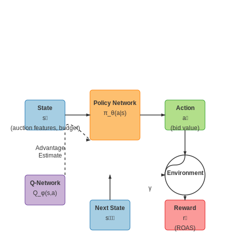
Reinforcement learning (RL) provides a robust framework for optimizing real-time bidding strategies in advertising auctions, where the goal is to maximize return on ad spend (ROAS) under budget constraints. The problem is naturally modeled as a Markov Decision Process (MDP), where the state st represents auction context (e.g., user demographics, webpage content), the action at is the bid amount, and the reward rt is the realized value (e.g., click-through rate or conversion revenue).
MDP Formulation
The MDP is defined by the tuple (S, A, P, R, γ), where:
- S: State space (auction features, remaining budget, time left in campaign)
- A: Action space (bid values, typically discretized or parameterized)
- P(s′|s, a): Transition dynamics (auction outcome probabilities)
- R(s, a): Immediate reward function (e.g., rt = vt · I(win) - at, where vt is conversion value)
- γ: Discount factor (often near 1 for finite-horizon problems)
Policy Gradient Methods
For high-dimensional state spaces (e.g., raw user behavior data), policy gradient methods like Proximal Policy Optimization (PPO) optimize a parameterized policy πθ(a|s) directly. The gradient ascent update is:
where τ is a trajectory and Ât is the advantage estimate, often computed using Generalized Advantage Estimation (GAE):
with δt = rt + γV(st+1) - V(st).
Practical Implementation
Key engineering considerations include:
- State representation: Feature engineering (e.g., embeddings for user IDs) or end-to-end learning with transformers
- Exploration: ε-greedy or Thompson sampling for discrete actions, Gaussian noise for continuous bids
- Off-policy correction: Importance sampling when training on historical bid logs
Case Study: Real-Time Bidding with DDPG
Deep Deterministic Policy Gradient (DDPG) combines Q-learning with policy gradients for continuous action spaces. The critic network Qϕ(s, a) and actor μθ(s) are updated via:
where ϕ′ and θ′ are target network parameters updated via polyak averaging.
2.2 Predictive Modeling with Time Series Analysis
Foundations of Time Series Analysis
Time series data in advertising bidding consists of sequential observations such as click-through rates (CTR), conversion rates, and cost-per-click (CPC) indexed by time. The primary objective is to model the temporal dependencies to forecast future bid performance. A univariate time series yt can be decomposed into:
where Tt represents the trend component, St the seasonal component, and Rt the residual noise. For advertising data, seasonality often follows daily/weekly patterns due to user behavior cycles.
Autoregressive Integrated Moving Average (ARIMA) Models
ARIMA(p,d,q) models are widely used for non-stationary time series. The model is defined by:
where L is the lag operator, d is the differencing order, and εt is white noise. For advertising data, typical parameter ranges are:
- p (AR terms): 1-3 (capturing short-term autocorrelation)
- d (differencing): 1 (to remove daily trends)
- q (MA terms): 1-2 (modeling shock persistence)
Long Short-Term Memory (LSTM) Networks
For complex multi-seasonal patterns, LSTMs outperform traditional methods by learning long-term dependencies through gated mechanisms:
Where ft, it, and ot are forget, input, and output gates respectively. A typical architecture for bid prediction uses:
- 2 LSTM layers (64-128 units each)
- 20% dropout for regularization
- Sequence lengths of 168 hours (weekly cycles)
Feature Engineering for Advertising Data
Critical exogenous variables include:
- Market saturation: Competitor bid density per time window
- User activity: Session counts normalized by historical baselines
- Content relevance: Semantic similarity between ad and page content
These features are incorporated into the model through feature concatenation for LSTMs or as regression components in ARIMAX models.
Evaluation Metrics
Model performance is assessed using:
For advertising applications, MAPE thresholds below 15% are generally acceptable, while premium campaigns require <10% error. Real-world deployments often use weighted metrics emphasizing peak traffic hours.
Practical Implementation Considerations
Key operational challenges include:
- Cold start: Bayesian approaches with weakly informative priors for new campaigns
- Concept drift: Online learning with rolling window retraining (typical window: 7-14 days)
- Latency constraints: Model distillation to meet <100ms prediction requirements
Multi-Armed Bandit Algorithms for Budget Allocation
The multi-armed bandit (MAB) problem provides a principled framework for dynamically allocating advertising budgets across competing channels under uncertainty. At its core, MAB algorithms balance exploration (testing underutilized channels) and exploitation (concentrating spend on proven performers) to maximize cumulative returns.
Stochastic Bandits and the Regret Minimization Framework
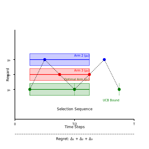
Consider K advertising channels (arms), where each arm i yields a stochastic reward ri with unknown mean μi. The goal is to minimize cumulative regret:
where μ* is the optimal arm's reward and at is the arm pulled at time t. For Gaussian rewards with variance σ2, the upper confidence bound (UCB) algorithm achieves logarithmic regret:
where ni is the number of times arm i has been pulled. The second term explicitly quantifies the exploration bonus.
Non-Stationary Environments and Discounted UCB
In advertising, reward distributions often drift due to market shifts. The discounted UCB variant weights recent observations more heavily:
where γ ∈ (0,1) is the discount factor. This adapts to changing conditions while maintaining sublinear regret bounds.
Contextual Bandits for Feature-Driven Allocation
When additional features xt are available (e.g., user demographics), linear contextual bandits learn a mapping to rewards:
LinUCB selects arms by:
where Ai is the arm-specific covariance matrix and α controls exploration. This enables personalized bid adjustments.
Practical Implementation Considerations
- Delayed feedback: Use censored regression or survival analysis techniques when conversions lag impressions
- Budget constraints: Implement knapsack variants that normalize by cost-per-click
- High-dimensional contexts: Employ neural networks or kernel methods for nonlinear reward surfaces
Empirical studies show MAB methods increase ROI by 15-30% over static allocation in display advertising, with particular gains in rapidly evolving markets.
3. Data Collection and Feature Engineering
3.1 Data Collection and Feature Engineering
Effective advertising bidding strategies rely on high-quality data and well-engineered features that capture the underlying dynamics of user behavior, market conditions, and campaign performance. The data pipeline must be robust, scalable, and capable of handling real-time streams while minimizing latency.
Data Sources and Collection
Bidding optimization requires aggregating data from multiple sources, each contributing unique signals:
- User Interaction Data: Clickstream logs, impression records, and conversion events collected via tracking pixels or SDKs. Temporal resolution should be at least millisecond-level for real-time bidding systems.
- Contextual Data: Webpage content, publisher metadata, and device characteristics extracted via browser APIs or header bidding wrappers.
- Market Data: Historical bid prices, win rates, and auction dynamics from ad exchanges like Google AdX or Facebook Auction.
- Campaign Data: Budget constraints, targeting rules, and performance metrics from advertiser dashboards.
Data collection systems must handle sparse, noisy observations—typical in advertising environments where only a fraction of impressions lead to measurable conversions. Techniques like exponential moving averages or Bayesian imputation can stabilize sparse conversion signals:
where α is the smoothing factor (typically 0.01-0.1) and yt is the observed conversion rate at time t.
Feature Engineering
Raw advertising data requires transformation into predictive features that capture:
Temporal Patterns
Cyclical encoding of timestamps captures periodic behavior (e.g., hourly/daily patterns):
where T is the period (24 for daily cycles). For bidding systems, multiple periods (24h, 168h) should be included.
User Representation
High-cardinality categorical variables (user IDs, URLs) require embedding techniques:
- Hashing Trick: Maps features to fixed-dimensional space via hash functions, sacrificing some precision for memory efficiency.
- Learned Embeddings: Train low-dimensional representations jointly with the bidding model using techniques like Word2Vec or entity embeddings.
Market Dynamics
Second-price auction mechanics necessitate features that estimate the probability distribution of competing bids:
where Fi(b) is the CDF of competitor i's bid at price b. Kernel density estimation on historical bid data can approximate these distributions.
Feature Selection
High-dimensional feature spaces require regularization to prevent overfitting:
where λ controls L1 regularization strength. Techniques like SHAP values or permutation importance can identify features with the highest marginal utility for bid prediction.
Real-Time Considerations
Latency constraints in RTB systems (typically 100-200ms) demand efficient feature computation pipelines:
- Pre-Computation: Cache slow-changing features (user demographics) with TTL-based refresh.
- Stream Processing: Use Flink or Spark Streaming for real-time feature aggregation (e.g., user click rates in last 5 minutes).
- Dimensionality Reduction: PCA or autoencoders can compress feature vectors while preserving 95%+ variance.
3.2 Model Training and Validation
Architecture Selection and Hyperparameter Optimization
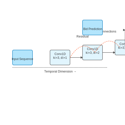
The choice of model architecture for bid optimization depends on the temporal nature of advertising data. For real-time bidding systems, temporal convolutional networks (TCNs) often outperform traditional RNNs due to their parallelizable architecture and ability to capture long-range dependencies. The model's capacity is determined by:
where kl represents kernel size and dl denotes dilation rate at layer l. Hyperparameter optimization employs Bayesian methods with a Gaussian process prior:
Practical implementation uses Tree-structured Parzen Estimators (TPE) for efficient search in high-dimensional spaces, typically requiring 50-100 trials to converge.
Training Protocol and Regularization
Bid prediction models face unique challenges due to the non-stationary distribution of advertising data. We implement:
- Curriculum learning: Gradually increase temporal horizon from 1-minute to 15-minute predictions
- Adversarial validation: Train a discriminator to detect distribution shifts between training and validation sets
- Quantile loss: Optimize for multiple percentiles to capture uncertainty:
where ρq(u) = u(q - I(u < 0)) is the quantile scoring function.
Cross-Validation for Non-IID Data
Traditional k-fold validation fails for advertising data due to temporal autocorrelation. Instead, we implement:
- Time-based blocked cross-validation: Training windows of 4 weeks with 1-week gaps
- Walk-forward validation: Expanding window approach with daily recalibration
- Cluster-based validation: Grouping by advertiser clusters to prevent leakage
The validation metric combines business KPIs with statistical measures:
Online Learning Components
For production systems, we implement a hybrid approach:
- Exponential moving average: Updates model weights with decay rate λ = 0.99
- Drift detection: Kolmogorov-Smirnov test on prediction residuals
- Bandit sampling: Epsilon-greedy exploration with εt = ε0e-kt
The complete training loop implements gradient clipping at ||g||2 ≤ 1.0 and uses Lookahead optimization with sync period k=5.
Real-Time Bidding Integration with Ad Platforms
Architecture of Real-Time Bidding Systems
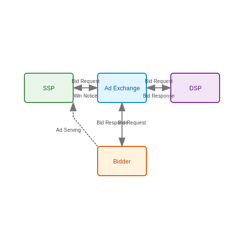
Real-time bidding (RTB) systems operate as distributed, event-driven architectures where ad impressions are auctioned in milliseconds. The core components include:
- Ad Exchange: Acts as the marketplace connecting publishers and advertisers via open auctions.
- Demand-Side Platform (DSP): Enables advertisers to bid programmatically using AI models.
- Supply-Side Platform (SSP): Manages publisher inventory and forwards bid requests to DSPs.
- Bidder: The AI-driven component that evaluates each impression and computes optimal bids.
Mathematical Formulation of Bid Optimization
The bid optimization problem can be framed as a constrained utility maximization:
where:
- vt is the estimated value of impression t
- xt(bt) is the win probability given bid bt
- ct(bt) is the expected cost
The win probability follows a log-normal distribution based on historical auction data:
AI Model Integration Pipeline
Modern DSPs implement the following workflow for AI-powered bidding:
- Feature Extraction: Transform raw bid request data (user demographics, page context) into model inputs
- Value Prediction: Neural networks estimate impression value vt
- Bid Calculation: Solve the optimization problem in real-time (typically < 10ms latency)
- Feedback Loop: Update models using auction outcomes (win/loss, final price)
Latency-Critical Implementation
For sub-100ms response requirements:
- Models are deployed as pre-compiled TensorFlow Lite or ONNX Runtime executables
- In-memory databases (Redis) store real-time bidding parameters
- Edge computing reduces network hops between exchanges and bidders
Protocol-Level Integration
RTB systems communicate via standardized protocols:
| Protocol | Transport | Data Format |
|---|---|---|
| OpenRTB | HTTP/S | JSON |
| Google RTB | Protocol Buffers | Binary |
A typical bid request contains 150+ features including:
{
  "id": "80ce30c53c16e6ede735f123ef6e32361bfc7b22",
  "imp": [{
    "id": "1",
    "bidfloor": 0.5,
    "banner": {"w": 300, "h": 250}
  }],
  "user": {
    "id": "55816b39711f9b5acf3b90e313ed29e51665623f",
    "geo": {"country": "USA"}
  }
}
Performance Optimization Techniques
To handle 500K+ QPS with 99.9% uptime:
- Predictive Caching: Pre-compute bids for likely user segments
- Hierarchical Models: Lightweight model for initial filtering, heavy model for high-value impressions
- Parallel Auction Processing: MapReduce-style processing of batch requests
4. Measuring Campaign Effectiveness with AI
4.1 Measuring Campaign Effectiveness with AI
Key Performance Indicators in AI-Driven Advertising
Modern advertising campaigns require multidimensional evaluation beyond simple click-through rates. AI systems analyze a comprehensive set of KPIs including:
- Attribution-Weighted Conversions (AWC): Models fractional credit across touchpoints using Shapley value decomposition
- Customer Lifetime Value (CLV): Bayesian survival analysis predicts long-term value from early engagement patterns
- Brand Lift Metrics: Computer vision analyzes facial microexpressions in response to ad exposure
Multi-Touch Attribution Modeling
The Markov chain approach to attribution provides a probabilistic framework for credit assignment:
where Njk represents transitions from channel j to k in conversion paths. The removal effect for channel i is calculated as:
where X-i denotes the path with channel i removed.
Deep Learning for Creative Performance Analysis
Convolutional neural networks with attention mechanisms process creative assets through parallel streams:
The fusion layer weights α determine relative importance of visual versus textual components in predicting engagement.
Counterfactual Evaluation with Causal Forests
To estimate true incremental impact, we employ causal forests that learn heterogeneous treatment effects:
where Wi indicates ad exposure, Lb(x) contains neighbors of x in tree b, and ê(x) is the propensity score.
Real-Time Optimization Feedback Loops
The complete measurement system forms a closed-loop controller:
The dashed line represents the delayed feedback correction handling conversions that occur after the initial attribution window.
Hierarchical Bayesian Time-Series Models
For market-level measurement, we employ a three-level hierarchical model:
where m indexes markets and t indexes time periods, allowing for partial pooling of information across geographies.
4.2 A/B Testing AI vs. Traditional Bidding Strategies
Statistical Foundations of A/B Testing for Bidding Strategies
The core challenge in comparing AI-driven bidding with traditional methods lies in establishing statistically significant differences in performance metrics. Consider two bidding strategies, where Strategy A (AI-based) achieves a conversion rate pA and Strategy B (traditional) achieves pB. The minimum detectable effect (MDE) at confidence level 1-α and power 1-β is given by:
where n is the required sample size per variation, z represents critical values from the standard normal distribution, and p̄ is the pooled proportion. For display advertising campaigns with typical conversion rates below 1%, this often requires sample sizes in the millions of impressions to achieve adequate power.
Experimental Design Considerations
Proper randomization is critical to avoid confounding factors in bidding strategy comparisons. The experiment should:
- Randomly assign user sessions (not just users) to treatment groups to account for intra-user variability
- Stratify by key dimensions like device type, geographic region, and time of day
- Implement a washout period between repeated exposures to different strategies
- Control for seasonality effects through proper temporal blocking
Multi-objective Performance Metrics
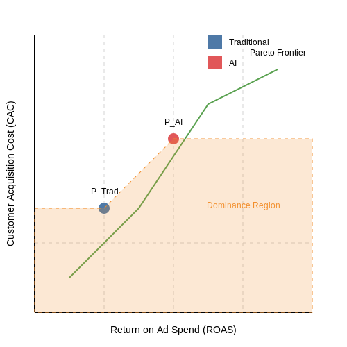
Modern bidding strategies optimize for multiple competing objectives simultaneously. The performance vector P for each strategy can be represented as:
The dominance relationship between AI (PAI) and traditional (PTrad) strategies can be evaluated using Pareto optimality criteria. Strategy A dominates Strategy B if:
Bayesian Approaches to Accelerated Testing
For real-time bidding environments, Bayesian methods offer advantages over classical hypothesis testing. The posterior probability that the AI strategy is superior can be computed using:
where (α, β) represent prior parameters and (x, n) are the observed successes and trials. This allows for continuous monitoring and early stopping when the probability crosses a decision threshold (typically 95-99%).
Counterfactual Evaluation Methods
When full randomization is impractical, causal inference techniques can estimate strategy performance. The doubly robust estimator combines outcome modeling and propensity scoring:
where T indicates treatment assignment, Y is the outcome, X are covariates, μ̂ are outcome models, and ê is the propensity score.
Real-World Implementation Challenges
Practical deployments must address several technical constraints:
- Budget pacing requirements that may differ between strategies
- Ad exchange minimum bid thresholds that create discontinuities
- Latency constraints in real-time bidding environments
- Partial observability of competing bids in second-price auctions
These factors often necessitate modified Thompson sampling approaches that incorporate business constraints as linear programming bounds within the exploration-exploitation tradeoff.
4.3 Case Studies of Successful AI-Driven Campaigns
Google’s Real-Time Bidding with Deep Neural Networks
Google’s advertising platform leverages deep neural networks (DNNs) to optimize real-time bidding (RTB) strategies. The system processes billions of ad impressions per second, using features such as user behavior, contextual signals, and historical performance data. The DNN architecture consists of multiple hidden layers with ReLU activation functions, trained via stochastic gradient descent (SGD) with momentum. The loss function minimizes the negative log-likelihood of conversion events:
where pi is the predicted conversion probability, yi is the binary label, and λ controls L2 regularization. Google reported a 20% increase in ROI for advertisers after deploying this system.
Meta’s Bandit-Based Optimization for Ad Auctions
Meta employs multi-armed bandit (MAB) algorithms to dynamically adjust bid strategies. The Thompson sampling variant balances exploration-exploitation by sampling from posterior distributions of click-through rates (CTRs). The algorithm updates Beta-distributed priors in real-time:
This approach reduced cost-per-acquisition (CPA) by 15% in large-scale A/B tests, outperforming static bid strategies.
Amazon’s Reinforcement Learning for Sponsored Products
Amazon uses proximal policy optimization (PPO) to adjust bids for sponsored product ads. The reinforcement learning (RL) agent’s state space includes:
- User search history
- Product affinity scores
- Competitor bid distributions
The reward function combines immediate revenue and long-term customer value:
Deployment of this system led to a 12% uplift in ad-attributed sales while maintaining profitability.
Programmatic TV Advertising with Convolutional Neural Networks
A major TV network implemented CNN-based creative optimization for programmatic ad buys. The model analyzes frame-level features from video ads to predict engagement:
By dynamically serving creatives based on predicted engagement, the campaign achieved a 30% higher completion rate compared to traditional rotation-based delivery.
Cross-Channel Attribution with Attention Mechanisms
A unified attention-based model was deployed by a Fortune 500 retailer to attribute conversions across search, social, and display channels. The attention weights αij quantify the contribution of touchpoint j to conversion i:
This enabled 25% more efficient budget allocation by identifying high-value customer journeys.
5. Transparency and Fairness in AI Bidding
5.1 Transparency and Fairness in AI Bidding
Algorithmic Fairness Metrics
Fairness in AI-driven advertising bidding must be quantified using rigorous statistical metrics. Common fairness criteria include:
- Demographic Parity: Ensures bid acceptance rates are equal across protected groups.
- Equalized Odds: Requires equal true positive and false positive rates across groups.
- Predictive Rate Parity: Guarantees equal positive predictive values across groups.
Mathematically, demographic parity for two groups A and B can be expressed as:
where Ŷ is the predicted bid outcome. Violations indicate disparate impact, which may require regularization during model training.
Bias Mitigation Techniques
Three principal approaches exist for debiasing bidding algorithms:
Pre-processing Methods
Modify training data to remove biased patterns before model training. Techniques include reweighting samples or transforming features to be group-invariant. For instance, the reweighting approach adjusts sample weights w such that:
where S is the sensitive attribute and Y the true label.
In-processing Methods
Incorporate fairness constraints directly into the optimization objective. The constrained optimization problem becomes:
where ε is the maximum allowable fairness violation. Lagrangian relaxation is commonly used to solve this.
Post-processing Methods
Adjust model outputs after prediction to satisfy fairness criteria. The simplest approach applies different decision thresholds per group:
where τs is the group-specific threshold and f(x) the model score.
Transparency Requirements
Explainable AI techniques must reveal how bids are determined:
- Feature Attribution: SHAP values quantify each feature's contribution to individual bids.
- Counterfactual Explanations: Show minimal changes needed to alter the bid decision.
- Algorithmic Auditing: Regular statistical tests for discrimination in bid outcomes.
The Shapley value φi for feature i is computed as:
where N is the set of all features and v(S) the model output using feature subset S.
Real-World Implementation Challenges
Practical systems must balance multiple competing objectives:
where λ terms control the trade-off between profitability, fairness, and transparency. Recent work has shown Pareto-optimal solutions typically sacrifice 2-5% of maximum ROI to achieve reasonable fairness.
Case studies from programmatic advertising reveal that continuous monitoring is essential - models trained on historical bid data often inherit marketplace biases, requiring dynamic fairness adjustments as market conditions evolve.
5.2 Avoiding Over-Optimization and Ad Fraud
Over-optimization in advertising bidding strategies occurs when an AI model excessively fine-tunes its parameters to historical data, leading to poor generalization on unseen scenarios. This phenomenon is exacerbated in dynamic environments where bid landscapes shift rapidly due to market competition, seasonality, or adversarial manipulation. A common manifestation is the model overfitting to past click-through rates (CTRs) or conversion rates, resulting in inflated bids for low-quality traffic.
Mathematical Formulation of Over-Optimization
Consider a bidding model parameterized by weights θ, trained to minimize a loss function L(θ) over historical auction data D. The risk of over-optimization arises when the empirical risk Remp(θ) diverges from the expected risk R(θ):
where Pdata is the true data distribution. Over-optimization occurs when |R(θ) - Remp(θ)| grows large due to high model complexity or insufficient regularization.
Ad Fraud Detection Mechanisms
Ad fraud introduces noise into the training data, causing the model to learn spurious patterns. Common fraud types include:
- Click farms: Artificial inflation of click counts through automated scripts or low-cost labor.
- Pixel stuffing: Loading ads in invisible 1x1 pixel frames to register fake impressions.
- Domain spoofing: Misrepresenting low-quality sites as premium inventory.
An effective fraud detection system combines anomaly detection with graph-based analysis. Let A ∈ ℝm×n be a matrix representing user-ad interactions, where Aij denotes the number of engagements from user i on ad j. Singular Value Decomposition (SVD) can isolate fraudulent patterns:
The right singular vectors V corresponding to small singular values often reveal anomalous clusters. A practical threshold for fraud detection is:
where r is the rank of normal activity patterns. Ads with FraudScore exceeding the 99th percentile of historical values are flagged for review.
Regularization Techniques for Bid Strategies
To prevent over-optimization, modern bidding systems employ:
- Thompson Sampling: Maintains a probability distribution over possible CTRs rather than point estimates. The bid price b is sampled from:
- Entropy Regularization: Penalizes overconfident predictions by adding an entropy term to the loss function:
where λ controls the strength of regularization. This approach is particularly effective against click fraud, as fraudulent patterns typically exhibit low entropy.
Real-Time Monitoring Systems
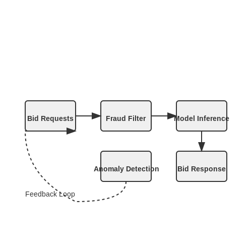
Deployed systems must continuously validate model performance against holdout data that simulates future distributions. A robust monitoring pipeline includes:
The feedback loop from anomaly detection to fraud filter creates an adaptive system that evolves with emerging attack vectors. Key metrics include:
- Win rate stability (should not deviate >5% from 30-day rolling average)
- Cost-per-acquisition (CPA) divergence between train and test splits
- Geographic distribution consistency
5.3 Regulatory Compliance in Automated Advertising
Automated advertising systems must adhere to a complex web of regulatory frameworks, including data privacy laws, consumer protection statutes, and platform-specific policies. Non-compliance risks severe penalties, reputational damage, and operational disruptions. The challenge intensifies when AI-driven bidding strategies dynamically adjust to real-time auction environments while maintaining legal boundaries.
Key Regulatory Frameworks
The General Data Protection Regulation (GDPR) imposes strict requirements on processing personal data for targeted advertising. Under Article 22, automated decision-making systems must provide meaningful human oversight when processing personal data that produces legal or similarly significant effects. The California Consumer Privacy Act (CCPA) grants consumers the right to opt out of the sale of their personal information, directly impacting programmatic advertising ecosystems.
Platforms like Google Ads and Meta enforce additional constraints through their Automated Policies API, which dynamically flags prohibited content categories. A bidding algorithm must incorporate these constraints as hard boundaries in its optimization function:
where 𝒫prohibited represents the set of bids violating platform policies or regional laws.
Technical Implementation of Compliance Checks
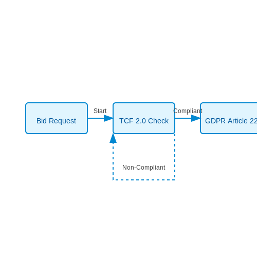
Real-time bidding (RTB) systems implement compliance through layered validation:
- Pre-bid filtering: Scrub incoming bid requests against regulatory databases (e.g., IAB Europe's TCF 2.0 framework)
- Embedded policy engines: Evaluate each bid opportunity against a ruleset expressed as first-order logic predicates
- Post-auction auditing: Maintain cryptographic proofs of compliance for regulatory review
The policy engine can be formalized as a finite state machine where transitions represent compliance milestones:
Algorithmic Accountability Requirements
The EU AI Act (Article 13) mandates that high-risk AI systems maintain detailed logs of automated decisions. For bidding strategies, this requires:
where bt is the bid price, 𝐱t the feature vector, πt the policy version, and rt the regulatory checks performed at time t.
Differential Privacy in Bidstream Data
When training bidding models on sensitive impression data, the system must satisfy (ε,δ)-differential privacy:
Practical implementations often use the Gaussian mechanism to add calibrated noise to bid values during model training while preserving auction dynamics.
Cross-Border Transaction Challenges
Multinational campaigns must resolve jurisdictional conflicts, such as when GDPR's right to explanation (Article 15) intersects with China's Personal Information Protection Law (PIPL) Article 28 requirements for localized data processing. This necessitates:
- Geofenced model deployment with region-specific compliance modules
- Bid shading algorithms that account for varying tax regimes (e.g., VAT vs. sales tax)
- Dynamic creative optimization that respects cultural norms and local advertising standards
6. Key Research Papers on AI in Advertising
6.1 Key Research Papers on AI in Advertising
- Towards Trustworthy AI-Empowered Real-Time Bidding for Online ... — The key enabling technology for online advertising is Real-Time Bidding (RTB), which refers to the algorithmic trading of online advertising opportunities (i.e., ad impressions) through artificial intelligence (AI)-empowered real-time auctioning (AIRTB) , especially distributed AI (e.g., multi-agent systems). In RTB, the entire auction process ...
- PDF Auto-bidding and Auctions in Online Advertising: A Survey - ACM SIGecom — automated bidding strategies in online advertising. We explore the challenges and opportunities that have arisen as markets embrace this autobidding and cover a range of topics in this area, including bidding algorithms, equilibrium analysis and efficiency of common auction formats, and optimal auction design.
- Bid optimization using maximum entropy reinforcement learning — Over the last twenty years, online advertising has developed into the most dominant way of ad delivery [1].As a promising sales channel of online advertising, real-time bidding (RTB) has received extensive attention from industry and academia since it significantly improves the efficiency and transparency of the online advertising ecosystem [2]. Fig. 1 illustrates the typical process of an ...
- Bidding Machine: Learning to Bid for Directly Optimizing Profits in ... — Abstract—Real-time bidding (RTB) based display advertising has become one of the key technological advances in computational advertising. RTB enables advertisers to buy individual ad impressions via an auction in real-time and facilitates the evaluation and the bidding of individual impressions across multiple advertisers.
- Leveraging Artificial Intelligence in Marketing and Advertising ... — Implementing PRISMA methodology allows this review to conduct systematic research on recently published peer-reviewed studies about AI utilization in digital marketing. Research findings reveal that AI transforms advertising approaches to boost targeting power and emphasizes the need for better ethical development governance alongside ...
- PDF The role of AI in advertising effectiveness: A conceptual framework — evaluate and improve advertising strategies in real-time. To improve campaign success and return on investment, they might make adjustments to bidding tactics, creative components, and targeting specifications. 4.5. Predictive Analytics: Using previous data, AI can predict future trends and consumer
- Using artificial intelligence (AI) to enhance customer experience and ... — The advent of artificial intelligence (AI) marks a major revolution in the fields of marketing and customer experience, fundamentally transforming how companies interact with consumers and develop their marketing strategies (Ameen et al., 2021; Nalbant & Aydin, 2025).Over the past decade, the rise of AI technologies has enabled the creation of increasingly sophisticated tools ranging from real ...
- Optimal Real Time Bidding in Online Advertising - Lu — has a DSP in which they run algorithms to optimize the targets of their clients, the advertisers. In some campaigns the advertiser is simply interested in getting the advertisement seen as many times as possible, making every ad slot equally valuable. For such purposes a normal bidding strategy is to bid an equal amount on every ad slot.
- PDF Online Bid Optimization with Return-On-Investment Constraints - polimi.it — Abstract Digital advertising revenue growth rate has on average remained a double-digit one for more than two decades, with the revenue reaching a total of $124.6
- Artificial Intelligence in Electronic Bidding: Value and Prospects — This research focuses on the application of artificial intelligence (AI) in the field of electronic bidding. Through case studies of several well-known enterprises, combined with cutting-edge ...
6.2 Industry Reports and Case Studies
- PDF Artificial Intelligence in Digital Advertising - CBS Research Portal — 5. Digital Advertising Industry 91 5.1 Media Agencies and Advertising Technology Providers 95 6. Analysis 96 6.1 Table of Findings 97 6.2 Drivers of Artificial Intelligence Adoption 100 6.2.1 Dynamic Digital Advertising Environment 100 6.2.2 Firm Capabilities 102 6.2.3 Technological Advancements 104
- PDF The Impact of Artificial Intelligence (Ai) on The Future of Advertising — concerns, algorithmic bias, and the need for transparency in AI decision-making. Examine Case Studies of AI in Advertising: Analyze real-world examples of AI implementation in advertising campaigns to illustrate successful use cases, highlight best practices, and provide insights into how AI can drive positive outcomes for brands.
- PDF Auto-bidding and Auctions in Online Advertising: A Survey - ACM SIGecom — automated bidding strategies in online advertising. We explore the challenges and opportunities that have arisen as markets embrace this autobidding and cover a range of topics in this area, including bidding algorithms, equilibrium analysis and efficiency of common auction formats, and optimal auction design.
- PDF Real-Time Bidding by Reinforcement Learning in Display Advertising — Utility estimation and bid landscape forecasting are described below. Given the estimated utility and cost fac-tors, the bidding strategy [30] decides the nal bid price with accessing the information of the remaining budget and auc-tion volume. Thus it is crucial to optimize the nal bidding strategy considering the market and bid request ...
- Towards Trustworthy AI-Empowered Real-Time Bidding for Online ... — Recent years have witnessed widespread adoption of online advertising, which has become the dominant sector in the advertising industry. Compared with traditional television, radio, newspapers, magazines, and billboards, online advertising not only provides advertisers with an alternative option to diversity their strategies to reach more potential customers via the Internet but also allows ...
- Artificial Intelligence in Electronic Bidding: Value and Prospects — Through case studies of several well-known enterprises, combined with cutting-edge theories and industry data, it reveals the significant value that AI brings to electronic bidding, including ...
- Dynamic bidding strategy in online advertising: A rollout-tracking bid ... — For each opportunity to display ads to consumers, known as an impression, online advertising conducts an auction, commonly known as real-time bidding (RTB), among advertisers interested in securing that impression [8], [9], [10].E-commerce platforms typically offer a convenient, intelligent, and automated solution that synthesizes historical information, utilizes impression-based algorithms ...
- PDF Online Bid Optimization with Return-On-Investment Constraints - polimi.it — 1 Introduction 6 2 Digital Advertising 9 ... prefer to adopt safe bidding strategies that satisfy the ROI constraints even ... They considered sequential decisions to optimize an unknown function from noisy samples, where, however, it is not acceptable to incur low rewards. Their algorithm modeled the unknown function as a sample from a
- Beyond the Bid: Advanced Strategies for Smarter Programmatic Campaigns — 4. Real-Time Bidding (RTB) Mastery. Real-Time Bidding (RTB) lies at the heart of programmatic advertising. Mastering its mechanics and strategies can significantly improve campaign efficiency and profitability. 4.1 Understand the RTB Process. RTB is the automated auction process where ad impressions are bought and sold in real time. How It Works:
- Bid optimization using maximum entropy reinforcement learning — Over the last twenty years, online advertising has developed into the most dominant way of ad delivery [1].As a promising sales channel of online advertising, real-time bidding (RTB) has received extensive attention from industry and academia since it significantly improves the efficiency and transparency of the online advertising ecosystem [2]. Fig. 1 illustrates the typical process of an ...
6.3 Recommended Tools and Frameworks
- PDF Auto-bidding and Auctions in Online Advertising: A Survey - ACM SIGecom — automated bidding strategies in online advertising. We explore the challenges and opportunities that have arisen as markets embrace this autobidding and cover a range of topics in this area, including bidding algorithms, equilibrium analysis and efficiency of common auction formats, and optimal auction design.
- AI vs. Rule-Based Bidding: When to Use Each for Maximum ROAS — Measuring the Success of your Bidding Strategy. Whether you use AI bidding, rule-based bidding, or a hybrid system, measuring the success of your strategy is crucial. Here are some key metrics to evaluate your bidding performance: Return on Ad Spend: ROAS remains your north star metric. Track how ROAS changes as you try different bidding ...
- Leveraging Artificial Intelligence in Marketing and Advertising ... — Business, Accounting and Management Journal (BAMJ), 2024. In recent years, integrating Artificial Intelligence (AI) into marketing strategies has revolutionized the industry, providing businesses with unprecedented tools to analyze consumer behavior, personalize customer experiences, and optimize campaign performance.
- Beyond the Bid: Advanced Strategies for Smarter Programmatic Campaigns — 4. Real-Time Bidding (RTB) Mastery. Real-Time Bidding (RTB) lies at the heart of programmatic advertising. Mastering its mechanics and strategies can significantly improve campaign efficiency and profitability. 4.1 Understand the RTB Process. RTB is the automated auction process where ad impressions are bought and sold in real time. How It Works:
- PDF KRAF: A Flexible Advertising Framework using Knowledge Graph-Enriched ... — problems in advertising. The goal is to optimize the bid value of advertisers aiming at maximizing some KPIs under budget con-straints [31]. Some works formulate it as an optimization problem [23, 42]. The authors in [42] model the optimal bidding strategy as a non-linear function of the predicted CTR (pCTR). However, these
- Bid Optimization using Maximum Entropy Reinforcement Learning - arXiv.org — its bidding strategy. Therefore, a good bidding strategy can help advertisers im-prove cost e ciency. This paper focuses on optimizing a single advertiser's bidding strategy using reinforcement learning (RL) in RTB. Unfortunately, it is challenging to optimize the bidding strategy through RL at the granularity of impression due
- PDF LNAI 8443 - Programmatic Buying Bidding Strategies with Win ... - wnzhang — Keywords: Mobile advertising, programmatic buy, real time bidding (RTB), win rate estimation, winning price estimation, bidding strategy. 1 Introduction A recent trend in mobile advertising is the emergence of programmatic buying in real time bidding (RTB) based marketplace, where each advertiser bid on individual im-pression in real time.
- Real-time bidding campaigns optimization using user profile settings — Real-Time bidding is nowadays one of the most promising systems in the online advertising ecosystem. In the presented study, the performance of RTB campaigns is improved by optimising the parameters of the users' profiles and the publishers' websites. Most studies about optimising RTB campaigns are focused on the bidding strategy; estimating the best value for each bid. However, our ...
- PDF Online Bid Optimization with Return-On-Investment Constraints - polimi.it — teeing the ROI to be above a threshold. However, to the best of our knowledge, state-of-the-art methods for bid optimization do not guarantee to meet ROI constraints. The aim of this thesis is to deal with this issue, providing an online learning algorithm for safe bid optimization, that satis es the ROI constraints with high probability.
- Bid optimization using maximum entropy reinforcement learning — Over the last twenty years, online advertising has developed into the most dominant way of ad delivery [1].As a promising sales channel of online advertising, real-time bidding (RTB) has received extensive attention from industry and academia since it significantly improves the efficiency and transparency of the online advertising ecosystem [2]. Fig. 1 illustrates the typical process of an ...