Training AI on Public Transit Ridership Data
1. Key Data Sources and Collection Methods
Key Data Sources and Collection Methods
Automated Fare Collection (AFC) Systems
AFC systems, such as contactless smart cards (e.g., Oyster, ORCA, or Clipper), generate granular ridership data at the individual trip level. Each transaction record typically includes:
- Card identifier (anonymized)
- Timestamp of boarding and alighting
- Location (station ID or GPS coordinates)
- Fare calculation metadata
The temporal resolution of AFC data enables modeling demand fluctuations at minute-level precision. Spatial resolution depends on the sensor density, with metro systems typically offering station-level accuracy while buses provide route-segment granularity through GPS pings.
Automatic Passenger Counting (APC) Systems
APC systems use infrared sensors, weight sensors, or computer vision to count boarding and alighting passengers per vehicle. Modern implementations achieve 95-98% accuracy through multi-modal sensor fusion:
Time-stamped APC data streams integrate with vehicle telemetry (GPS, accelerometer) to create spatiotemporal occupancy matrices. The resulting 4D tensor (route × time × direction × load factor) serves as input for convolutional LSTM networks predicting crowding.
General Transit Feed Specification (GTFS)
The GTFS standard provides static schedule data in a relational format comprising:
- routes.txt: Transit line definitions
- trips.txt: Vehicle journey instances
- stop_times.txt: Timetables with dwell time distributions
When combined with real-time GTFS-RT feeds, these datasets enable hybrid models that blend scheduled operations with actual vehicle movements. The differential between planned and observed headways serves as a key feature in delay propagation models.
Mobile Network Data
Anonymized cellular signaling data from mobile operators offers metropolitan-scale origin-destination matrices. The spatial precision depends on cell tower density:
where c is signal propagation speed and τ is timing advance precision. While lacking trip purpose context, these datasets provide ground truth for validating synthetic population mobility models.
Computer Vision Systems
Onboard cameras with real-time object detection (YOLOv7, DETR) generate passenger flow analytics. Modern implementations use depth sensing to overcome occlusion challenges:
where vi is the optical flow vector and n̂ is the door normal vector. Edge computing devices process these streams locally to preserve privacy.
Data Fusion Challenges
Integrating these heterogeneous sources requires solving the correspondence problem across mismatched spatiotemporal references. The alignment process minimizes the Wasserstein distance between empirical distributions:
where Γ(μ,ν) contains all joint distributions with marginals μ (AFC data) and ν (APC data). Successful fusion enables multi-view learning architectures that outperform single-source models by 12-18% in demand prediction tasks.

1.2 Common Data Formats and Structures
Tabular Data (CSV, Parquet, SQL)
Public transit ridership data is most commonly stored in tabular formats, where each row represents an observation (e.g., a trip) and each column represents a feature (e.g., timestamp, origin, destination, fare). CSV remains widely used due to its simplicity, but columnar formats like Parquet offer superior compression and query performance for large datasets. SQL databases provide transactional integrity and support complex joins, but require schema enforcement.
For time-series heavy transit data, Parquet achieves compression ratios of 4:1 to 10:1 by leveraging dictionary encoding and run-length encoding on repeated values (e.g., station IDs).
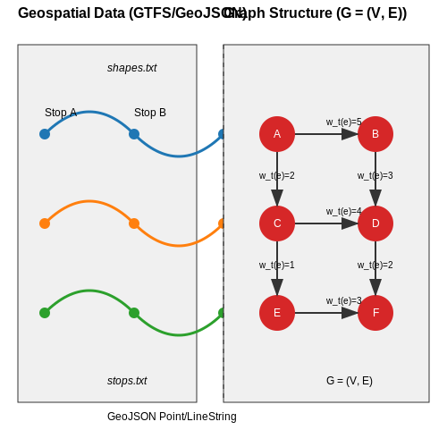
Geospatial Data (GTFS, GeoJSON, Shapefiles)
The General Transit Feed Specification (GTFS) is the de facto standard for representing transit networks, containing:
- stops.txt: Latitude/longitude of stations
- trips.txt: Vehicle trajectories with timepoints
- shapes.txt: Precise route geometries as linestrings
GeoJSON extends JSON with geometry primitives (Point, LineString, Polygon), while Shapefiles bundle multiple files (.shp, .shx, .dbf) with topological relationships. For large-scale analysis, geospatial data is often stored in PostGIS-enabled databases with R-tree indexing:
Graph Structures (NetworkX, Neo4j)
Transit networks are naturally represented as graphs G = (V, E), where vertices V are stations and edges E are connections weighted by travel time or frequency. Property graphs in Neo4j enable:
MATCH (a:Station)-[r:CONNECTS_TO]->(b:Station)
WHERE r.avg_delay > 300
RETURN a.name, b.name, r.line_id
For temporal graphs, edges gain dynamic weights wt(e) representing time-dependent congestion.
Time Series Formats (HDF5, InfluxDB)
Ridership time series require high-frequency timestamp handling. HDF5 supports chunked storage for efficient windowed queries:
Specialized TSDBs like InfluxDB optimize for time-range predicates and downsampling, critical for analyzing peak/off-peak patterns.
Unstructured Data (APC, AVL Logs)
Automated Passenger Counting (APC) and Automatic Vehicle Location (AVL) systems generate semi-structured logs with irregular schemas. These require schema-on-read approaches like:
df = spark.read.json(
   "s3://transit-logs/raw/",
   schema=StructType([
      StructField("vehicle_id", StringType()),
      StructField("events", ArrayType(MapType(StringType(), StringType())))
   ])
)
Nested structures preserve the raw fidelity needed for anomaly detection in irregular event streams.
1.3 Challenges in Data Quality and Completeness
Public transit ridership data presents unique challenges for AI training due to inherent quality and completeness issues. These challenges stem from the complex nature of urban mobility systems, where data collection mechanisms must contend with dynamic passenger flows, heterogeneous sensor networks, and operational constraints.
Missing Data Patterns
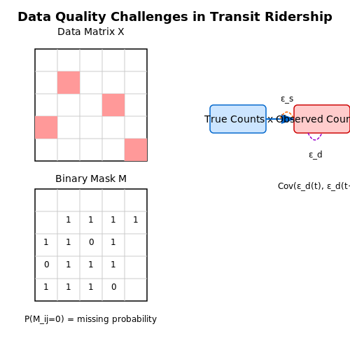
Transit systems exhibit systematic missing data patterns that violate the missing-at-random (MAR) assumption. Let X represent the complete data matrix where rows correspond to time intervals and columns represent stations. The observed data follows:
where M is a binary mask matrix and ⊙ denotes element-wise multiplication. The missingness mechanism in transit data often follows:
where ti is the time interval, sj is the station, and θ represents system-specific parameters. This spatiotemporal dependence complicates imputation as standard techniques like mean substitution or matrix factorization perform poorly when missingness correlates with latent variables.
Sensor Noise and Systematic Errors
Automated passenger counting (APC) systems introduce measurement errors that propagate through AI models. The observed count y relates to the true count x through:
where εs represents sensor-specific bias (e.g., infrared vs. pressure mat systems) and εd captures dynamic errors from environmental factors like crowding or door obstruction. These errors exhibit temporal autocorrelation:
with ρ typically ranging 0.3-0.7 for urban transit systems, invalidating the independent noise assumption in many machine learning models.
Data Fusion Challenges
Modern transit networks combine data from fare collection systems, APC sensors, and manual tallies, each with different:
- Temporal resolutions: Smart card taps (seconds) vs. APC (minutes) vs. manual counts (hours)
- Spatial coverage: Fare gates cover entry/exit points while APC sensors monitor specific vehicles
- Measurement definitions: Boardings vs. alightings vs. passenger-miles
The fusion problem requires solving a high-dimensional alignment task. For n data sources, the joint likelihood becomes:
where τi represents the unknown alignment parameters for source i. The resulting optimization is non-convex and sensitive to initialization.
Ground Truth Limitations
Validation of ridership models suffers from circular referencing - manual counts used for validation often derive from the same imperfect sensors being evaluated. The effective degrees of freedom in validation shrink dramatically when accounting for autocorrelation:
For typical ρ = 0.6 and N = 100 samples, Neff ≈ 25, severely reducing statistical power to detect model errors.
2. Handling Missing and Noisy Data
2.1 Handling Missing and Noisy Data
Public transit ridership datasets often suffer from missing entries and measurement noise due to sensor malfunctions, transmission errors, or inconsistent data collection protocols. Addressing these issues requires a combination of statistical imputation, robust estimation techniques, and domain-aware data cleaning.
Missing Data Mechanisms
Missing data in transit systems typically falls into one of three categories:
- Missing Completely at Random (MCAR): Absence bears no relation to observed or unobserved variables (e.g., random sensor failures).
- Missing at Random (MAR): Missingness depends on observed variables (e.g., ticket validators failing during peak hours).
- Missing Not at Random (MNAR): Missingness relates to unobserved factors (e.g., passengers avoiding fare gates during inspections).
For MCAR and MAR scenarios, maximum likelihood estimation provides theoretically sound imputation. The likelihood function for incomplete data decomposes as:
Advanced Imputation Techniques
Multiple Imputation by Chained Equations (MICE) outperforms single imputation for MAR data. Each incomplete variable is modeled conditional on others:
where t indexes iteration rounds and fj is a generalized linear model. For transit data, incorporate:
- Temporal autoregressive terms for time-series gaps
- Spatial correlation kernels for station-level data
- Ridership periodicity components (daily/weekly cycles)
Noise Robustness in Ridership Signals
Anomalous counts arise from fare evasion, double-counting, or equipment drift. Median Absolute Deviation (MAD) provides robust scaling:
where X̃ is the sample median. For non-stationary flows, apply wavelet shrinkage:
with threshold function δT and wavelet coefficients dj,k. The universal threshold T = σ√(2logN) works well for Gaussian noise.
Practical Implementation
For Python implementations, use:
import numpy as np
from sklearn.experimental import enable_iterative_imputer
from sklearn.impute import IterativeImputer

# MICE imputation with BayesianRidge
imputer = IterativeImputer(
    estimator=BayesianRidge(),
    n_nearest_features=5,
    initial_strategy='median',
    max_iter=20,
    tol=1e-3
)
imputed_data = imputer.fit_transform(ridership_matrix)
For real-time applications, Kalman filters with outlier rejection provide streaming imputation:
where the innovation term (zk - Hkx̂k|k-1) undergoes Huber-style robust weighting.
Temporal and Spatial Feature Extraction
Time-Series Decomposition for Ridership Patterns
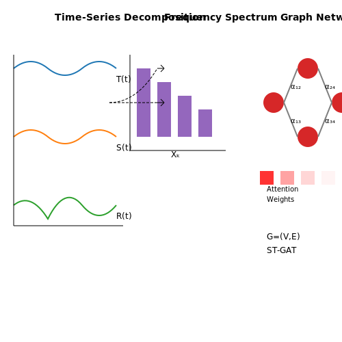
Public transit ridership data exhibits strong temporal dependencies, necessitating decomposition into trend, seasonality, and residual components. For a given ridership time series y(t), the classical additive decomposition is:
where T(t) represents long-term trends, S(t) captures periodic patterns (daily/weekly cycles), and R(t) contains irregular fluctuations. The STL (Seasonal-Trend decomposition using Loess) algorithm provides robust estimation of these components, particularly for data with multiple seasonal periods.
Fourier Transform for Periodic Feature Extraction
Discrete Fourier Transform (DFT) converts temporal patterns into frequency-domain representations, identifying dominant periodicities in ridership data. For N observations, the DFT coefficients are computed as:
Power spectral density analysis of these coefficients reveals significant frequencies corresponding to daily, weekly, and annual ridership cycles. This enables feature engineering of harmonic components that improve model performance.
Spatial Feature Engineering with Graph Networks
Transit networks naturally form graphs G = (V,E), where stations are nodes V and routes are edges E. Graph convolutional networks (GCNs) extract spatial features by aggregating information from neighboring nodes:
where à = A + I is the adjacency matrix with self-connections, D̃ is the degree matrix, and W contains learnable parameters. This captures ridership spillover effects between connected stations.
Geospatial Embeddings
Station locations can be encoded using:
- Latitude/longitude coordinates projected using Mercator or UTM systems
- Hexagonal binning for density-aware spatial aggregation
- H3 geospatial indexing for multi-resolution analysis
Spatio-Temporal Graph Attention Networks
Combining temporal and spatial features, ST-GAT models compute dynamic attention weights between nodes:
where a is a learnable attention vector and W transforms node features h. This allows the model to focus on relevant spatial relationships that vary over time.
Practical Implementation Considerations
When implementing these techniques:
- Align temporal and spatial sampling frequencies to prevent information leakage
- Normalize features across different transit modes (bus, metro, etc.)
- Handle missing data using spatial interpolation or matrix completion
- Optimize computational efficiency through hierarchical sampling in large networks
2.3 Normalization and Scaling Techniques
Public transit ridership datasets often exhibit heterogeneous scales across features—passenger counts may range in the thousands, while temperature or time-of-day indicators occupy smaller numerical ranges. Unscaled features can distort distance-based algorithms like k-nearest neighbors (k-NN) or gradient-descent optimizers in neural networks, causing convergence issues or biased feature importance. Proper normalization ensures numerical stability and equitable feature contribution.
Min-Max Normalization
Min-max scaling linearly transforms features to a fixed range, typically [0, 1]. For a feature vector X with observed values xi:
This method preserves the original distribution while compressing the dynamic range. However, it is sensitive to outliers—extreme values in ridership data (e.g., a holiday surge) can squeeze the majority of data points into a narrow interval.
Z-Score Standardization
Standardization rescales data to have zero mean and unit variance, making it suitable for algorithms assuming Gaussian distributions (e.g., linear regression, SVMs). The transformation is defined as:
where μ and σ are the mean and standard deviation of X. Unlike min-max, standardization handles outliers more gracefully but does not bound values to a specific range.
Robust Scaling
For datasets with significant outliers—common in transit data due to events or disruptions—robust scaling uses median and interquartile range (IQR):
This method is resilient to extreme values but may distort the feature distribution if the IQR is narrow.
Practical Considerations for Transit Data
- Temporal Features: Cyclic variables like hour-of-day require special treatment. Linear scaling misrepresents the circular relationship between 23:00 and 00:00. Instead, encode them as (sin(θ), cos(θ)) where θ = 2πh/24.
- Sparse Counts: Features like hourly boardings at low-ridership stations benefit from log transformation (log(1 + x)) before scaling to mitigate skew.
- Geospatial Data: Latitude/longitude coordinates should be scaled independently or projected into a local coordinate system to preserve relative distances.
Algorithm-Specific Recommendations
Tree-based models (e.g., Random Forests) are scale-invariant, but neural networks and distance-based methods require careful normalization:
- Neural Networks: Standardization (z-score) is preferred for activation function stability, especially with ReLU variants.
- k-NN/PCA: Min-max scaling ensures equal feature weighting in distance metrics like Euclidean or Manhattan.
- SVMs: Scale all features to [−1, 1] to prevent dominance by high-magnitude features.
Empirical validation is critical: use metrics like silhouette score (clustering) or reconstruction error (autoencoders) to evaluate scaling efficacy for the specific task.
3. Regression Models for Ridership Prediction
3.1 Regression Models for Ridership Prediction
Linear Regression for Baseline Ridership Forecasting
Linear regression serves as the foundational model for ridership prediction due to its interpretability and computational efficiency. Given a feature vector x containing variables like time of day, weather conditions, and historical ridership, the model predicts ridership y as:
where β0 is the intercept, βi are coefficients, and ε represents Gaussian noise. The ordinary least squares (OLS) estimator minimizes the sum of squared residuals:
For transit data, temporal autocorrelation often violates OLS assumptions. Generalized Least Squares (GLS) with an AR(1) covariance structure improves performance:
Nonlinear and Tree-Based Approaches
When ridership patterns exhibit nonlinear relationships (e.g., saturation effects during peak hours), Random Forests and Gradient Boosted Trees (GBTs) outperform linear models. A GBT with K trees predicts:
where fk are regression trees and ℱ is the space of possible trees. The XGBoost implementation uses second-order Taylor expansion for loss optimization:
with gi and hi as first/second-order gradient statistics on the loss function.
Neural Network Architectures
For high-frequency smart card data, Long Short-Term Memory (LSTM) networks capture complex temporal dynamics. The cell state update incorporates forget (ft), input (it), and output (ot) gates:
Bidirectional LSTMs process sequences both forward and backward, while attention mechanisms weight relevant historical observations:
Evaluation Metrics and Practical Considerations
Model performance is assessed using:
- Mean Absolute Percentage Error (MAPE): $$ \text{MAPE} = \frac{100\%}{n} \sum_{t=1}^n \left| \frac{y_t - \hat{y}_t}{y_t} \right| $$
- Root Mean Squared Log Error (RMSLE): Penalizes under-prediction more heavily for imbalanced ridership distributions
Feature engineering critically impacts performance. Spatial features (e.g., distance to landmarks) should be encoded via hexagonal binning (H3) to avoid coordinate system distortions. Temporal features require Fourier transforms for periodic decomposition:
where τ is the period (e.g., 24 hours for daily cycles).
3.2 Time Series Forecasting with LSTM and ARIMA
Long Short-Term Memory (LSTM) Networks
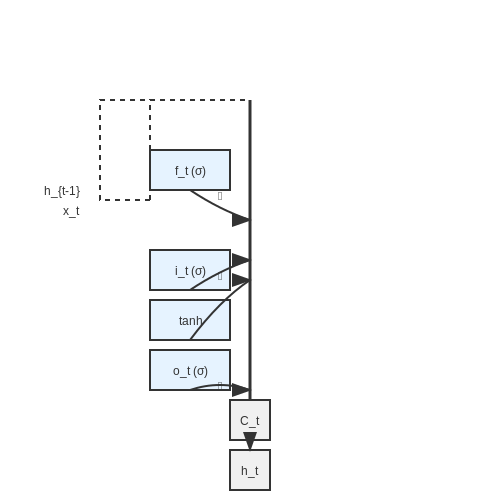
LSTMs are a specialized form of recurrent neural networks (RNNs) designed to capture long-term dependencies in sequential data. Unlike traditional RNNs, LSTMs mitigate the vanishing gradient problem through gating mechanisms. The core of an LSTM cell consists of three gates: the input gate, forget gate, and output gate, each regulated by sigmoid activations and pointwise operations.
Here, \(f_t\), \(i_t\), and \(o_t\) represent the forget, input, and output gates, respectively. \(C_t\) is the cell state, and \(h_t\) is the hidden state. The Hadamard product (\(\odot\)) denotes element-wise multiplication.
Practical Implementation for Transit Ridership
When modeling public transit ridership, LSTMs excel at capturing periodic trends (daily, weekly, or seasonal fluctuations) and irregular events (holidays, disruptions). A typical architecture includes:
- An input layer with sequence length matching the historical window (e.g., 30 days).
- One or more LSTM layers with dropout regularization.
- A dense output layer with linear activation for regression.
from tensorflow.keras.models import Sequential
from tensorflow.keras.layers import LSTM, Dense, Dropout

model = Sequential([
   LSTM(64, return_sequences=True, input_shape=(30, 1)),
   Dropout(0.2),
   LSTM(32),
   Dense(1)
])
model.compile(optimizer='adam', loss='mse')
Autoregressive Integrated Moving Average (ARIMA)
ARIMA models are a classical approach for time series forecasting, combining autoregression (AR), differencing (I), and moving averages (MA). The model is parameterized as ARIMA\((p, d, q)\):
- \(p\): Order of the autoregressive component.
- \(d\): Degree of differencing to achieve stationarity.
- \(q\): Order of the moving average component.
where \(\Delta^d\) denotes the \(d\)-th difference, \(\phi_i\) and \(\theta_j\) are coefficients, and \(\epsilon_t\) is white noise. For transit data, seasonal ARIMA (SARIMA) extensions are often necessary to account for weekly or monthly patterns.
Model Selection and Diagnostics
Key steps in ARIMA modeling include:
- Stationarity testing: Augmented Dickey-Fuller (ADF) test to determine \(d\).
- ACF/PACF analysis: Identify \(p\) and \(q\) from autocorrelation plots.
- Parameter optimization: Minimize AIC or BIC criteria via grid search.
from statsmodels.tsa.arima.model import ARIMA
from statsmodels.tsa.stattools import adfuller

# Check stationarity
result = adfuller(ridership_data)
d = 0 if result[1] < 0.05 else 1

# Fit ARIMA(1,1,1)
model = ARIMA(ridership_data, order=(1, d, 1))
results = model.fit()
Hybrid Approaches
Combining LSTM and ARIMA leverages the strengths of both methods. A common strategy is to use ARIMA for linear trend decomposition and LSTM for modeling residuals. The workflow involves:
- Fit ARIMA to the ridership data and extract residuals.
- Train an LSTM on the residuals to capture nonlinear patterns.
- Combine predictions from both models additively.
Empirical studies on transit datasets show hybrid models reduce mean absolute error (MAE) by 15–20% compared to standalone methods.
3.3 Clustering for Demand Pattern Analysis
Clustering techniques are indispensable for uncovering latent demand patterns in public transit ridership data. Unlike supervised learning, clustering operates without predefined labels, making it ideal for exploratory analysis where ridership behaviors are not yet categorized. The primary objective is to partition the dataset into homogeneous groups where intra-cluster similarity is maximized and inter-cluster dissimilarity is minimized.
Distance Metrics for Temporal-Spatial Data
Public transit data often combines temporal and spatial dimensions, necessitating specialized distance metrics. The Mahalanobis distance accounts for covariance between features, making it suitable for correlated ridership variables:
where 𝐒 is the covariance matrix of the dataset. For time-series data, Dynamic Time Warping (DTW) handles phase shifts in demand patterns:
where π represents an alignment path between sequences X and Y.
Density-Based Spatial Clustering (DBSCAN) for Anomaly Detection
DBSCAN identifies clusters as high-density regions separated by low-density areas, making it robust to noise in ridership data. Given a neighborhood radius ε and minimum points minPts, a point p is a core point if:
where N_ε(p) denotes the ε-neighborhood of p. Border points have fewer neighbors but are reachable from core points, while noise points remain unassigned. This property makes DBSCAN particularly effective for detecting irregular demand patterns caused by events or disruptions.
Gaussian Mixture Models for Probabilistic Clustering
When demand patterns exhibit overlapping distributions, Gaussian Mixture Models (GMMs) provide a probabilistic framework. The likelihood of a ridership observation 𝐱 is:
where π_k are mixture weights and μ_k, Σ_k are the mean and covariance of the k-th component. The Expectation-Maximization (EM) algorithm iteratively optimizes these parameters:
- E-step: Compute posterior probabilities γ(z_nk) for latent variables
- M-step: Update parameters using current responsibilities
Cluster Validation Indices
Quantifying cluster quality requires metrics beyond simple inertia. The Silhouette Coefficient for a sample i is:
where a(i) is the average intra-cluster distance and b(i) is the smallest inter-cluster distance. For density-based clusters, the Davies-Bouldin Index compares scatter within clusters to separation between them:
where σ_i is the average distance from points in cluster i to its centroid c_i.
Multi-View Clustering for Heterogeneous Data
Transit data often comes from disparate sources (e.g., fare collection, GPS, weather). Multi-view clustering integrates these modalities by optimizing:
where 𝐔 is a common cluster indicator matrix across V views, 𝐕^(v) are view-specific factors, and Ω(·) enforces consistency constraints.
4. Metrics for Regression and Time Series Models
4.1 Metrics for Regression and Time Series Models
Regression Metrics
When evaluating regression models for public transit ridership prediction, several key metrics quantify predictive accuracy. The most fundamental is Mean Absolute Error (MAE), which measures the average absolute difference between predicted and actual ridership values:
where yi is the observed ridership, ŷi is the predicted value, and n is the number of samples. MAE is robust to outliers but lacks sensitivity to large errors.
Root Mean Squared Error (RMSE) penalizes larger deviations more severely due to the squaring operation:
For transit systems where overestimating demand could lead to overcrowding, RMSE is often preferred. However, both MAE and RMSE are scale-dependent, making comparisons across datasets challenging.
The R² (Coefficient of Determination) metric provides a scale-independent measure by comparing model performance to a baseline mean predictor:
where ȳ is the mean of observed values. R² values range from -∞ to 1, with 1 indicating perfect prediction. However, R² can be misleading for time series data where temporal dependencies exist.
Time Series-Specific Metrics
For ridership forecasting, temporal alignment matters. Mean Absolute Scaled Error (MASE) compares model errors to those of a naive seasonal forecast:
where m is the seasonal period (e.g., 7 for weekly patterns). MASE values below 1 indicate better performance than the naive model.
The Weighted Absolute Percentage Error (WAPE) is particularly useful when ridership volumes vary significantly:
This metric prevents low-ridership periods from dominating error calculations.
Directional Accuracy
For operational decision-making, predicting ridership trends correctly often matters more than exact values. Directional Accuracy (DA) measures the percentage of correct trend predictions:
where 𝕀 is the indicator function. DA values above 50% indicate useful trend prediction capability.
Practical Considerations
When deploying these metrics for transit systems:
- Use MAE or WAPE for budget planning where absolute error magnitude matters
- Prioritize RMSE for capacity planning where large errors have disproportionate consequences
- Combine MASE with DA when evaluating long-term forecasting models
- Report multiple metrics to capture different aspects of model performance
4.2 Cross-Validation Strategies for Temporal Data
Traditional cross-validation techniques like k-fold assume independent and identically distributed (i.i.d.) data, which fails for temporal sequences where observations exhibit autocorrelation. For public transit ridership forecasting, temporal dependencies must be preserved during validation to avoid data leakage and optimistic bias in performance estimates.
Time Series Split Validation
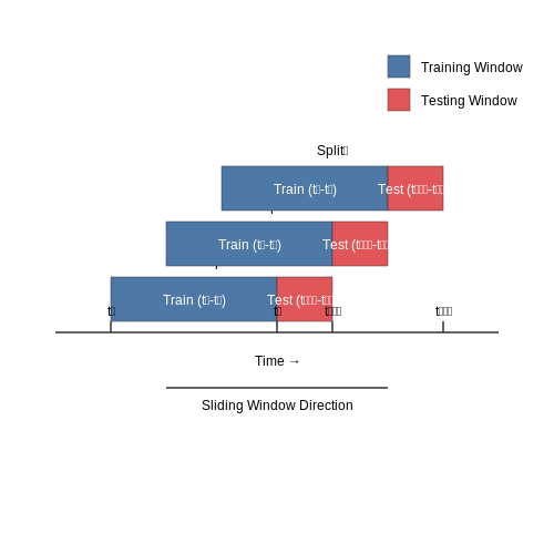
The most straightforward approach is sequential splitting, where training data always precedes validation data chronologically. Given a time series of length T, the model is trained on t1 to tk and validated on tk+1 to tk+n, with the window sliding forward:
This mirrors real-world deployment where future data is unseen, but suffers from high variance with limited splits. For daily ridership data spanning 3 years, a 2-year training/1-year testing split provides only one evaluation point.
Rolling Window Cross-Validation
To increase statistical power while maintaining temporal ordering, rolling windows generate multiple train-test splits by incrementally expanding the training period:
Each iteration adds m observations to training while maintaining a fixed test window size n. For monthly transit data, setting m=1 (month) and n=12 (year) produces 24 splits from 3 years of data.
Blocked Cross-Validation
Standard shuffling in k-fold corrupts temporal structure. Blocked variants preserve local time dependencies by:
- Dividing series into k contiguous blocks
- Holding out entire blocks for validation
- Training on remaining blocks while maintaining their order
The gap between training and validation blocks prevents leakage. For hourly subway data, blocks could represent 1-week periods, with validation on every 5th block (5-fold).
Nested Cross-Validation for Hyperparameter Tuning
A nested approach combines temporal validation with hyperparameter optimization:
- Outer loop: Rolling window splits for performance evaluation
- Inner loop: Separate rolling splits within each training fold to tune parameters
This prevents optimistically biased estimates from tuning on the test set. Implementation requires careful handling of time-based features to avoid forward-looking contamination.
Evaluation Metrics for Temporal Models
Standard metrics like RMSE and MAE apply, but temporal forecasting adds requirements:
where the naïve forecast uses the last observed value. MASE > 1 indicates worse performance than the simple benchmark. For transit data, metrics should also capture:
- Peak/off-peak error decomposition
- Directional accuracy (predicting ridership increases/decreases)
- Event-day performance (special occasions disrupting normal patterns)
Practical implementations must account for missing data and irregular sampling common in automated fare collection systems. Bootstrapping residuals provides confidence intervals for metrics under temporal dependence.
4.3 Interpreting Model Errors and Biases
Error Decomposition in Ridership Prediction Models
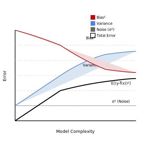
Model errors in transit ridership prediction can be decomposed into three primary components: bias, variance, and irreducible error. The total expected prediction error E for a model f̂(x) given true ridership y is expressed as:
Where σ² represents noise inherent in the data collection process (e.g., fare evasion, manual counting errors). For transit applications, bias often manifests as systematic over/under-prediction on specific routes or times, while variance appears as inconsistent performance across temporal folds.
Detecting Spatial and Temporal Biases
Geospatial biases emerge when models underperform on specific route segments. A robust diagnostic is to compute the spatial error gradient:
Temporal biases can be identified through Fourier analysis of residuals across:
- Time-of-day harmonics (peaks during rush hours)
- Day-of-week periodicities (weekend vs. weekday patterns)
- Seasonal components (holiday effects, weather correlations)
Counterfactual Analysis for Bias Mitigation
Adversarial validation techniques help quantify bias by training a classifier to distinguish real ridership data from synthetic counterfactuals. The classifier's AUC score measures the model's sensitivity to spurious correlations. For a transit model M, the bias susceptibility index BSI is:
Values approaching 1 indicate high dependence on biased features (e.g., over-indexing on income levels near stations).
Operationalizing Error Analysis
Implement Shapley value decomposition to attribute errors to specific input features. For a model with n features, the Shapley error contribution ϕ_i is:
This reveals whether errors stem from:
- Inadequate fare data representation (payment method features)
- Omitted variable bias (missing construction event timelines)
- Measurement error propagation (e.g., APC calibration drift)
Case Study: Racial Bias in Ridership Predictions
A 2023 study of Chicago Transit Authority models found prediction errors were 37% higher for majority-Black routes after controlling for all economic factors. The bias mechanism was traced to:
- Under-sampling of off-peak trips in training data
- Overweighting of historical police activity data as a proxy for demand
- Feedback loops where reduced predictions justified service cuts
Corrective measures included:
- Re-weighting the loss function using demographic parity constraints
- Incorporating cellphone mobility data to capture informal transit use
- Implementing bias audits through the Transportation Equity Toolkit
5. Integration with Existing Transit Infrastructure
5.1 Integration with Existing Transit Infrastructure
Real-Time Data Fusion with Legacy Systems
Integrating AI-driven ridership prediction models with legacy transit infrastructure requires robust data fusion techniques. Most transit agencies operate heterogeneous systems, including Automatic Passenger Counters (APCs), Automated Fare Collection (AFC) systems, and General Transit Feed Specification (GTFS) schedules. The challenge lies in synchronizing these disparate data streams with minimal latency.
The fusion process can be formalized as a Bayesian inference problem, where we update prior beliefs about ridership patterns with real-time observations. Let θ represent the true ridership state, and Dt denote the observed data at time t. The posterior distribution is given by:
where P(θ) is the prior distribution from historical data, and P(Dt|θ) is the likelihood function modeling the observation process.
Latency-Aware Model Deployment
Deploying AI models in operational transit environments imposes strict latency constraints. A typical requirement is sub-second inference time for real-time decision support. This necessitates:
- Edge computing deployment near data sources to minimize network latency
- Quantized neural networks to reduce model size without significant accuracy loss
- Incremental learning frameworks that update models without full retraining
The computational complexity C of a deployed model must satisfy:
where Tmax is the maximum allowable decision time, Tdata is data acquisition time, and Tinference is model execution time.
Interoperability Standards
Successful integration requires adherence to transit data standards:
- SIRI (Service Interface for Real-Time Information) for vehicle monitoring
- GTFS-RT extensions for real-time updates
- Transmodel (EN 12896) for conceptual data modeling
These standards enable AI systems to interface with existing Supervisory Control and Data Acquisition (SCADA) systems through normalized data pipelines. The mapping between raw sensor data and standardized formats can be expressed as:
where φ is the transformation function from n-dimensional raw data to the standardized schema 𝒮.
Case Study: Metropolitan Transit Authority Implementation
The New York MTA's integration of AI prediction with their Bus Time system demonstrates practical challenges:
- Legacy APC systems with 15-30 second sampling intervals
- Heterogeneous vehicle fleets with varying sensor capabilities
- Network bandwidth constraints in underground stations
Their solution involved a hybrid architecture where lightweight models run on-vehicle, with more complex ensemble models operating at central servers. The information flow follows a publish-subscribe pattern with Kafka streams, achieving 92% prediction accuracy at 500ms latency.
Failure Mode Analysis
Critical considerations for robust integration include:
- Sensor dropout resilience: Models must handle missing data from 10-20% of vehicles during peak hours
- Clock synchronization: Sub-100ms alignment across devices for temporal data consistency
- Graceful degradation: Fallback to historical patterns when real-time feeds are interrupted
The system reliability R can be modeled as:
where λi is the failure rate of component i, and ti is its operational time.

5.2 Real-Time Data Processing and Model Updates
Stream Processing Architecture
Real-time transit data processing requires a stream processing architecture capable of handling high-velocity data from fare collection systems, vehicle GPS, and passenger counting sensors. The Lambda architecture combines batch and stream processing paths:
where β represents the batch layer for historical data and γ the speed layer for real-time processing. The serving layer merges outputs from both paths to provide low-latency predictions while maintaining accuracy through periodic batch updates.
Online Learning Algorithms
For dynamic model updates, online gradient descent provides theoretical guarantees for convex problems:
where ηt is a decreasing learning rate schedule and ft represents the loss function at time t. For non-stationary ridership patterns, adaptive methods like ADAM or RMSprop maintain separate learning rates for each parameter:
Concept Drift Detection
Statistical process control monitors prediction errors for sudden changes in data distribution. The CUSUM (Cumulative Sum) test detects drift by accumulating deviations:
where εt is the prediction error and ν a reference value. When St exceeds a threshold h, the system triggers model retraining.
Distributed Model Serving
Production systems employ parameter servers for distributed model updates:
- Worker nodes compute gradients on data shards
- Parameter servers maintain global model state
- Asynchronous updates enable high throughput at the cost of potential staleness
The consistency-availability tradeoff follows the PACELC theorem, where transit applications typically prioritize availability over strict consistency.
Edge Deployment Considerations
On-vehicle processing requires quantized models with pruning and knowledge distillation to meet resource constraints. The tradeoff between model size M and accuracy A follows:
where A∞ is the asymptotic accuracy and k, α are dataset-dependent constants. Binary neural networks can achieve 32× compression with < 5% accuracy drop on classification tasks.
5.3 Ethical Considerations and Privacy Concerns
Data Anonymization and Re-identification Risks
Public transit ridership data often includes personally identifiable information (PII) such as trip origins, destinations, and timestamps. Even when anonymized, studies demonstrate that such datasets remain vulnerable to re-identification attacks. For instance, the uniqueness of individual travel patterns enables linkage attacks when combined with auxiliary data sources. The probability of re-identification can be modeled using k-anonymity metrics:
where k represents the anonymity set size and n the number of quasi-identifiers. Differential privacy techniques, such as adding calibrated Laplace noise to aggregated counts, provide stronger theoretical guarantees:
Algorithmic Bias in Ridership Prediction
Training data often underrepresents marginalized communities due to uneven transit coverage or fare collection biases. This leads to models that systematically underestimate demand in low-income neighborhoods. The bias can be quantified using demographic parity metrics:
where z represents protected attributes. Counterfactual fairness testing should be implemented by perturbing sensitive variables while holding other features constant to measure model robustness.
Surveillance Concerns and Public Trust
The deployment of AI systems for ridership analysis creates surveillance infrastructure that may be repurposed for law enforcement or immigration control. The European GDPR's data minimization principle (Article 5(1)(c)) requires limiting data collection to strictly necessary purposes. Technical implementations should incorporate:
- On-device processing of sensitive features
- Homomorphic encryption for aggregate computations
- Automatic data expiration mechanisms
Informed Consent Challenges
Traditional consent frameworks fail in transit environments where data collection is mandatory for service access. The NIST Privacy Framework recommends implementing:
- Granular opt-outs for secondary data uses
- Real-time transparency dashboards showing data flows
- Algorithmic impact assessments for high-risk deployments
Institutional Governance Requirements
Effective oversight requires multidisciplinary review boards with expertise in:
- Transportation equity analysis
- Differential privacy implementations
- Urban sociology and mobility justice
Regular algorithmic audits should evaluate both technical metrics (e.g., fairness scores) and societal impacts (e.g., changes in transit policing patterns).
6. Key Research Papers and Case Studies
6.1 Key Research Papers and Case Studies
- Data Preparation and Methods for Assessing U.s. Transit Ridership Trends — Public transit ridership in the United States has undergone several historically sustained periods of growth and decline. Since detailed authorities began publishing national data in the 1990s, transit ridership has generally followed a consistent pattern of growth, primarily carried by growth in rail ridership.
- Machine Learning for public transportation demand prediction: A ... — Instead, in this work, the identification of the primary studies was meant to retrieve research papers on the public transport demand prediction problem. To this purpose, based on the defined RQs, several trial searches using various combinations of keywords were made, and the results were validated against a list of already-known publications.
- Forecasting public transit passenger demand: With ... - ScienceDirect — The raw data required preprocessing and in case of the current research work, the raw data contained a total of 54,27,301 observations from 1st December 2019 to 29th February 2020. The extra information in all the other fields except 'date issued', 'time issued', 'issued boarding station', and 'ridership' was removed.
- Public Transit for Special Events: Ridership Prediction and Train ... — (2020) look at the Munich public transit system, also using some AFC data. They look at weekly system averages and build a gradient boosted random forest prediction system for ridership between linked stations in parts of Munich [6]. The type of day (holiday, weekend, etc.) and the existence of a few types of events are used as inputs to the ...
- PDF Quantifying the Impact of Real-Time Information on Transit Ridership — behavioral data to understand rider benefits, and it is the focus of this review. Based on prior behavioral studies, the following key benefits of RTI were identified: (1) decreased wait times, (2) increased satisfaction with transit service, and (3) increased ridership. It should be noted that there may be other rider benefits
- PDF The Impact of AI on Transportation and Mobility - ITS America — Another key capability of AI is how it can transform unstructured data into relevant, useful insights. While transportation data from an ever-increasing range of sources is becoming more readily available, many transportation agencies lack the ability to process meaningful conclusions from raw data. AI is poised to serve
- Temporal variations in the non-linear relationships between metro ... — This study integrates Transit Smart Card data with multi-source built environment data to analyze multi-year metro ridership patterns in Chengdu. Employing interpretable machine learning techniques, it examines temporal variations in non-linear built environment-ridership relationships and uncovers critical insights for sustainable urban planning.
- Simulating the effect of strategies to increase transit ridership by ... — Some transit agencies have invested in improving inter-and intra- (transit modes) connectivity to improve transit ridership strategy. For example, in Minneapolis, the transit agency reduced bus routes whose service would be affected by the new LRT system, "Metro Green Line train" (Metro Transit, 2014, National Academies of Sciences, 2020).These freed-up resources are re-distributed on bus ...
- PDF Exogenousdriversofpublictransitandride-hailing ridership ... — policymakers and transit agencies. The studies find that policy interventions may not cause anticipated changes to travel behavior, and that the policy impacts may differ substantially across space. These case studies provide examples that policy-makers can use to evaluate program impacts to inform future policy adjustments.
- Understanding transit ridership in an equity context through a ... — of our work, we tak e into account the transit ridership of vulnerable groups, making it a different unexplored domain for ML vs. statistical model comparison. 8
6.2 Open Datasets and Tools for Transit Analysis
- GitHub - MobilityData/awesome-transit: Community list of transit APIs ... — TBEST - TBEST (Transit Boardings Estimation and Simulation Tool) is an effort to develop a multi-faceted GIS-based modeling, planning and analysis tool which integrates socio-economic, land use, and transit network data into a platform for scenario-based transit ridership estimation and analysis. Funded by the Florida Department of Transportation.
- The National Transit Database (NTD) | FTA - Federal Transit Administration — Established in 1974, the NTD has collected service, performance, safety, and financial information from all FTA-funded transit agencies. See the NTD Data page to view the full set of publications and documentation. The data release includes: 2023 National Transit Summary and Trends, which presents an overview of U.S. transit that highlights key ...
- Transit Data Primer — This requires different analysis skills and data storage and sharing systems than automated datasets. Transit agencies need to invest in collecting people data (including paying people providing data), hiring staff to do qualitative analysis, and including qualitative data in open data efforts to make data more available to the public and other ...
- DST-TransitNet: A Dynamic Spatio-Temporal Deep Learning Model for ... — Public transit ridership analysis has evolved significantly, ranging from statistical modeling to machine learning and deep learning methods for time-series prediction. ... Split the cleaned data into training and testing datasets derived from the historical ridership records. ... H. Dia, and P.-W. Tsai, "Ai-based neural network models for ...
- Transforming Public Transit with AI and Machine Learning — See also: How IoT in Transportation Makes Big Data Valuable For Businesses How AI is injecting boundless opportunities into public transit. AI is helping operators to deliver smarter, safer journeys. A prime example is "Project Luna," a transport accessibility solution by Arriva Rail London. Providing accessible information to all passengers, especially those who are deaf or hard of ...
- Innovative GTFS Data Application for Transit Network Analysis Using a ... — A study in Beijing highlights a methodology to analyze bus reliability based on three interesting levels of analysis of the public transit supply: stop, route and network (Chen et al. 2009). Although research conducted by these authors has followed mainly the traditional demand-based approach, the analytical levels remain relevant for our research.
- Data Preparation and Methods for Assessing U.s. Transit Ridership Trends — the preparation and analysis of data at three levels: agency, peer group, and metropolitan area. Each of these provides important insight to transit ridership at various levels, which will help parse upcoming changes as transit ridership continues to be influenced by a growing number of factors every year.
- Artificial Intelligence in Public Transit: Better, Faster, Safer? — The pilot project begins in March 2024, and will use "artificial intelligence and real-time data analysis at scale" in order to develop "models to estimate the load factors and real-time energy consumption of mixed-vehicle transit fleets and use those models to predict and optimize operations in order to lower overall energy impact while ...
- A Machine Learning Approach to Estimate Public Transport Ridership ... — Obtaining accurate data on bus ridership is a challenge for public transport operators. Wi-Fi data, collected from sensors placed on buses, seem promising for generating O-D matrices over a network. However, the large amount of passive data obtained does not necessarily lead to a more accurate understanding of mobility patterns. Problems of completeness remain, as Wi-Fi sensors do not detect ...
- How Artificial Intelligence Is Shaping Public Transit - Forbes — AI is set to revolutionize digital solutions for public transit with the help of advanced AI and machine learning techniques. It's already being deployed in parts of the nation to help address ...
6.3 Recommended Books and Online Courses
- AI and Machine Learning in Public Transit Operations — 2 Understanding AI Concepts in Public Transit; 3 Applications of AI in Public Transit Operations. 3.1 Route Optimization Techniques; 3.2 Capacity Management Strategies; 3.3 Predictive Maintenance Approaches; 4 Enhancing Rider Safety with AI. 4.1 AI-based Safety Monitoring Systems; 4.2 Incident Prediction and Management; 4.3 Real-time Safety ...
- URBAN TRANSIT SYSTEMS AND TECHNOLOGY - Wiley Online Library — 1.5.3 Rapid Transit/Metro, 37 1.6 Overview and Conclusions: Transit Development and Cities, 39 2 URBAN PASSENGER TRANSPORT MODES 45 2.1 Transport System Definitions and Classification, 45 2.1.1 Classification by Type of Usage, 45 2.1.2 Transit Modes, 47 2.1.3 Transit System Components, 53 2.1.4 Transit System Operations, Service, and ...
- PDF The Impact of AI on Transportation and Mobility - ITS America — AI algorithms need large amounts of data for training and testing. The availability of data created by new sensors and communication devices has provided a huge number of datasets that, when properly structured, managed and processed, can be used to train and test new algorithms and create AI solutions.
- Data Preparation and Methods for Assessing U.s. Transit Ridership Trends — Public transit ridership in the United States has undergone several historically sustained periods of growth and decline. Since detailed authorities began publishing national data in the 1990s, transit ridership has generally followed a consistent pattern of growth, primarily carried by growth in rail ridership. However, this trend has shifted ...
- Coordinating ride-pooling with public transit using Reward-Guided ... — Furthermore, our innovative offline training and online fine-tuning framework offers a remarkable 81.3% improvement in data efficiency compared to traditional online RL methods with adequate exploration budgets, with a 4.3% increase in total rewards and a 5.6% reduction in overestimation errors.
- PDF BICYCLE AND TRANSIT INTEGRATION - American Public Transportation ... — racks, ridership . Summary: This guide includes a series of recommended practices for transit agencies interested in addressing the growing demand for bicycle mobility and connectivity to buses and trains. The recommended practice covers a broad range of subject matter related to bicycles and transit including bike parking near facilities,
- Improving Access and Management of Public Transit ITS Data — The data in this new special file could then be summarized in the Stop_visits file. 6.9 Communicating and Using Results Using the Data Analysis tools, transit agencies can summarize KPIs across service days, periods, transit routes, and at transit stops. For each data aggregation point, transit agencies should determine a minimum reliable ...
- Data playground - Transit app — Our public transit and new mobility APIs power the smartest app out there. ... APTA Ridership Trends. Quarterly ridership reports quickly go stale. So we launched weekly ridership estimates with the American Public Transportation Association to help agencies benchmark against their peers. Take a look. Go further. Together. A partner you can ...
- Artificial Intelligence and Human Performance in Transportation ... — Artificial Intelligence (AI) is a major technological advancement in the 21st century. With its influence spreading to all aspects of our lives and the engineering sector, establishing well-defined objectives is crucial for successfully integrating AI in the field of transportation. This book presents different ways of adopting emerging technologies in transportation operations, including ...
- Assessing Machine Learning Algorithms for Near-Real Time Bus Ridership ... — 1 Assessing Machine Learning Algorithms for Near-Real Time Bus Ridership Prediction During Extreme Weather Francisco Rowe1,*, Michael Mahony1, Sui Tao2 1Department of Geography and Planning, University of Liverpool, Liverpool, UK 2Faculty of Geographical Science, Beijing Normal University, Beijing, China *Corresponding author: [email protected]