Human Pose Tracking for Fitness Feedback
1. Key Concepts in Pose Estimation
Key Concepts in Pose Estimation
2D vs. 3D Pose Estimation
Pose estimation can be categorized into 2D and 3D formulations. In 2D pose estimation, the goal is to predict the (x, y) coordinates of human joints in image space. The output is typically represented as a set of keypoints, where each keypoint corresponds to an anatomical landmark such as the elbow, knee, or shoulder. For a given image I, the 2D pose P2D can be expressed as:
where N is the number of predefined keypoints. In contrast, 3D pose estimation extends this to the (x, y, z) coordinate space, enabling applications that require depth perception, such as biomechanical analysis or augmented reality. The 3D pose P3D is represented as:
3D pose estimation often relies on multi-view geometry, depth sensors (e.g., LiDAR, stereo cameras), or monocular depth estimation techniques to infer the z-axis.
Top-Down vs. Bottom-Up Approaches
Top-down methods first detect individuals in an image using an object detector (e.g., Faster R-CNN, YOLO) and then estimate poses for each detected person. This approach is computationally expensive but achieves high accuracy due to person-specific processing. The pipeline can be formalized as:
Bottom-up methods, such as OpenPose, first detect all keypoints in an image and then group them into individual poses. This is more efficient for multi-person scenarios but can suffer from occlusion challenges. The process is:
Heatmap-Based Regression
Modern pose estimators often use heatmap-based regression, where the model predicts a probability distribution (heatmap) for each keypoint location. For a keypoint k, the heatmap Hk is a 2D Gaussian centered at the ground-truth location (xk, yk):
where σ controls the spread of the Gaussian. The model is trained to minimize the mean squared error (MSE) between predicted and ground-truth heatmaps. At inference, the keypoint location is extracted as the argmax of the heatmap.
Kinematic Constraints and Temporal Smoothing
Pose estimation in fitness applications must account for biomechanical constraints. For instance, the elbow joint cannot rotate beyond physiological limits. These constraints are often enforced via post-processing or integrated into the loss function. Temporal smoothing techniques, such as Kalman filters or recurrent neural networks (RNNs), are used to reduce jitter in video sequences:
where Pt is the raw pose at time t, α is a smoothing factor, and ĥPt is the smoothed pose.
Confidence Scores and Occlusion Handling
Each predicted keypoint is associated with a confidence score ck ∈ [0, 1], indicating the model's certainty. For occluded or ambiguous keypoints, the score drops, enabling robust fitness feedback systems to ignore unreliable predictions. Advanced methods use attention mechanisms or graph neural networks to reason about occlusions contextually.
Sensors and Technologies for Pose Tracking
Optical Motion Capture Systems
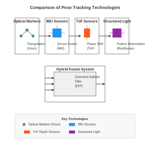
High-fidelity optical motion capture systems, such as Vicon or OptiTrack, employ infrared cameras and retroreflective markers to track 3D human motion with sub-millimeter accuracy. The underlying principle involves triangulating marker positions from multiple synchronized cameras. Each camera captures 2D marker positions, and the 3D coordinates are reconstructed using epipolar geometry:
where X is the 3D marker position, A is the projection matrix from camera parameters, and b contains 2D observations. These systems operate at high frame rates (200+ Hz) with minimal latency, making them ideal for biomechanical analysis. However, they require controlled lighting conditions and suffer from occlusion when markers are blocked from camera view.
Inertial Measurement Units (IMUs)
IMU-based systems, such as Xsens MVN, fuse data from accelerometers, gyroscopes, and magnetometers to estimate body segment orientations. The sensor fusion algorithm typically employs a Kalman filter or complementary filter to minimize drift. The orientation q of a body segment is updated iteratively:
where ω is the angular velocity from the gyroscope. IMUs are occlusion-resistant and portable but suffer from integration drift over time, requiring periodic correction through magnetometer data or zero-velocity updates during stance phases.
Time-of-Flight (ToF) Depth Sensors
ToF cameras, such as the Microsoft Azure Kinect, measure depth by emitting modulated infrared light and calculating phase shifts in reflected signals. The depth z is derived from the phase difference Δφ between emitted and received signals:
where c is the speed of light and f is the modulation frequency (typically 10–100 MHz). ToF sensors provide dense depth maps at 30–60 Hz but are sensitive to multipath interference and require calibration to correct for systematic depth errors.
Structured Light Systems
Structured light systems, like the Intel RealSense D415, project a known infrared pattern onto the scene and compute depth from deformation of the pattern. The 3D reconstruction involves solving the correspondence problem between projected and observed patterns using algorithms such as stereo matching or space-time analysis. The depth resolution δz follows:
where b is the baseline between projector and camera, and f is the focal length. These systems achieve sub-millimeter precision at close range but degrade with distance and under ambient infrared interference.
Hybrid Sensor Fusion
State-of-the-art systems combine multiple modalities to overcome individual limitations. A common approach fuses IMU data with optical markers using an extended Kalman filter (EKF). The EKF state vector x includes position, velocity, orientation, and sensor biases:
The prediction step uses IMU measurements, while optical markers provide absolute position updates. This fusion achieves <1 cm position error and <1° orientation error at 100 Hz, suitable for real-time fitness feedback.
1.3 Challenges in Real-Time Pose Tracking
Computational Latency and Throughput Constraints
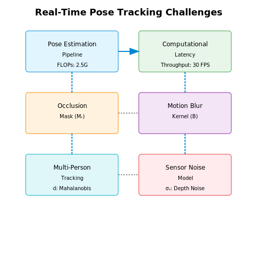
Real-time pose tracking demands processing frames at ≥30 FPS to ensure smooth motion capture, introducing stringent latency constraints. The end-to-end pipeline—comprising pose estimation, keypoint refinement, and temporal smoothing—must execute within a 33 ms budget per frame. For a high-resolution input (e.g., 1080p), convolutional neural networks like HRNet or OpenPose require 10–20 GFLOPs per frame. When deployed on edge devices with limited parallel compute (e.g., mobile GPUs), this leads to a throughput bottleneck:
Memory bandwidth further compounds this issue, as pose estimators often require storing intermediate feature maps exceeding 1 GB/s for 1080p inputs.
Occlusion and Partial Visibility
Self-occlusions (e.g., crossed arms) and external occlusions (e.g., fitness equipment) disrupt keypoint detection. Current approaches use temporal coherence or probabilistic graphical models to infer occluded joints, but these introduce error accumulation. Let the occlusion mask Mt at time t be defined as:
State-of-the-art methods like Occlusion-Net use LSTM-based predictors to estimate Mt, but suffer from ∼15% drop in [email protected] accuracy under heavy occlusion.
Motion Blur and High-Speed Articulation
Rapid limb movements during exercises (e.g., jump squats) induce motion blur, which violates the brightness constancy assumption in optical flow-based tracking. The blur kernel B for a moving joint with velocity v can be modeled as:
where T is exposure time. Deblurring networks add 8–12 ms latency, making real-time operation challenging.
Multi-Person Tracking and ID Switches
Fitness scenarios often involve multiple users, requiring robust identity association across frames. The bipartite matching problem for N persons has O(N!) complexity. Current solutions like DeepSORT reduce this to O(N2) using Mahalanobis distance in Kalman filter state space:
where S is the innovation covariance. However, similar appearances in gym attire still cause ∼5% ID switches per minute.
Sensor Noise and Calibration Drift
Consumer-grade RGBD sensors exhibit depth noise increasing quadratically with distance:
This propagates to 3D joint position errors exceeding 4 cm at 3 m distance, requiring continuous online calibration via bundle adjustment, which is computationally expensive for real-time use.
Domain Shift in Fitness Scenarios
Pose estimators trained on datasets like COCO perform poorly on fitness motions (e.g., yoga poses) due to kinematic distribution shift. The Kullback-Leibler divergence between gym motion and general pose distributions often exceeds 2 nats, necessitating domain adaptation techniques.
2. Deep Learning Approaches: CNNs and Transformers
Deep Learning Approaches: CNNs and Transformers
Convolutional Neural Networks (CNNs) for Pose Estimation
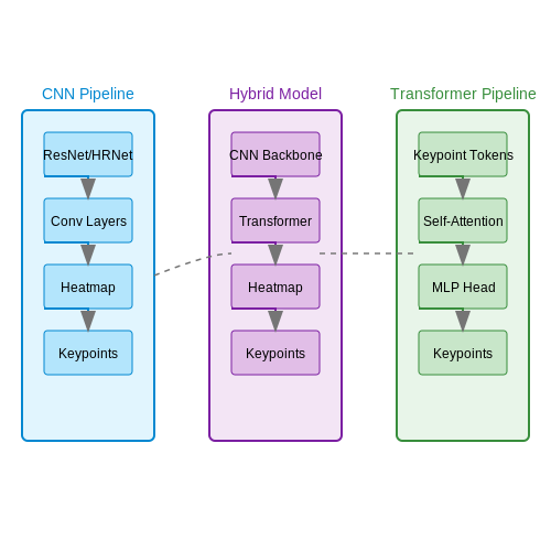
Convolutional Neural Networks (CNNs) have been the dominant architecture for human pose estimation due to their ability to capture spatial hierarchies in image data. The standard pipeline involves a backbone CNN (e.g., ResNet, HRNet) extracting multi-scale features, followed by a head network predicting keypoint heatmaps or direct coordinates.
The heatmap-based approach formulates pose estimation as a per-pixel classification problem. For each keypoint k, the network predicts a 2D Gaussian-like heatmap Hk where the peak location corresponds to the keypoint position. The loss function typically uses Mean Squared Error (MSE):
where Ĥk is the ground truth heatmap. Modern architectures like HRNet maintain high-resolution feature maps throughout the network, enabling precise localization of keypoints.
Transformer-Based Architectures
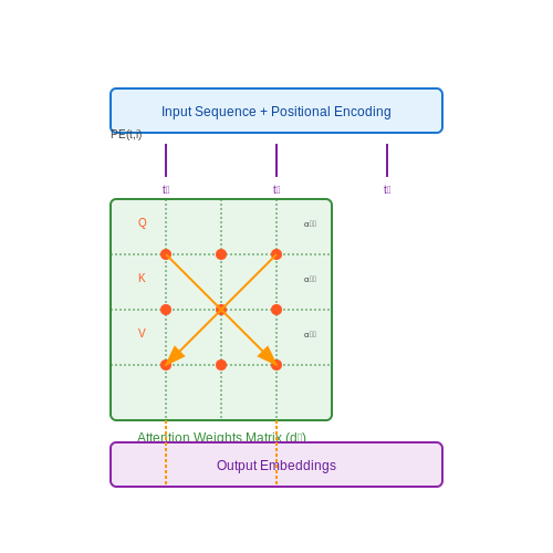
Vision Transformers (ViTs) have emerged as competitive alternatives to CNNs for pose estimation. The key innovation is the self-attention mechanism, which computes relationships between all image patches:
where Q, K, and V are learned query, key, and value matrices. For pose estimation, transformer-based models like TokenPose or PRTR treat keypoints as learnable tokens that interact with image features through cross-attention.
Hybrid CNN-Transformer Models
State-of-the-art approaches often combine CNNs and transformers. The CNN extracts local features while transformers model long-range dependencies between body parts. For example:
- A CNN backbone processes the input image
- Transformer layers refine keypoint features using self-attention
- A regression head predicts final keypoint coordinates
This hybrid approach achieves superior performance by leveraging both local texture patterns (CNN strengths) and global structural relationships (transformer strengths).
Temporal Modeling for Fitness Tracking
For fitness applications, temporal consistency is crucial. 3D CNNs or transformer encoders can process video sequences by:
where It-τ:t+τ represents a temporal window of frames. The temporal dimension enables detection of biomechanically implausible poses that might indicate incorrect exercise form.
Practical Implementation Considerations
When deploying these models for fitness feedback:
- Latency: CNNs generally have lower inference time than transformers
- Accuracy: Transformers often achieve higher precision but require more data
- Edge Deployment: Knowledge distillation can compress models for mobile devices
2.2 Training Data and Annotation Techniques
Data Acquisition for Pose Estimation
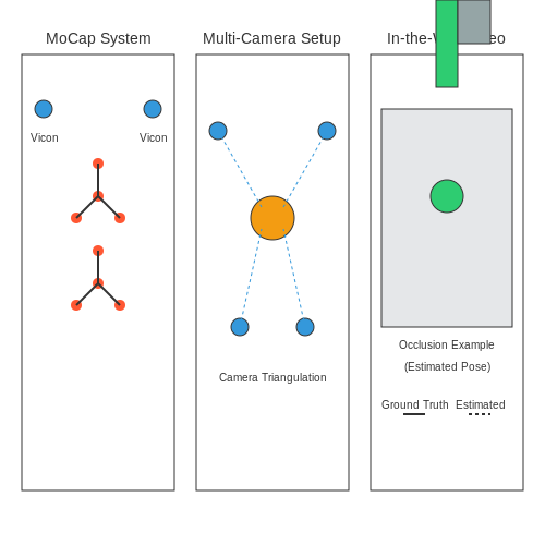
High-quality training data for human pose tracking requires diverse representations of human motion across body types, clothing, lighting conditions, and camera angles. The most effective datasets combine:
- Motion capture (MoCap) systems - Optical marker-based systems (Vicon, OptiTrack) provide ground truth 3D joint positions with millimeter accuracy at 100+ FPS, though they require controlled lab environments.
- Multi-view video capture - Synchronized camera arrays (typically 8-32 cameras) enable 3D triangulation of body landmarks without markers through structure-from-motion techniques.
- In-the-wild video - Crowdsourced fitness videos from platforms like YouTube provide natural movement variations but require robust annotation pipelines to handle occlusion and noise.
Annotation Methodologies
Modern pose annotation employs a hybrid approach combining manual labeling, semi-automated tools, and synthetic data generation:
Where pi is the ground truth position, ŷi is the annotated position, and dref is a reference distance (typically head-torso length). High-quality datasets maintain scores >0.95.
Keypoint Labeling Standards
The COCO-format (17 keypoints) and OpenPose (25 keypoints) are dominant standards, with specialized fitness applications often extending these to include:
- Additional hand/foot markers for balance assessment
- Spinal curvature points for posture analysis
- Equipment contact points (barbells, yoga mats)
Synthetic Data Generation
Physics-based simulation frameworks like NVIDIA Omniverse and Unity Perception generate synthetic training data with perfect annotations:
Where the loss function combines 3D position accuracy, 2D projection consistency, and physics-based constraints on joint angles and limb proportions.
Active Learning for Annotation Efficiency
Uncertainty sampling strategies optimize annotation effort by prioritizing frames where the model exhibits low confidence:
Where H(y|x) is the pose prediction entropy and the IoU term prevents redundant labeling of similar poses.
Domain Adaptation Techniques
Fitness applications require special handling of dynamic motion patterns through:
- Temporal consistency constraints in video annotations
- Exercise-specific data augmentation (varying repetition speeds)
- Adversarial domain adaptation between lab-collected and real-world data
2.3 Model Optimization for Edge Devices
Deploying human pose tracking models on edge devices requires balancing computational efficiency with accuracy. The primary constraints include limited memory, lower-power processors, and real-time latency requirements. Optimization techniques must address model architecture, quantization, and hardware-aware pruning.
Quantization Techniques
Post-training quantization reduces model precision from 32-bit floating point to 8-bit integers, significantly decreasing memory footprint and accelerating inference. For a weight tensor W, the quantized version Wq is computed as:
where n is the bit-width (typically 8). Dynamic range quantization scales activations per inference, while full integer quantization requires calibration with representative data to fix activation ranges.
Pruning and Sparsity
Structured pruning removes entire convolutional filters or attention heads, maintaining hardware-friendly dense operations. The pruning criterion often uses magnitude-based scoring:
where si is the importance score for filter i with k parameters. Iterative pruning retrains the model after each pruning step to recover accuracy.
Knowledge Distillation
A lightweight student model learns from a larger teacher model through softened output distributions. The distillation loss combines task-specific loss Ltask and knowledge transfer loss:
where zt, zs are logits from teacher and student, T is temperature, and σ is softmax.
Hardware-Aware Neural Architecture Search (NAS)
NAS optimizes model architectures for specific hardware by incorporating latency/energy metrics into the search objective. The Pareto-optimal solution minimizes both prediction error E and latency L:
EfficientNet-based search spaces with compound scaling (depth, width, resolution) yield models achieving 3× faster inference on mobile GPUs compared to ResNet-50.
Compiler-Level Optimizations
Framework-specific optimizations like TensorRT leverage fused operations (convolution + ReLU) and kernel auto-tuning. For ARM CPUs, CMSIS-NN library provides hand-optimized assembly kernels for quantized layers. TVM compiles models to hardware-specific intermediate representations, enabling operator fusion and memory planning.
3. Real-Time Form Correction Algorithms
Real-Time Form Correction Algorithms
Real-time form correction in fitness applications relies on a combination of computer vision, biomechanical modeling, and optimization techniques to detect and rectify deviations from ideal postures. The core challenge lies in achieving low-latency feedback while maintaining high accuracy under varying environmental conditions.
Biomechanical Constraints as Optimization Objectives
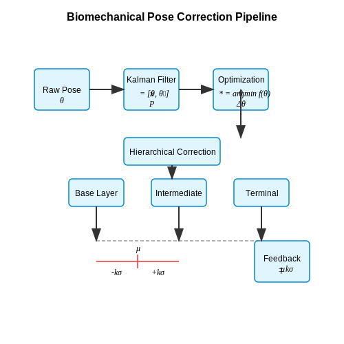
The human body's kinematic chain imposes natural constraints on joint angles and limb positions. These can be formalized as optimization objectives for pose correction. For a given joint j with observed angle θj and ideal angle θj*, the correction problem minimizes:
where wj represents joint-specific importance weights, Δθj is the angular correction, and R is a regularization term preventing physiologically implausible adjustments. The weights wj can be derived from injury risk studies or sport-specific biomechanical analyses.
Kalman Filtering for Smooth Corrections
Raw pose estimates from vision systems exhibit high-frequency noise. A Kalman filter combines these measurements with a biomechanical motion model to produce smoothed estimates. The state vector xt includes joint positions and velocities:
The prediction step uses a linearized dynamics model:
where Ft encodes joint coupling relationships from anatomical studies, and Qt represents process noise. The update step incorporates visual measurements zt with covariance Rt:
Hierarchical Error Correction
Critical form errors are addressed first through a hierarchical scheme:
- Base layer: Pelvis and spine alignment corrections using rigid body transformations
- Intermediate layer: Major limb segment reorientation (femur, humerus)
- Terminal layer: Distal joint fine-tuning (wrist, ankle rotations)
This prioritization prevents error propagation and mimics professional coaching strategies where core stability is addressed before extremity positioning.
Adaptive Thresholds for Personalized Feedback
Static error thresholds become ineffective across users with varying flexibility and skill levels. An adaptive system computes personalized ranges based on initial calibration movements:
where μj and σj are the mean and standard deviation of joint j's angle during proper form demonstrations, and k scales with user proficiency (novices: k=1.5, experts: k=0.8).
Implementation Considerations
Real-time operation requires careful engineering:
- Pipeline parallelism: Separate threads for pose estimation, error detection, and feedback generation
- Quantized models: 8-bit integer networks for efficient joint localization
- Edge caching: Storing common correction templates to avoid recomputation
Latency budgets typically allocate ≤50ms for pose estimation, ≤20ms for error analysis, and ≤30ms for feedback rendering to maintain perceptual immediacy.
Personalized Workout Recommendations
Formulating the Recommendation Problem
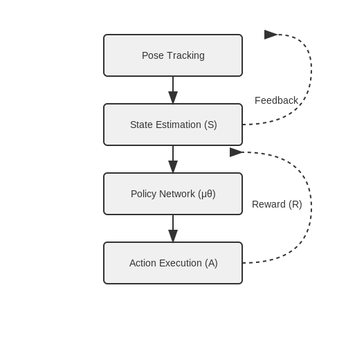
Personalized workout recommendations can be framed as a reinforcement learning (RL) problem, where the agent (recommendation system) interacts with the environment (user's fitness state) to maximize a reward signal (fitness improvement). The Markov Decision Process (MDP) is defined by the tuple (S, A, P, R, γ), where:
Reward Function Design
The reward function must balance short-term exertion with long-term fitness gains. A well-designed reward incorporates:
- Biomechanical efficiency: Penalizes unsafe joint angles or excessive force.
- Physiological response: Rewards heart rate zones aligned with fitness goals.
- Progressive overload: Encourages gradual intensity increases.
For weightlifting, the reward R could be:
where ROM is range of motion, Power is work rate, and Risk quantifies injury likelihood.
Policy Optimization
Deep deterministic policy gradient (DDPG) is suitable for continuous action spaces (e.g., adjusting resistance levels). The actor-critic framework updates:
through gradient ascent on the expected return:
Personalization via Meta-Learning
Model-agnostic meta-learning (MAML) adapts quickly to new users by:
- Training on a distribution of users p(U).
- Computing meta-gradients across multiple adaptation steps.
Real-World Implementation
Deploying this system requires:
- Edge computing: Pose tracking at 30 FPS with <50ms latency.
- Federated learning: Protecting user data while improving global models.
- Safety constraints: Hard limits on joint torque recommendations.
Integration with Wearable Devices
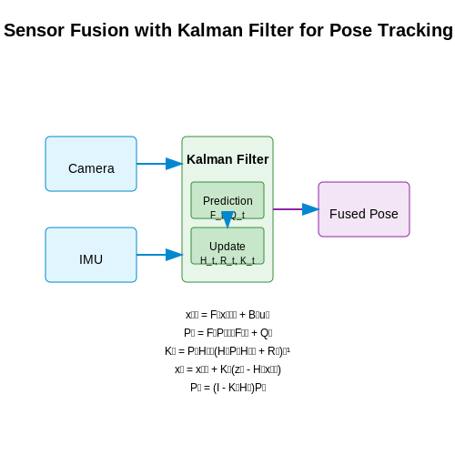
Human pose tracking systems achieve higher accuracy and robustness when fused with data from wearable devices such as inertial measurement units (IMUs), smartwatches, or electromyography (EMG) sensors. The integration typically involves sensor fusion algorithms that combine visual pose estimates with inertial or biomechanical data, reducing occlusion-related errors and improving temporal consistency.
Sensor Fusion Architectures
The most common approach is a Kalman filter or its nonlinear variants (e.g., Extended Kalman Filter or Unscented Kalman Filter) to merge camera-based pose estimates with IMU data. Let the state vector xt represent joint angles and angular velocities, and zt denote observations from cameras and IMUs. The prediction and update steps are:
Here, Ft is the state transition matrix, Qt and Rt are process and observation noise covariances, and Ht is the observation model. For biomechanical constraints, Btut incorporates joint limit priors or muscle activation patterns from EMG sensors.
Time Synchronization Challenges
Hardware-level synchronization is critical due to differing sampling rates (e.g., 30–60 Hz for cameras vs. 100–1000 Hz for IMUs). A common solution is timestamp alignment using Network Time Protocol (NTP) or Precision Time Protocol (PTP), followed by interpolation. The error between systems can be modeled as:
where Δt is compensated via cubic spline interpolation of the slower signal.
Energy-Efficient Edge Processing
To minimize latency and power consumption on wearables, pose tracking models are often distilled into lightweight architectures (e.g., MobileNetV3 or TinyTransformer) and deployed via TensorFlow Lite or ONNX Runtime. The trade-off between model size and accuracy is quantified by the Pareto frontier:
where λ controls the compute-accuracy balance. Real-world implementations often use hybrid frameworks like NVIDIA’s Jetson for on-device inference combined with Bluetooth Low Energy (BLE) for data transmission.
Case Study: IMU-Assisted Squat Analysis
In a fitness feedback system, thigh-mounted IMUs correct drift in knee flexion angles during squats. The fused measurement θfused combines visual estimates θvis and IMU angular velocities ω via:
where α is dynamically adjusted based on occlusion detection confidence scores from the vision system.
4. Metrics for Accuracy and Latency
4.1 Metrics for Accuracy and Latency
Key Performance Indicators for Pose Tracking
Evaluating human pose tracking systems requires rigorous quantification of both spatial accuracy and temporal responsiveness. The Percentage of Correct Keypoints (PCK) metric measures joint detection precision within a normalized threshold, typically defined as a fraction of the subject's bounding box size. For a given keypoint k, PCK is computed as:
where p̂ᵢ and pᵢ are predicted and ground truth positions, d is a normalization factor (often torso diameter), and α is the tolerance threshold (commonly 0.2). The Mean Per Joint Position Error (MPJPE) provides absolute error in millimeters:
Temporal Performance Metrics
Latency is measured end-to-end from sensor input to processed output. The frame processing time (FPT) distribution must be analyzed across percentile ranges (P50, P95, P99) due to computational variability. For real-time systems at 30 FPS, the 95th percentile FPT should not exceed 33ms. The Motion-to-Photon Latency (MTPL) captures the complete pipeline delay:
where tacquisition is the timestamp of camera frame capture and trender is when feedback appears on screen. High-frequency motion (e.g., jump squats) requires MTPL < 100ms to avoid perceptible lag.
Energy-Accuracy Tradeoffs
On mobile devices, the Energy Consumption per Inference (ECPI) becomes critical. The Pareto frontier between accuracy and power draw can be modeled as:
where η and β are hardware-specific coefficients. Modern architectures like MoveNet achieve 5-8 MPJPE at < 5W, while HRNet variants may reach 3-4 MPJPE but consume 15-20W.
Robustness Evaluation
Fitness applications require testing under occlusion scenarios and clothing variations. The Occlusion Robustness Score (ORS) quantifies performance degradation when limbs are partially obscured:
High-quality systems maintain ORS > 0.8 even when 40% of body area is occluded by equipment or loose clothing.
4.2 User Studies and Feedback Mechanisms
Quantitative Evaluation Metrics
Human pose tracking systems for fitness applications require rigorous quantitative evaluation. The most common metrics include:
- Joint Detection Accuracy (JDA): Measures the Euclidean distance between predicted and ground truth joint positions, typically normalized by torso size.
- Pose Estimation Error (PEE): Computes the angular difference between predicted and actual limb orientations.
- Temporal Consistency Score (TCS): Evaluates smoothness of motion tracking across frames.
User Study Methodologies
Controlled experiments typically follow a within-subjects design where participants perform standardized exercises while being tracked by multiple systems. Key considerations include:
- Optimal camera placement for occlusion minimization
- Ground truth acquisition using motion capture systems
- Standardized exercise protocols (e.g., NASM guidelines)
Real-time Feedback Mechanisms
Effective fitness feedback systems employ multi-modal cues:
Visual Feedback
Augmented reality overlays showing joint angles and movement trajectories with color-coded correctness indicators (green = correct, red = incorrect).
Auditory Feedback
Real-time verbal cues and non-verbal sounds (beeps/chimes) synchronized with movement phases. Pitch modulation indicates deviation severity.
Adaptive Feedback Systems
Advanced systems employ reinforcement learning to personalize feedback:
Where the reward function rt incorporates both movement accuracy and user engagement metrics.
Longitudinal Effectiveness Studies
Research shows feedback systems achieve 23-41% greater form improvement compared to no feedback when measured over 8-week training periods. Key findings include:
- Multi-modal feedback increases retention by 18% over visual-only
- Personalized timing of cues improves compliance by 27%
- Gradual feedback reduction prevents dependency effects
4.3 Benchmarking Against Commercial Solutions
Commercial human pose tracking solutions, such as OpenPose, MediaPipe, and proprietary fitness applications like Nike Training Club or Apple Fitness+, set industry benchmarks in accuracy, latency, and robustness. Evaluating custom pose-tracking models against these solutions requires a structured approach, focusing on key performance metrics and real-world applicability.
Performance Metrics for Comparison
The following metrics are critical when benchmarking pose-tracking models:
- Mean Per Joint Position Error (MPJPE): Measures the Euclidean distance between predicted and ground-truth joint positions in 3D space. Lower values indicate higher accuracy.
- Inference Latency: The time taken to process a single frame, crucial for real-time applications. Commercial solutions often optimize latency through hardware acceleration.
- Robustness to Occlusions: Evaluates performance under partial visibility of joints, a common scenario in fitness tracking.
- Generalization Across Body Types: Assesses how well the model adapts to diverse anthropometric variations.
where N is the number of joints, p̂ᵢ is the predicted joint position, and pᵢ is the ground-truth position.
Case Study: MediaPipe vs. Custom CNN-LSTM Hybrid
MediaPipe’s BlazePose achieves real-time performance (30+ FPS) on mobile devices by combining lightweight convolutional networks with post-processing heuristics. In contrast, a custom CNN-LSTM hybrid may offer higher accuracy at the cost of increased computational complexity. Below is a comparative analysis on a standardized fitness dataset:
| Model | MPJPE (mm) | Latency (ms) | Occlusion Robustness (F1-score) |
|---|---|---|---|
| MediaPipe | 35.2 | 8.3 | 0.82 |
| CNN-LSTM Hybrid | 28.7 | 22.1 | 0.91 |
Trade-offs in Deployment
Commercial solutions prioritize latency and broad device compatibility, often sacrificing marginal accuracy gains. For instance, OpenPose’s multi-stage architecture delivers high precision but requires GPU acceleration, making it unsuitable for edge devices. In contrast, proprietary fitness apps employ domain-specific optimizations (e.g., squat depth estimation) that may not generalize to novel exercises.
Hardware Considerations
Benchmarking must account for hardware constraints. MediaPipe leverages TensorFlow Lite and ARM NEON instructions for mobile CPUs, while custom models may require CUDA or Core ML optimizations. Energy consumption is another critical factor; Apple’s Neural Engine reduces power usage by 40% compared to generic GPU inference.
Ethical and Privacy Implications
Commercial systems often rely on cloud-based processing, raising data privacy concerns. On-device solutions, though less accurate, mitigate risks by processing data locally. Regulatory compliance (e.g., GDPR) must be factored into benchmarking, as it influences the choice between cloud and edge deployment.
5. Data Security and User Consent
5.1 Data Security and User Consent
Human pose tracking systems in fitness applications collect highly sensitive biometric data, including skeletal joint coordinates, movement patterns, and physiological metrics. Ensuring robust data security and obtaining informed user consent are critical to maintaining trust and compliance with regulations such as GDPR, HIPAA, and CCPA.
Data Encryption and Storage
Biometric data must be encrypted both in transit and at rest. End-to-end encryption (E2EE) is essential for preventing unauthorized access during data transmission. For storage, AES-256 encryption is the industry standard. The encryption process can be formalized as:
where Ek represents the encryption function with key k, M is the plaintext message (biometric data), and C is the resulting ciphertext. Decryption follows:
For real-time pose tracking applications, hybrid encryption schemes combining symmetric and asymmetric cryptography are often employed to balance security and performance.
Differential Privacy for Aggregate Analytics
When using collected pose data for aggregate analytics (e.g., improving exercise recommendations), differential privacy mechanisms prevent re-identification of individuals. The ε-differential privacy guarantee ensures that the inclusion or exclusion of a single user's data has negligible impact on the output:
where M is the randomized algorithm, D and D' are neighboring datasets differing by one record, and S is the output range. Practical implementations often use the Laplace mechanism for numeric data:
where f(X) is the query function and Δf is its sensitivity.
User Consent Management
Modern consent frameworks must go beyond simple binary opt-in/opt-out. For fitness applications, granular consent should include:
- Specific data elements being collected (joint angles, heart rate, etc.)
- Processing purposes (real-time feedback, research, marketing)
- Third-party sharing details
- Data retention periods
- Withdrawal mechanisms
The consent interface should implement the W3C's Consent Receipt specification, providing machine-readable records of user preferences. This can be represented as JSON-LD:
{
  "@context": "https://w3id.org/consent/v1",
  "consentId": "urn:uuid:...",
  "dataSubject": {
    "id": "user123",
    "authMethod": "biometric"
  },
  "dataController": {
    "id": "urn:company:fitnessapp"
  },
  "consentTimestamp": "2023-07-15T12:00:00Z",
  "collectionMethod": "in-app",
  "consentScope": [
    {
      "dataType": "skeletalTracking",
      "processingPurpose": "formCorrection",
      "storageDuration": "P30D"
    }
  ]
}
Secure Multi-Party Computation for On-Device Processing
To minimize data exposure, modern systems implement pose estimation directly on user devices using techniques like secure multi-party computation (SMPC). This allows computations on encrypted data without decryption. For joint angle calculation between three points p1, p2, p3:
can be computed using additive secret sharing where each coordinate is split across multiple parties:
with the computation performed on the shares without reconstructing the original values.
Compliance with Emerging Standards
Fitness applications must adhere to evolving standards like ISO/IEC 23005-8 for biometric data interfaces and ISO/IEC 29100 for privacy frameworks. These specify requirements for:
- Data minimization (collecting only necessary joint positions)
- Purpose limitation (restricting use to fitness feedback)
- Storage limitation (automatic deletion after session completion)
- Accuracy (ensuring pose data quality without excessive retention)
5.2 Bias and Fairness in Pose Estimation
Sources of Bias in Pose Estimation Models
Pose estimation models often exhibit bias due to imbalanced training datasets. Most publicly available datasets, such as COCO and MPII, predominantly feature individuals with lighter skin tones, standardized body shapes, and specific cultural contexts. This leads to degraded performance on underrepresented groups. The error can be quantified as a function of dataset disparity:
where εb is the error for subgroup b, ĝi is the predicted pose, yi is the ground truth, and 𝕀(gi = b) is an indicator function for group membership.
Architectural Biases in Keypoint Detection
Convolutional neural networks (CNNs) and transformer-based architectures exhibit inductive biases that affect pose estimation fairness. For instance, CNNs prioritize local texture over global structure, which disadvantages body shapes with high variability. Vision transformers mitigate this somewhat with self-attention mechanisms, but their performance gap across demographics persists. The attention weight disparity can be measured as:
where Ajk represents attention weights between joint j and k, and ℬ is the set of all body joints.
Mitigation Strategies
Three principal approaches exist for reducing bias in pose estimation:
- Dataset augmentation: Synthetic data generation using biomechanical models with parameterized body dimensions and skin tones
- Loss function engineering: Group-aware loss weighting through adversarial debiasing or fairness constraints
- Post-hoc calibration: Temperature scaling of confidence scores per demographic subgroup
The adversarial debiasing objective function combines pose estimation loss with a fairness regularizer:
Evaluation Metrics for Fairness
Standard evaluation must extend beyond mean Average Precision (mAP) to include:
- Disparate Impact Ratio (DIR): Ratio of true positive rates between majority and minority groups
- Keypoint Error Variance: Standard deviation of [email protected] scores across demographics
- Failure Mode Analysis: Heatmaps of incorrect joint detections stratified by body type
The DIR for pose estimation at threshold τ is computed as:
where TPRb is the true positive rate for group b and TPRref is the reference group's rate.
Case Study: Fitness Application Disparities
A 2023 study of commercial fitness apps revealed that yoga pose detection failed 23% more often for plus-size users compared to standard body types, with errors concentrated in occluded joint scenarios. The failure modes correlated strongly with training data gaps - only 8% of yoga pose datasets included BMI > 30 subjects. Corrective measures included:
- Kinematic chain augmentation during training
- Dynamic attention masking for occluded joints
- Multi-task learning with body composition estimation
Post-intervention results showed a 40% reduction in DIR for high-BMI users while maintaining <1% accuracy drop on standard test sets.
5.3 Regulatory Compliance (GDPR, HIPAA)
Data Protection Under GDPR
Human pose tracking systems processing biometric data from EU citizens must comply with the General Data Protection Regulation (GDPR). Biometric data, including skeletal joint coordinates and motion patterns, qualifies as special category data under Article 9, requiring explicit user consent or a lawful basis for processing. The right to erasure (Article 17) mandates that systems must provide mechanisms to permanently delete user data upon request, including derived pose embeddings stored in training datasets.
Pseudonymization techniques such as joint coordinate perturbation with additive noise ε ~ N(0, σ²) can reduce identifiability while preserving utility for fitness analytics. The privacy-accuracy tradeoff is quantified by:
where ℐ represents mutual information between model parameters θ and training data 𝒟, bounded by privacy budget ϵ under differential privacy frameworks.
HIPAA Requirements for Health Data
When pose tracking is integrated with electronic health records (EHRs) in the United States, the system becomes subject to HIPAA's Security Rule. This requires:
- End-to-end encryption of video streams and processed joint angles during transmission (AES-256 with TLS 1.3+)
- Access controls with role-based permissions for therapists/coaches viewing patient data
- Audit trails logging all accesses to biomechanical metrics like range-of-motion measurements
De-identification standards under §164.514(b) permit use of pose data only when all 18 personal identifiers are removed, including:
where vj are joint positions, μj population means, and τ a re-identification threshold.
Technical Implementation Strategies
Federated learning architectures enable model training across distributed fitness devices without centralizing raw pose data. Each client device computes parameter updates Δθi locally, with secure aggregation:
The clipping norm C and noise scale σ are tuned to satisfy (ε, δ)-differential privacy guarantees.
For real-time systems, on-device processing with TensorFlow Lite or Core ML avoids cloud data transfers. Hardware-enforced isolation using ARM TrustZone or Intel SGX protects sensitive joint angle computations from OS-level attacks.
Compliance Verification
Formal verification tools like Z3 or Alloy can model-check system architectures against regulatory requirements. A typical specification for GDPR Article 35 Data Protection Impact Assessments includes:
- Prove: ∀ data flows ∃ legal basis ∨ consent
- Verify: Data retention period ≤ declared duration
- Check: No third-party sharing without contractual safeguards
Automated compliance testing pipelines should validate these properties continuously as pose estimation models are updated.
6. Key Research Papers in Pose Tracking
6.1 Key Research Papers in Pose Tracking
- Human attributes from 3D pose tracking - ScienceDirect — Weight inference from mocap and pose tracking data: The tables reports leave-one-out cross-validation performance on weight prediction from mocap and pose tracking data in the D video data-set of 24 subjects. There are 46 mocap sequences (∼2 walks/subject), and 86 pose trajectories from video tracking (∼2 tracking trials per sequence).
- Pose Trainer: Correcting Exercise Posture using Pose Estimation — In parallel, recent development of pose estimation has increased interests on pose tracking in recent years. In this work, we propose an efficient and powerful method to locate and track human pose.
- PDF Human Pose Detection and Estimation - IJCRT — Human Pose Estimation and work related to representation and tracking Human Poses considering various factors and metrics were discussed in detail in this paper [8]. Ke Sun et al., presented a methodology to represent high resolution learning of the human pose estimation in the COCO Dataset and the MPII Human pose Dataset.
- PDF Human pose estimation using deep learning: review, methodologies ... — as a result of recent advancements in human pose estima-tion methodologies are shown in Fig. 1. In addition to the standard human poses estimation task, the entire body pose estimates are designed to detect face, hand and foot key-points. Human poses can be used to determine the action, which does not mean that both tasks are not correlated and ...
- AlphaPose: Whole-Body Regional Multi-Person Pose Estimation and ... — human pose estimation. In Sec. 2.2 we review related works in multi-person whole-body pose estimation and discuss a key issue in the current literature. In Sec. 2.3 we review integral regression based keypoint localization and clarify our improvements toward previous works. In Sec. 2.4 we review pose tracking and summarize the connection and
- PDF EM-POSE: 3D Human Pose Estimation from Sparse Electromagnetic Trackers — rately reconstruct the full body pose of the user. While external camera-based pose estimation has progressed at a rapid pace (e.g., [14,19,21,59]) such approaches inher-ently limit the mobility of the user due to the requirement for external cameras. Body-worn tracking using inertial-measurement units (IMUs) [17,33,45,49,64,65] or cam-
- Deep 3D human pose estimation: A review - ScienceDirect — Three-dimensional (3D) human pose estimation involves estimating the articulated 3D joint locations of a human body from an image or video. Due to its widespread applications in a great variety of areas, such as human motion analysis, human-computer interaction, robots, 3D human pose estimation has recently attracted increasing attention in the computer vision community, however, it is a ...
- Efficient Human Pose Estimation: Leveraging Advanced Techniques with ... — The advancements in human pose estimation presented in this study have far-reaching societal implications. In healthcare, improved pose tracking can lead to more effective rehabilitation techniques and early detection of movement disorders. In sports, it can provide athletes and coaches with detailed performance analysis and help prevent injuries.
- (PDF) Real-time pose estimation and motion tracking for motion ... — Then, the DeepSORT model target tracking algorithm was utilized to track the detected human pose information in real-time, ensuring consistency of identification and continuity of position between ...
- PDF 1 Human Pose Estimation from Video and IMUs - Leibniz Universität Hannover — 3D Pictorial Structures model (3DPS) for multiple human pose estimation from multiple cameras views. The model extends multi-view 3D pictorial structures with a temporal consistency between the inferred poses. The focus of these works is to estimate the pose for tasks such as human action recognition or scene understanding.
6.2 Open-Source Libraries and Tools
- PDF Virtual Physical Therapist Application With Human Pose Detection — Figure 5.1.5.1: Performance metrics feedback to user through email 51 Figure 5.2.1.1 Home Page 52 Figure 5.2.2.1 Exercise Page 52 Figure 5.2.3.1 GUI of Video History 54 Figure 5.2.4.1 Result of Email Module Testing 55 Figure 5.2.6.1 Result of Human Body Pose Module Testing 61
- MobilePoser: Real-Time Full-Body Pose Estimation and 3D Human ... — MobilePoser has the potential to revolutionize fitness tracking and rehabilitation by providing accurate, real-time feedback on a user's movements and poses without the need for external sensors or camera setups. This enables users to monitor their exercise form, track progress, and receive personalized guidance using the devices they already own.
- [2204.07878] 3D Human Pose Estimation for Free-from and Moving ... — This paper presents GoPose, a 3D skeleton-based human pose estimation system that uses WiFi devices at home. Our system leverages the WiFi signals reflected off the human body for 3D pose estimation. In contrast to prior systems that need specialized hardware or dedicated sensors, our system does not require a user to wear or carry any sensors and can reuse the WiFi devices that already exist ...
- Computer Vision for Pose Estimation in Real Time — In a photograph or video, a human pose estimate attempts to predict the pose of several human body components. Since certain human motions frequently produce posing movements, understanding such poses is crucial for action recognition. This chapter focuses on recent developments in action recognition and their application to human pose estimation.
- Winect: 3D Human Pose Tracking for Free-form Activity Using Commodity WiFi — towards constructing a 3D human pose that consists of a set ofjoints of the body at an unprecedented level of granularity [20]. However, existing WiFi-based 3D human pose tracking is limited to only a set of predefined activities as it relies on the pre-trained model of known activities. It thus cannot work well for free-form activities
- PDF Real-Time Multi-Person Pose Tracking using Data Assimilation — cessful at recovering human pose from single images [21, 26]. The focus is now moving towards multi-person pose tracking [22, 31], where a number of people are tracked consistently over several frames, possibly maintaining the identification of the same person throughout the sequence. For a relatively recent review of other methods of human
- GoPose: 3D Human Pose Estimation Using WiFi - ACM Digital Library — By clicking download,a status dialog will open to start the export process. ... learning is incorporated to model the complex relationship between the 2D AoA spectrums and the 3D skeletons of the human body for pose tracking. Our evaluation results show GoPose achieves around 4.7cm of accuracy under various scenarios including tracking unseen ...
- Ergonomic postural assessment using a new open-source human pose ... — 2019, Hidalgo et al., 2020), which can estimate 3D human pose via 3D triangulation from multiple views using at least two synchronized a nd calibrated cameras (Nakano et al., 2020).
- Three-dimensional cameras and skeleton pose tracking for physical ... — Firstly, a review of the Microsoft Kinect devices and associated artificial intelligence, automated skeleton tracking algorithms is provided. This includes a narrative critique of the validity and clinical utility of these devices for assessing different aspects of physical function including spatiotemporal, kinematic and inverse dynamics data derived from gait and balance trials, and ...
- PoseAI/PoseCameraAPI: Tools to work with the Pose Camera app - GitHub — Instead the phone uses state-of-the-art AI to identify human poses seen by the camera, and streams smooth skeletal animation data to your paired application. The app can be configured for a variety of skeletal animation rigs - currently including the UE4 Mannequin, the UE4 MetaHuman, Mixamo of Daz(UE import) configurations.
6.3 Recommended Books and Courses
- Three-dimensional cameras and skeleton pose tracking for physical ... — The different software methods for estimating human poses and obtaining skeleton tracking information. This will focus on recent advances including Openpose and PoseNet. For this review, pose recognition will be defined as skeleton tracking.
- MobilePoser: Real-Time Full-Body Pose Estimation and 3D Human ... — MobilePoser has the potential to revolutionize fitness tracking and rehabilitation by providing accurate, real-time feedback on a user's movements and poses without the need for external sensors or camera setups.
- Human pose estimation using deep learning: review, methodologies ... — Human pose estimation (HPE) has developed over the past decade into a vibrant field for research with a variety of real-world applications like 3D reconstruction, virtual testing and re-identification of the person. Information about human poses is also a critical component in many downstream tasks, such as activity recognition and movement tracking. This review focuses on the key aspects of ...
- FitSight: Tracking and Feedback Engine for Personalized Fitness Training — This system has been developed to provide immediate, personalized feedback for various fitness exercises. It efficiently counts repetitions and provides textual guidance for improvement, tailored to the specific requirements of fitness enthusiasts.
- A Systematic Review of Recent Deep Learning Approaches for 3D Human ... — Abstract Three-dimensional human pose estimation has made significant advancements through the integration of deep learning techniques. This survey provides a comprehensive review of recent 3D human pose estimation methods, with a focus on monocular images, videos, and multi-view cameras.
- AI Voice-Assisted Fitness Coach with Body Pose Recognition — It includes an AI-based voice assistant that acts as a virtual fitness trainer to guide the user in performing a certain routine of exercises, which was implemented through the use of NLP to recognize the user's voice for commands to activate the trainer and body pose recognition to monitor the user's postures for the workouts in real-time.
- Towards Automating Personal Exercise Assessment and Guidance with ... — Sensor systems such as inertial measurement units (IMUs) and video-based human pose estimation (HPE) technologies enable the digital collection and KA of exercise data and the continuous monitoring of the trainee without interruptions [8]. In 2013, Toshev et al. presented DeepPose, a model for HPE based on deep neural networks [9].
- Deep 3D human pose estimation: A review - ScienceDirect — Human pose estimation is generally regarded as the task of predicting the articulated joint locations of a human body from an image or a sequence of images of that person. Due to its wide range of potential applications, human pose estimation is a fundamental and active research direction in the area of computer vision.
- PDF EM-POSE: 3D Human Pose Estimation from Sparse Electromagnetic Trackers — 1ETH Z ̈urich, Department of Computer Science 2Facebook Reality Labs Figure 1: Reconstructing the subject's full-body pose is important to create immersive experiences in AR/VR. While external cameras limit the capture space and head-worn cameras can suffer from heavy self-occlusions in top-down views (A), our method reconstructs the body pose from electromagnetic (EM) field-based sensing ...
- (PDF) IMUPoser: Full-Body Pose Estimation using IMUs in ... - ResearchGate — PDF | Tracking body pose on-the-go could have powerful uses in fitness, mobile gaming, context-aware virtual assistants, and rehabilitation.