Sim2Real Transfer: Bridging Simulated & Real-World
1. Definition and Core Concepts
1.1 Definition and Core Concepts
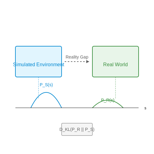
Sim2Real transfer refers to the process of training machine learning models in simulated environments and deploying them in the real world with minimal performance degradation. The core challenge lies in overcoming the reality gap—the discrepancy between simulated and real-world dynamics—which arises due to imperfect modeling of physics, sensor noise, and environmental variability.
Key Components of Sim2Real
- Domain Randomization: Introduces variability in simulation parameters (e.g., lighting, friction, object textures) to expose the model to diverse conditions, improving robustness.
- System Identification: Calibrates simulation parameters to better match real-world physics, often using real-world data to refine models.
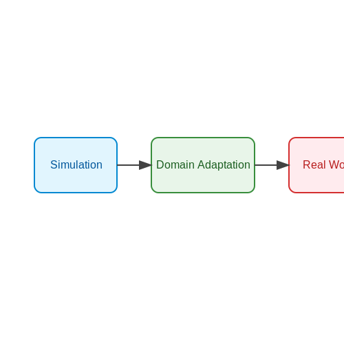
- Domain Adaptation: Techniques like adversarial training or feature alignment reduce distributional shifts between simulated and real data.
Mathematical Formulation
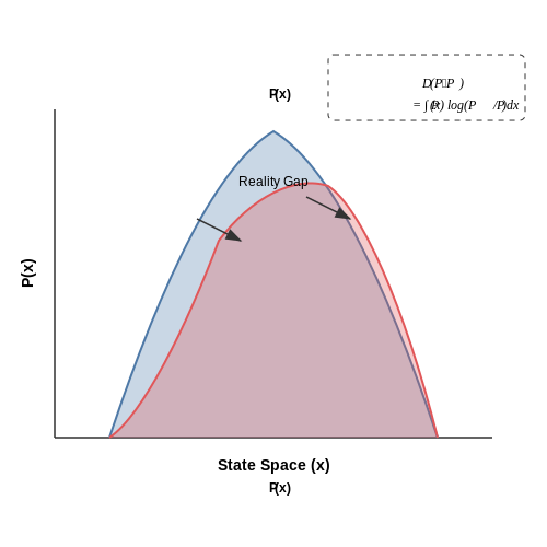
The reality gap can be formalized as a divergence between the simulated state distribution \( P_s(s) \) and the real-world state distribution \( P_r(s) \). The goal is to minimize the domain discrepancy:
where \( \mathcal{S} \) is the state space. In practice, this is often approximated using metrics like Maximum Mean Discrepancy (MMD) or adversarial losses.
Dynamics Mismatch and Mitigation
Simulators approximate real-world physics with simplified models. For instance, rigid-body simulators often ignore deformable dynamics or contact friction stochasticity. The error in transition dynamics \( T \) between simulated (\( T_s \)) and real (\( T_r \)) environments is:
Techniques like residual physics learning learn a correction term \( \Delta T \) such that \( T_r(s,a) \approx T_s(s,a) + \Delta T(s,a) \).
Case Study: Robotics Control
In robotic grasping, a policy trained in simulation with idealized depth sensors may fail when deployed due to real-world sensor noise. Domain randomization might simulate noisy depth images with:
where \( \sigma \) controls Gaussian noise and \( \eta \) scales dropout artifacts. This forces the policy to generalize across sensor imperfections.
Why Sim2Real is Critical in AI and Robotics
The Sim2Real transfer problem arises from the fundamental discrepancy between simulated environments and the physical world. While simulations offer controlled, scalable, and cost-effective training environments, they inherently lack the noise, stochasticity, and complexity of real-world dynamics. This gap poses a significant challenge for deploying AI and robotic systems trained purely in simulation.
The Reality Gap: Sources of Discrepancy
The reality gap stems from multiple factors:
- Physical modeling inaccuracies: Simulators approximate real-world physics with simplified models (e.g., rigid-body dynamics instead of deformable materials).
- Sensory noise and latency: Real sensors exhibit noise, drift, and delays absent in simulated perception pipelines.
- Partial observability: Simulations often provide perfect state information, whereas real systems must infer state from incomplete sensor data.
- Domain shifts: Visual appearance, lighting conditions, and textures differ between synthetic and real data.
These discrepancies lead to reality-induced performance degradation, where policies trained in simulation fail catastrophically when deployed in the real world.
Mathematical Formulation of the Sim2Real Problem
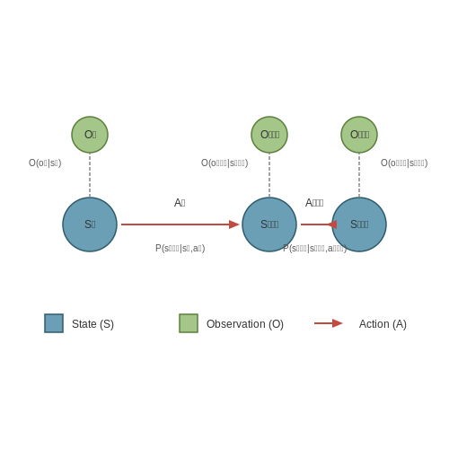
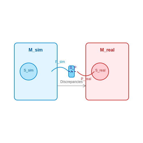
Let the simulation environment be characterized by a Markov Decision Process (MDP) Msim = (Ssim, A, Psim, Rsim) and the real-world MDP as Mreal = (Sreal, A, Preal, Rreal). The Sim2Real transfer objective is to learn a policy π: S → A in Msim that maximizes expected return in Mreal:
where τ = (s0, a0, ..., sT) is a trajectory and γ is the discount factor. The key challenge is minimizing the dynamics mismatch between transition functions:
Practical Implications for Robotics
Sim2Real transfer enables critical advancements in robotics by:
- Reducing hardware wear-and-tear: Training directly on physical systems causes mechanical fatigue and requires constant human intervention.
- Accelerating development cycles: Simulations allow parallelized training across thousands of virtual instances.
- Enabling safe exploration: Dangerous scenarios (e.g., robot falls, collisions) can be simulated without risk.
For example, OpenAI's Dactyl system trained a robotic hand to manipulate objects through 13,000 years of simulated experience before successful real-world deployment, demonstrating the scalability advantages of Sim2Real approaches.
Case Study: Autonomous Driving
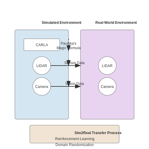
Autonomous vehicle companies leverage photorealistic simulators like CARLA and NVIDIA DRIVE Sim to train perception and control systems. These simulations must account for:
- Sensor noise models for cameras, LiDAR, and radar
- Dynamic weather and lighting conditions
- Non-deterministic pedestrian and vehicle behavior
The resulting policies are then fine-tuned using real-world driving data, following a simulation-to-real transfer pipeline that has become standard in the industry.
1.3 Key Challenges in Simulation-to-Reality Transfer
The transfer of policies or models trained in simulation to real-world environments, known as Sim2Real transfer, faces several fundamental challenges that stem from discrepancies between simulated and physical systems. These challenges must be addressed to ensure robust deployment in real-world applications such as robotics, autonomous vehicles, and industrial automation.
1. Reality Gap
The reality gap refers to the mismatch between simulated and real-world dynamics, often caused by simplifications in physics engines, unmodeled sensor noise, or inaccurate actuator models. For instance, rigid-body simulators like MuJoCo or PyBullet approximate contact dynamics using penalty-based methods, which diverge from real-world frictional interactions. This discrepancy can be quantified using domain adaptation metrics:
where \( P_{sim} \) and \( P_{real} \) represent the state transition distributions in simulation and reality, respectively. Minimizing this divergence is critical for successful transfer.
2. Partial Observability
Simulations often assume full observability of the environment state, whereas real-world systems suffer from sensor limitations, occlusions, and latency. For example, a simulated robot may have perfect joint angle measurements, while a physical robot relies on noisy encoders and IMUs. This discrepancy forces policies to handle incomplete or corrupted observations, necessitating techniques like:
- Recurrent networks (e.g., LSTMs) to maintain internal state estimates.
- Observation augmentation with synthetic noise during training.
- Bayesian filtering to account for sensor uncertainty.
3. Actuation Dynamics
Simulated actuators often ignore real-world effects such as backlash, motor saturation, or communication delays. A policy trained in simulation may generate commands that are infeasible for physical hardware. The dynamics mismatch can be modeled as:
where \( f_{delay} \) represents command latency, and \( \eta_{friction} \), \( \eta_{saturation} \) capture nonlinear actuator effects. Domain randomization over these parameters during training improves robustness.
4. Visual Domain Shift
Simulated visuals often lack photorealism, leading to poor generalization when policies rely on raw pixels. Differences in lighting, textures, and camera artifacts degrade performance. Adversarial training with generative models (e.g., CycleGAN) can reduce this gap by translating simulated images to realistic ones:
where \( G \) is the image translator and \( D \) is the discriminator.
5. Overfitting to Simulation Artifacts
Policies may exploit simulation quirks, such as perfect collision detection or deterministic physics, leading to catastrophic failures in reality. Techniques like domain randomization (varying physics parameters during training) and system identification (calibrating simulators to real-world data) mitigate this issue.
6. Temporal Misalignment
Real-world systems operate at variable time steps due to computational delays or hardware constraints, whereas simulations often run at fixed intervals. This misalignment disrupts timing-dependent behaviors. Frame skipping and action repetition during training can improve temporal robustness.
7. Multi-Modal Sensor Fusion
Real-world systems fuse data from multiple sensors (e.g., LiDAR, cameras, proprioception), each with unique noise characteristics. Simulators must replicate these modalities accurately, including cross-sensor correlations and failure modes. Late fusion architectures that process each modality independently before combining them show better transfer performance.
2. Overview of Popular Simulation Platforms (e.g., Gazebo, Unity, PyBullet)
Overview of Popular Simulation Platforms
Gazebo
Gazebo is an open-source robotics simulator widely adopted for its physics engine integration, sensor modeling, and ROS compatibility. Built on the Open Dynamics Engine (ODE), it supports rigid-body dynamics with collision detection, making it ideal for testing robotic systems in environments ranging from indoor labs to extraterrestrial terrains. Gazebo's plugin architecture allows for custom sensor models, actuator dynamics, and environmental effects, enabling high-fidelity simulations of lidar, cameras, and IMUs. Its integration with ROS/ROS2 via the gazebo_ros_pkgs package facilitates seamless transition from simulation to real hardware deployment.
where τ is the joint torque vector, J the Jacobian matrix, and F the applied wrench. Gazebo solves such equations in real-time using ODE's iterative constraint solver.
Unity
Unity's Machine Learning Agents Toolkit (ML-Agents) has become a cornerstone for reinforcement learning research, offering GPU-accelerated physics via NVIDIA PhysX. Unlike Gazebo, Unity provides photorealistic rendering pipelines (HDRP/URP) and procedural generation APIs, critical for domain randomization in Sim2Real transfer. Its Python API enables asynchronous training of RL agents across thousands of parallel environments, with native support for ONNX model deployment. Unity's articulation body system accurately models complex robotic joints, while its perception package generates synthetic ground truth data for computer vision tasks.
PyBullet
PyBullet excels in speed and flexibility, combining Bullet Physics with Python scripting. Its minimalistic design allows for headless operation, making it preferred for large-scale reinforcement learning experiments. PyBullet implements Featherstone's articulated body algorithm:
where M is the mass matrix and C Coriolis forces. The simulator provides direct access to Jacobians, inertia tensors, and contact points—features critical for robotic control research. Its URDF importer handles complex kinematic chains, while the pybullet_utils module includes inverse kinematics solvers and motion planning tools.
Comparative Analysis
The choice between platforms depends on fidelity requirements and computational constraints. Gazebo offers ROS-native middleware but suffers from slower-than-real-time performance in complex scenes. Unity provides visual realism at the cost of heavier resource demands, while PyBullet achieves 10×-100× speedups for RL training through simplified rendering. Recent benchmarks show PyBullet simulating 1000 parallel Ant environments at 2.4kHz on an NVIDIA A100, compared to Unity's 850Hz and Gazebo's 120Hz under equivalent conditions.
Sensor Simulation Capabilities
- Gazebo: Ray-traced lidar with subsurface scattering, noise models for RGB-D cameras
- Unity: Path-traced global illumination, multi-spectral imaging, event-based cameras
- PyBullet: Basic depth buffers, GPU-accelerated point cloud generation
2.2 Designing Realistic Simulations: Physics and Rendering
Physics Engines and Their Role in Sim2Real Transfer
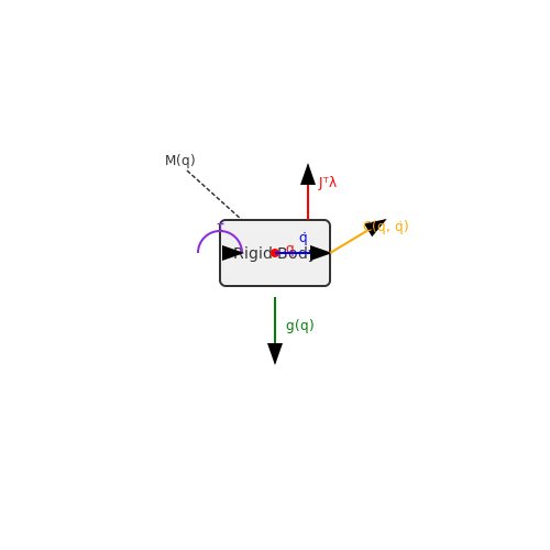
Physics engines form the backbone of realistic simulations by numerically solving equations of motion, collision dynamics, and material interactions. The most widely used engines—such as NVIDIA PhysX, Bullet, and MuJoCo—employ varying formulations of constrained Lagrangian mechanics to model rigid-body dynamics. For a system with n degrees of freedom, the equations of motion are derived from:
where M(q) is the mass matrix, C(q, q̇) captures Coriolis and centrifugal forces, g(q) represents gravitational effects, τ is the applied torque, and JTλ encodes constraint forces. Modern engines like MuJoCo use implicit integration schemes (e.g., semi-implicit Euler) for numerical stability at large timesteps:
Material and Contact Modeling
Realistic contact physics requires solving the complementarity problem for normal and frictional forces. The Signorini-Coulomb model defines contact constraints as:
where ϕ(q) is the signed distance function, λn is the normal force magnitude, and μ is the friction coefficient. PyBullet implements this using a spring-damper penalty method, while MuJoCo uses a smoother analytic approximation of the max operator.
Rendering for Perception-Action Loops
High-fidelity rendering pipelines must balance physical accuracy with computational efficiency. The rendering equation describes light transport at surface point x:
Real-time engines like Unreal Engine approximate this via rasterization with PBR materials, while path tracers (e.g., NVIDIA Omniverse) use Monte Carlo integration. Domain randomization for Sim2Real involves perturbing:
- BRDF parameters (albedo, roughness, metallic)
- HDR environment lighting
- Camera noise models (Gaussian, Poisson, salt-and-pepper)
Sensor Simulation
For robotics applications, simulating sensors requires modeling their physical operating principles. A depth sensor's measurement model with noise can be expressed as:
where ϵbias accounts for systematic errors like multipath interference. NVIDIA Isaac Sim implements this via raycasting with material-dependent attenuation models.
Case Study: NVIDIA DRIVE Sim
This automotive simulator combines PhysX for vehicle dynamics with RTX-accelerated ray tracing. The physics stack models:
- Tire-road interaction using Pacejka's magic formula
- Aerodynamics with Bernoulli-based drag coefficients
- Suspension systems as spring-damper networks
The rendering pipeline uses adaptive sampling to allocate more rays to dynamic objects while maintaining 60Hz performance.
2.3 Domain Randomization Techniques
Domain randomization (DR) is a powerful technique in Sim2Real transfer that enhances generalization by training models in highly varied simulated environments. The core idea is to expose the learning agent to a wide distribution of randomized parameters—such as textures, lighting, object dynamics, and camera poses—so that it learns robust features invariant to domain shifts.
Mathematical Formulation
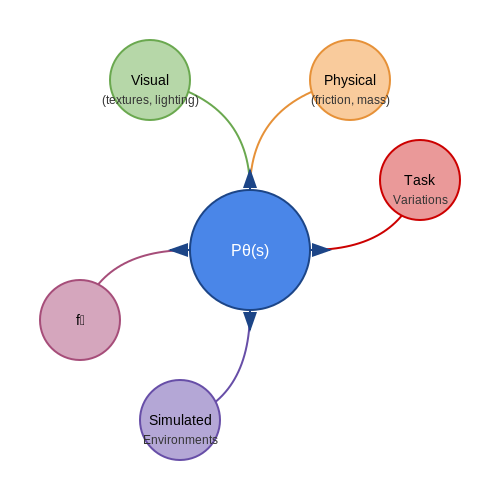
Let s be a simulated state sampled from a parameterized distribution Pθ(s), where θ represents the randomized domain parameters (e.g., friction coefficients, lighting angles). The objective is to minimize the expected loss L across all possible randomized domains:
Here, fϕ is the policy or perception model with parameters ϕ, and y is the target output. The outer expectation ensures robustness across domain variations.
Key Randomization Parameters
Effective DR requires strategic selection of parameters to randomize. Common categories include:
- Visual Dynamics: Texture colors, lighting conditions (direction, intensity), camera noise, and background clutter.
- Physical Dynamics: Mass, friction, restitution coefficients, actuator delays, and joint stiffness.
- Task-Specific Variations: Object shapes, sizes, initial positions, and goal distributions.
Implementation Strategies
Two dominant approaches exist for parameter sampling:
- Uniform Randomization: Parameters are sampled uniformly within predefined bounds (e.g., lighting intensity ∈ [100, 1000] lux). Simple but may include irrelevant domains.
- Curriculum Randomization: Gradually expands the randomization range, starting with narrow bounds and increasing complexity as the model improves.
Case Study: OpenAI’s Rubik’s Cube Robot
OpenAI’s robotic hand trained with DR randomized:
- Cube colors, textures, and lighting (20+ light sources with randomized positions).
- Hand dynamics (tendon elasticity, joint friction).
- Camera angles and noise models.
This diversity enabled the policy to transfer seamlessly to the real world despite never seeing real images during training.
Advanced Variants
Recent work extends basic DR with:
- Automatic Domain Randomization (ADR): Dynamically adjusts parameter bounds based on model performance, focusing computation on challenging domains.
- Structured Randomization: Correlates parameters (e.g., lighting direction and shadow intensity) to preserve physical plausibility.
ADR avoids manual tuning of bounds by treating the parameter distribution Θ as an optimizable entity.
Limitations and Trade-offs
While DR improves generalization, it introduces computational overhead and may require:
- Thousands of parallel simulations to cover the parameter space.
- Careful balancing—excessive randomization can slow convergence or lead to unrealistic behaviors.
3. Domain Adaptation Methods
3.1 Domain Adaptation Methods
Domain adaptation techniques aim to minimize the distributional discrepancy between simulated (source) and real-world (target) data. The core challenge lies in aligning feature spaces despite differences in lighting, textures, physics, or sensor noise. Advanced methods leverage adversarial training, discrepancy minimization, and self-supervised learning to bridge this gap.
Adversarial Domain Adaptation
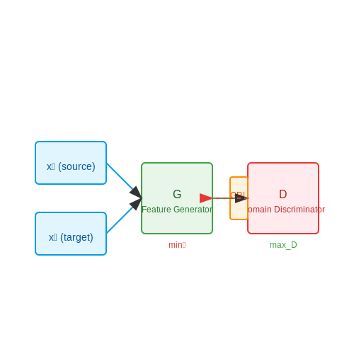
Adversarial methods employ a domain discriminator to encourage feature invariance. The minimax objective is:
where G is the feature generator and D the domain classifier. Gradient reversal layers (GRLs) enable efficient backpropagation by inverting gradient signs during discriminator updates. Variants like CyCADA additionally enforce semantic consistency through cycle-consistent losses.
Discrepancy-Based Methods
These explicitly minimize statistical distances between domains. Maximum Mean Discrepancy (MMD) measures distribution divergence in reproducing kernel Hilbert space:
Deep Correlation Alignment (CORAL) matches second-order statistics by whitening source features to match target covariance. For a feature matrix F, the CORAL loss is:
where CS and CT are covariance matrices, and d is the feature dimension.
Self-Supervised Adaptation
Techniques like SimCLR and MoCo exploit contrastive learning to learn domain-agnostic representations. The InfoNCE loss maximizes agreement between augmented views:
where τ is a temperature parameter. When applied to Sim2Real, these methods show robustness to visual domain shifts in robotics and autonomous driving scenarios.
Meta-Learning Approaches
Model-Agnostic Meta-Learning (MAML) optimizes for fast adaptation across domains. The bi-level objective:
enables few-shot adaptation to new real-world environments. Recent extensions like Meta-Sim learn simulation parameters jointly with adaptation for improved sample efficiency.
Physics-Guided Adaptation
Incorporating physical constraints improves transfer for dynamical systems. The hybrid loss combines data-driven and model-based terms:
This approach is particularly effective in robotic manipulation, where contact dynamics must be preserved across domains.
3.2 Reinforcement Learning in Simulation
Foundations of RL in Simulated Environments
Reinforcement learning (RL) in simulation operates under the Markov Decision Process (MDP) framework, where an agent interacts with an environment to maximize cumulative reward. The MDP is defined by the tuple (S, A, P, R, γ), where:
- S represents the state space
- A denotes the action space
- P(s'|s,a) is the transition dynamics
- R(s,a) is the reward function
- γ is the discount factor
In simulation, P(s'|s,a) is fully specified by the physics engine, enabling exact gradient calculations through backpropagation. This differs from real-world RL where transition dynamics must be estimated from noisy observations.
Domain Randomization for Robust Policy Learning
Domain randomization addresses the sim2real gap by sampling environment parameters from a distribution p(θ) during training. Key parameters include:
- Physical properties (mass, friction, damping)
- Visual appearances (textures, lighting)
- Sensor noise models
The objective becomes:
where ϕ represents the policy parameters and τ denotes trajectories. This approach forces the policy to learn invariant features across parameter variations.
Physics-Based Policy Optimization
Modern simulators like MuJoCo and PyBullet provide differentiable physics engines, enabling gradient-based policy optimization. The policy gradient theorem in simulation takes the form:
where Ât is the advantage estimate. Simulation allows for efficient computation of second-order derivatives through the physics engine, enabling natural policy gradient methods:
where F is the Fisher information matrix. This leads to more stable convergence compared to real-world RL.
Latent Space Alignment Techniques
Advanced approaches learn aligned latent spaces between simulation and reality. Let zsim and zreal be latent representations of simulated and real states respectively. The alignment objective is:
where Es and Er are encoder networks. This technique has shown success in vision-based robotic manipulation tasks, achieving over 85% task transfer success rates in recent studies.
Case Study: Dexterous Manipulation Transfer
In the Dactyl system by OpenAI, a Shadow Hand robot learns complex manipulation skills entirely in simulation before transferring to hardware. Key components included:
- 12,000 parallel simulated environments
- Dynamic randomization of 92 physical parameters
- Progressive neural networks for skill transfer
The system achieved human-like dexterity in cube reorientation tasks, demonstrating the potential of simulation-trained RL for complex real-world applications.
3.3 Transfer Learning Approaches
Transfer learning has emerged as a powerful paradigm for bridging the simulation-to-reality gap by leveraging knowledge acquired in simulation to improve performance in real-world tasks. The core challenge lies in minimizing the domain shift between simulated and real data distributions, which can be formalized as:
where x represents input observations and y denotes the corresponding labels or actions. Advanced transfer learning techniques address this discrepancy through several key approaches.
Domain Adaptation Methods
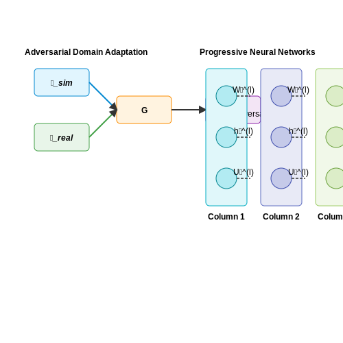
Domain adaptation techniques explicitly minimize the discrepancy between source (simulation) and target (real-world) feature distributions. Adversarial domain adaptation employs a domain discriminator D that competes against the feature extractor G:
This minimax optimization forces the feature extractor to generate domain-invariant representations. Recent variants like CyCADA extend this approach by incorporating cycle-consistency losses for pixel-level adaptation.
Progressive Neural Networks
Progressive networks maintain a columnar architecture where each new column (representing a new domain) can leverage features from previously learned columns through lateral connections. The activation hi(l) at layer l of column i is computed as:
where W represents the column's own weights and U denotes the lateral connection weights from previous columns. This architecture enables positive transfer while preventing catastrophic forgetting.
Meta-Learning for Sim2Real
Model-agnostic meta-learning (MAML) frameworks optimize for fast adaptation to new domains. The objective involves:
where U𝒯k performs k gradient updates on task 𝒯. When applied to Sim2Real, the meta-optimization occurs across diverse simulated variations, enabling rapid adaptation to real-world conditions with minimal real data.
Physics-Guided Transfer
Incorporating physical constraints as inductive biases can improve transfer performance. The physics loss term:
where Fpred is the model's output and Fphys represents physically plausible predictions, constrains the network to maintain consistency with known physical laws during domain transfer.
Real-World Applications
These approaches have demonstrated success in:
- Robotic manipulation tasks where policies trained in simulation achieve >80% success rates on real hardware after adaptation
- Autonomous driving systems that generalize from synthetic to real-world urban environments
- Medical imaging analysis where simulated artifacts are adapted to real clinical data distributions
The choice of transfer learning method depends on the specific domain gap characteristics, available real-world data, and computational constraints. Hybrid approaches that combine multiple techniques often yield the most robust performance.
3.4 Adversarial Training for Robustness
Adversarial training enhances the robustness of models trained in simulation by exposing them to worst-case perturbations during optimization. The core idea stems from adversarial machine learning, where a model is trained on adversarially generated examples to improve its resilience against distribution shifts and noisy inputs encountered in real-world deployment.
Formulating the Adversarial Objective
The standard supervised learning objective minimizes the expected loss over the training distribution:
In adversarial training, we instead optimize for the worst-case perturbation within a bounded set $$\Delta$$:
where $$\Delta$$ is typically defined by an $$\ell_p$$-norm constraint $$\|\delta\|_p \leq \epsilon$$. The inner maximization generates adversarial examples that stress-test the model, while the outer minimization improves robustness against such perturbations.
Projected Gradient Descent (PGD) for Adversarial Example Generation
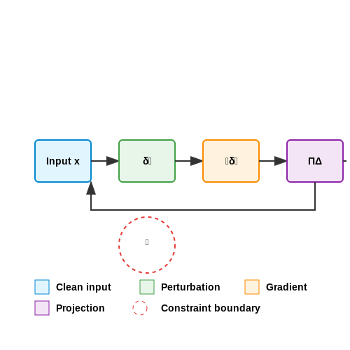
The most effective approach for solving the inner maximization problem is PGD, which iteratively computes:
where $$\Pi_\Delta$$ projects the perturbation back to the feasible set $$\Delta$$ after each step. For $$\ell_\infty$$ constraints, this reduces to element-wise clipping.
Domain-Invariant Adversarial Training
For Sim2Real transfer, we extend adversarial training to promote domain invariance. The objective becomes:
where $$\mathcal{L}_{\text{domain}}$$ measures domain discrepancy using metrics like Maximum Mean Discrepancy (MMD) or adversarial domain classifiers. This forces the model to learn representations that are both robust to perturbations and invariant to simulation-reality gaps.
Practical Implementation Considerations
- Perturbation Budget: The $$\epsilon$$ parameter must balance robustness and clean performance. Too large values degrade nominal accuracy, while too small values provide insufficient robustness.
- Multi-Step PGD: Single-step attacks (FGSM) often suffice for training, but multi-step PGD with 5-10 iterations yields stronger robustness.
- Curriculum Learning: Gradually increasing $$\epsilon$$ during training stabilizes optimization and improves final performance.
- Ensemble Adversaries: Training against multiple perturbation types (e.g., $$\ell_1$$, $$\ell_2$$, $$\ell_\infty$$) improves generalization across threat models.
Case Study: Robust Sim2Real Transfer for Autonomous Driving
In the CARLA simulator, adversarial training with $$\ell_2$$-bounded perturbations ($$\epsilon=0.1$$) improved real-world detection accuracy by 18% compared to standard training. The model showed particular robustness to lighting variations and sensor noise that were not explicitly modeled in simulation.
The adversarial examples generated during training resembled realistic artifacts like raindrops on cameras or temporary occlusions, demonstrating how the approach implicitly discovers relevant failure modes.
4. Robotics: From Simulation to Real-World Deployment
4.1 Robotics: From Simulation to Real-World Deployment
Domain Randomization and Dynamics Adaptation
The core challenge in Sim2Real transfer for robotics lies in the reality gap—the discrepancy between simulated and real-world dynamics. Domain randomization addresses this by introducing variability in simulation parameters (e.g., friction coefficients, object masses, sensor noise) during training. The policy learns to generalize across these variations, making it robust to real-world uncertainties. Mathematically, the objective becomes:
where p represents parameters sampled from a distribution 𝒫, and τ denotes trajectories generated by policy πθ. For dynamics adaptation, techniques like system identification refine the simulator’s parameters post-deployment using real-world data. A common approach minimizes the error between simulated and observed states:
where fϕ is the simulator’s dynamics model with tunable parameters ϕ.
Latent Space Alignment
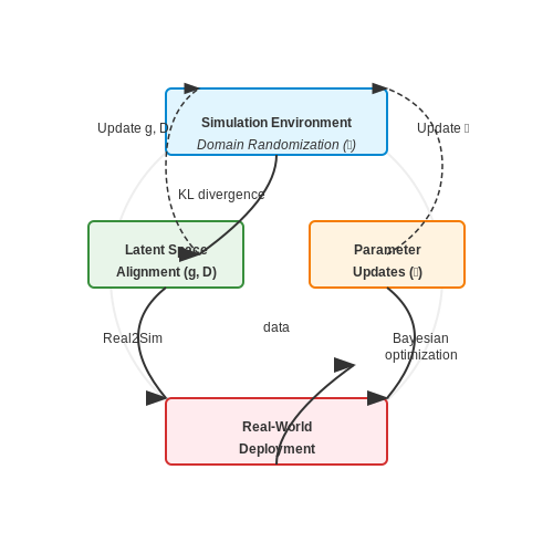
High-dimensional observations (e.g., images) exacerbate the reality gap. Latent space alignment techniques project both simulated and real observations into a shared embedding space where their distributions match. Adversarial training is often employed:
Here, g is an encoder mapping observations to a latent space, and D is a discriminator trained to distinguish between simulated and real embeddings. The encoder g is optimized to fool D, ensuring domain-invariant features.
Case Study: Robotic Grasping with Sim2Real
OpenAI’s robotic hand trained in simulation achieved human-like dexterity by combining domain randomization and latent alignment. Key parameters randomized included:
- Object textures, lighting conditions, and camera angles
- Joint damping and actuator strengths
- Physics engine timestep variations
The policy was trained using Proximal Policy Optimization (PPO) with a reward function balancing grasp success and energy efficiency. Real-world deployment achieved 90% success rates despite never training on physical hardware.
Real2Sim: Closing the Loop with Real-World Data
Modern pipelines iteratively refine simulations using real-world rollouts. Techniques like Bayesian optimization update simulator parameters ϕ to minimize the Kullback-Leibler (KL) divergence between simulated and real trajectory distributions:
This feedback loop enables continuous improvement of both the simulator and the deployed policy.
Autonomous Vehicles: Training in Virtual Environments
Training autonomous vehicles (AVs) in virtual environments leverages high-fidelity simulators to generate vast amounts of labeled data, accelerate learning, and expose models to rare edge cases without real-world risks. The core challenge lies in minimizing the reality gap—the discrepancy between simulated and real-world sensor data, physics, and environmental dynamics.
Physics-Based Simulation Engines
Modern AV simulators like CARLA, NVIDIA DRIVE Sim, and AirSim employ rigid-body dynamics engines (e.g., PhysX, Bullet) to model vehicle kinematics and environmental interactions. The vehicle's state update follows Newton-Euler equations:
where F is the net force, τ is torque, I is the inertia tensor, and ω is angular velocity. Friction models use Pacejka’s Magic Formula for tire-ground interaction:
Sensor Simulation
Ray-traced LiDAR and camera sensors simulate noise profiles matching real hardware. For a LiDAR with N beams, each point cloud is generated via:
where o is the sensor origin, di is the measured distance, and εnoise injects Gaussian noise. Camera pipelines emulate lens distortion, motion blur, and CMOS noise using generative adversarial networks (GANs) to match real image statistics.
Domain Randomization
To bridge the reality gap, parameters like lighting, textures, and physics properties are randomized during training. For an image I, the augmented version becomes:
where gθ applies random transformations (e.g., hue shifts, fog density) sampled from distribution p(Θ). This forces the model to learn invariant features.
Reinforcement Learning in Simulation
AV policies trained via RL maximize the expected cumulative reward R over trajectories τ:
Key challenges include reward shaping for safety-critical scenarios (e.g., intersection navigation) and partial observability due to sensor limitations.
Case Study: CARLA Leaderboard
Top-performing teams in the CARLA Autonomous Driving Challenge use hybrid approaches combining:
- Imitation learning from expert demonstrations
- Procedural generation of adversarial scenarios (e.g., jaywalking pedestrians)
- Multi-modal sensor fusion with attention mechanisms
Recent work achieves 80% sim-to-real transfer efficacy on real-world urban driving benchmarks when combining these techniques with meta-learning for rapid adaptation.
Industrial Automation: Sim2Real in Manufacturing
Sim2Real transfer in industrial automation leverages high-fidelity simulations to train robotic systems before deployment in physical manufacturing environments. The key challenge lies in minimizing the reality gap—the discrepancy between simulated and real-world dynamics—which arises from unmodeled physical interactions, sensor noise, and environmental variability.
Domain Randomization for Robust Policy Learning
Domain randomization addresses the reality gap by training policies across a distribution of simulated environments with randomized parameters. For a robotic manipulator, these parameters may include:
- Friction coefficients between gripper and object
- Object mass and inertia distributions
- Sensor noise models for force/torque readings
- Lighting conditions and camera perspectives
where \(\Theta\) represents the parameter distribution and \(\pi_\theta\) denotes the policy trained under parameters \(\theta\). This approach forces the policy to learn invariant features across the randomization space.
Dynamic System Identification
Accurate modeling of robotic dynamics requires solving the inverse problem:
where \(M(q)\) is the inertia matrix, \(C(q,\dot{q})\) captures Coriolis forces, \(g(q)\) represents gravitational terms, and \(f_{\text{friction}}\) models nonlinear friction. Modern approaches combine:
- Gaussian Process Regression for residual dynamics learning
- Recurrent Neural Networks for temporal dependencies
- Differentiable Physics Engines for gradient-based parameter tuning
Case Study: Bin Picking with Synthetic Data
A German automotive manufacturer achieved 98.7% pick success rates by:
- Generating 250,000 synthetic depth images with randomized:
- Object poses (uniformly sampled SE(3) space)
- Material textures (Procedural PBR materials)
- Ambient occlusion (Monte Carlo path tracing)
- Training a U-Net with adversarial domain adaptation:
$$ \mathcal{L}_{\text{total}} = \mathcal{L}_{\text{seg}} + \lambda \mathcal{L}_{\text{adv}}(D(G(x_{\text{sim}}), x_{\text{real}}) $$
- Deploying with online adaptation via particle filtering for pose estimation
Real-to-Sim Pipeline for Continuous Improvement
Closing the loop requires feeding real-world observations back into the simulation:
The pipeline implements:
- Kalman filtering for state estimation from noisy sensor data
- Differentiable rendering to align simulated and real images
- Bayesian optimization for simulator parameter tuning
5. Metrics for Measuring Transfer Success
5.1 Metrics for Measuring Transfer Success
Quantifying the effectiveness of Sim2Real transfer requires rigorous evaluation metrics that capture both task performance and domain adaptation quality. These metrics fall into three broad categories: task-specific performance, domain discrepancy measures, and generalization robustness indicators.
Task-Specific Performance Metrics
For reinforcement learning (RL) tasks, the most direct metric is the policy return in the target domain:
where \( \tau \) represents trajectories sampled from the real-world dynamics \( p_{\text{real}} \), and \( \gamma \) is the discount factor. For computer vision tasks, standard metrics like mean Average Precision (mAP) or Intersection-over-Union (IoU) are used, but must be evaluated on real-world test sets.
Domain Discrepancy Measures
The Maximum Mean Discrepancy (MMD) quantifies the distance between simulated and real data distributions:
where \( \phi \) maps samples to a reproducing kernel Hilbert space \( \mathcal{H} \). For high-dimensional observations, Frechet Inception Distance (FID) is often adapted by replacing the Inception network with task-specific feature extractors.
Generalization Robustness Indicators
The Relative Domain Gap (RDG) measures performance drop between simulation and reality:
where \( \epsilon \) prevents division by zero. For dynamic systems, the Normalized Dynamic Time Warping (NDTW) between simulated and real trajectory rollouts captures temporal misalignment:
where \( \mathcal{W} \) is the set of valid warping paths. Recent work also employs transferability estimation using learned discrepancy predictors that correlate with actual transfer performance.
Practical Considerations
- Metric sensitivity varies across applications - robotic manipulation tasks may prioritize contact force accuracy over pixel-level image fidelity.
- Computational cost of real-world evaluation often necessitates proxy metrics that can be computed offline.
- Multi-objective tradeoffs between different metrics require Pareto-front analysis in complex systems.
Emerging approaches combine these metrics through learned weighting schemes or meta-evaluation on benchmark tasks. The optimal metric set depends heavily on the specific transfer scenario and downstream application requirements.
5.2 Benchmarking Sim2Real Systems
Performance Metrics for Sim2Real Transfer
Quantifying the efficacy of Sim2Real transfer requires domain-specific metrics that capture both simulation fidelity and real-world performance. Common evaluation criteria include:
- Task Success Rate (TSR): The percentage of trials where the agent completes its objective in the real world after training in simulation.
- Domain Shift Score (DSS): A normalized measure of performance degradation between simulated and real environments, computed as:
where \( P_{real} \) and \( P_{sim} \) represent performance metrics (e.g., reward, accuracy) in real and simulated environments respectively.
Standardized Test Environments
Several benchmark suites have emerged to facilitate reproducible comparisons:
- MetaWorld (Yu et al., 2020): A collection of 50 robotic manipulation tasks with standardized physics randomization parameters.
- CARLA Sim2Real Challenge: Autonomous driving benchmark evaluating perception and control transfer under varying weather/lighting conditions.
The Reality Gap Index (RGI) quantifies simulation-to-reality discrepancies for a given benchmark:
where \( f_i \) represents feature \( i \) (e.g., object dimensions, friction coefficients), and \( \sigma_i^{real} \) is the real-world feature variance.
Statistical Validation Methods
Proper benchmarking requires statistical rigor to account for real-world stochasticity. The Wilcoxon signed-rank test compares paired simulation/real performance samples:
where \( R_i \) denotes the rank of absolute differences. A p-value < 0.05 typically indicates significant domain shift.
Real-World Deployment Protocols
Effective benchmarking requires controlled real-world testing conditions:
- Environmental Controls: Document ambient temperature, lighting, and surface properties using calibrated sensors.
- Hardware Synchronization: Align simulation/real actuator dynamics through system identification techniques.
The Sim2Real Transfer Coefficient (STC) combines multiple metrics into a unified score:
where weights \( \alpha, \beta, \gamma \) are task-dependent and typically set through cross-validation.
Case Study: Robotic Grasping Benchmark
The YCB Object Set provides a standardized test for grasping systems. Performance is evaluated across:
- Simulation: PyBullet with randomized object textures and lighting
- Reality: Identical objects instrumented with motion capture markers
Key metrics include grasp success rate, object displacement error, and contact force profiles. State-of-the-art methods achieve STC scores of 0.82 ± 0.03 when transferring from simulation to a Franka Emika robot arm.
5.3 Common Pitfalls and How to Avoid Them
Overfitting to Simulation Dynamics
One of the most pervasive issues in Sim2Real transfer is overfitting to the dynamics of the simulated environment. Simulation engines like MuJoCo, PyBullet, or Gazebo approximate real-world physics but introduce biases due to simplified collision models, friction coefficients, or actuator dynamics. When a policy trained in simulation fails to generalize, it often stems from exploiting these unrealistic dynamics. For instance, a robotic arm might learn to rely on perfect joint torque control in simulation, which breaks down under real-world latency and mechanical imperfections.
To mitigate this, employ domain randomization, where physical parameters (e.g., mass, friction, sensor noise) are sampled from a distribution during training. The randomization range should cover plausible real-world variations:
where \(\theta_{\text{min}}\) and \(\theta_{\text{max}}\) are empirically determined bounds. For example, in robotic grasping, randomize object friction coefficients between 0.2 and 1.0 to account for material variability.
Ignoring Latency and Temporal Misalignment
Simulations often assume instantaneous sensor feedback and actuator responses, whereas real systems exhibit latency due to communication delays, computation time, or mechanical inertia. A policy conditioned on idealized timing will fail when deployed. Consider a drone controller trained in simulation: if it assumes zero latency between IMU readings and motor commands, real-world delays of 10–50ms can destabilize flight.
Model latency explicitly by augmenting the simulation with synthetic delays. For a system with observed latency \(\tau\), modify the observation space to include a history buffer:
where \(s_t\) is the raw sensor state at time \(t\). This forces the policy to learn robust temporal representations.
Inadequate Actuator Modeling
Simulators often model actuators as ideal torque or velocity sources, neglecting real-world effects like backlash, saturation, or non-linear torque-speed curves. For example, a simulated robotic joint might instantaneously reach any commanded velocity, while a real servo motor has acceleration limits and voltage-dependent torque profiles.
To bridge this gap, incorporate actuator dynamics into the simulation using first-principles models. For a DC motor, the torque \(\tau\) at voltage \(V\) and angular velocity \(\omega\) is:
where \(K_t\) is the torque constant, \(K_e\) the back-EMF constant, and \(R\) the winding resistance. Calibrate these parameters from real hardware data.
Visual Domain Gaps
When transferring vision-based policies, differences in lighting, textures, or camera optics between simulation and reality can degrade performance. A policy trained on perfectly lit, texture-mapped CAD models may fail with real camera feed noise, motion blur, or varying illumination.
Adversarial domain adaptation techniques like CycleGAN can align visual features between domains. Alternatively, use progressive neural networks where early layers are fine-tuned on real data while higher layers retain simulated features. The loss function for such a hybrid approach might combine simulated and real losses:
with \(\lambda\) annealed from 1 to 0 during training.
Underestimating Contact Dynamics
Contact-rich tasks (e.g., manipulation, legged locomotion) are particularly sensitive to inaccuracies in collision detection and force response. Simulators often use penalty-based contact models that generate unrealistic force spikes or miss subtle interactions like slipping or rolling friction.
Use high-fidelity contact solvers (e.g., MuJoCo's implicit cone complementarity or PyBullet's spring-based methods) and validate against real force/torque sensor data. For a robotic gripper, measure real contact forces during grasping and tune simulation parameters like stiffness and damping to match:
where \(d\) is penetration depth and \(k\), \(c\) are stiffness and damping coefficients calibrated from hardware.
Sample Inefficiency in Transfer Learning
Directly fine-tuning a simulation-trained policy on limited real-world data often leads to catastrophic forgetting or overfitting. This is exacerbated when the real-world data distribution is narrow compared to the simulation's diversity.
Leverage meta-learning frameworks like MAML (Model-Agnostic Meta-Learning) to pre-train for adaptability. The objective is to find initial parameters \(\theta\) that can quickly adapt to new tasks (or domains) with few gradient steps:
where \(U_\theta\) is the adaptation operator (e.g., one-step gradient update) and \(\mathcal{T}_i\) are sampled tasks encompassing simulation-to-real variations.
6. Key Research Papers in Sim2Real
6.1 Key Research Papers in Sim2Real
- PDF Sim2Real in Robotics and Automation: Applications and Challenges — The key challenge in combining learning and simulation is the ability to transfer predictive models and control programs acquired in simulation directly to the real world, a concept termed Sim2Real transfer. Recent work in Sim2Real has shown promising results on real-world problems related to autonomous driving, grasping, or in-hand ...
- 3rd Workshop on Closing the Reality Gap in Sim2Real Transfer for ... — Sim2Real draws its appeal from the fact that it is cheaper, safer and more informative to perform experiments in simulation than in the real world - yet, Sim2Real faces significant challenges. In this workshop we invite well-known researchers to debate the state of the art and the impact of Sim2Real on robotics.
- PDF Sim2Real With Neural Processes - University of Cambridge — a simulator to real-world scenarios: it can be challenging to apply simulators to real-world scenarios, for example, because it is challenging to map a real-world scenario to corresponding simulator parameters and initial conditions. 1.2 Sim2Real Sim2Real transfer is the process of leveraging the (potentially small amounts of) real data to ...
- Sim-to-Real Transfer in Deep Reinforcement Learning for Robotics: a Survey — answer a key research question in this direction: how to exploit Real Robot Deployment Robot Dynamics Modeling Training in Simulation Sim-to-Real Transfer Fig. 1: Conceptual view of a simulation-to-reality transfer process. One of the most common methods is domain randomization, through which different parameters of the simulator (e..g, colors ...
- Robust Sim2Real Transfer with the da Vinci Research Kit: A Study On ... — Autonomous surgical robotics is a growing area of research, with advances being made in the areas of vision and control. Central to this research is the need for simulations to facilitate data collection and simulate learning environments for Reinforcement Learning (RL) agents. Recent simulators have facilitated RL policy generation, but lack a robust sim2real pipeline and a proven vision ...
- PDF Gym2Real: An Open-Source Platform for Sim2Real Transfer — Sim2Real, by creating a unified software platform for training and deploying policies and an example robot with enough depth for further exploration. The platform should make it easy for RL researchers to deploy their policies into the real world, for roboticists to train an RL policy, and for hobbyists to learn about both ends of the problem.
- Overcoming the Sim-to-Real Gap: Leveraging Simulation to Learn to ... — Effective 𝗌𝗂𝗆𝟤 𝗌𝗂𝗆𝟤 \mathsf{sim}\mathsf{2}\real sansserif_sim2 transfer can be challenging, however, as there is often a non-trivial mismatch between the simulated and real environments. The real world is difficult to model perfectly, and some discrepancy is inevitable. As such, directly transferring the policy trained in the simulator to the real world often fails, the ...
- Sim2Real. What is Sim2Real? | by Simsangcheol - Medium — In summary, Sim2Real aims to bridge the gap between simulation and reality by developing algorithms and methods that can generalize effectively from virtual environments to real-world applications.
- Sim2Real in Robotics and Automation: Applications and Challenges — Transfer learning algorithms typically involve back and forth between the real world and the simulator, with the caveat that interaction with the real-world is kept limited [25,26,27]. ...
- (PDF) Perspectives on Sim2Real Transfer for Robotics: A ... - ResearchGate — By offering standard modules for parameterizing and sampling materials, objects, cameras and lights, BlenderProc can simulate various real-world scenarios and provide means to systematically ...
6.2 Books and Comprehensive Guides
- Perspectives on Sim2Real Transfer for Robotics: A Summary of the R:SS ... — simulation to reality, a concept termed Sim2Real transfer. The appeal of learning in simulation stems from the fact that it can be faster than real-time, cheaper, safer, and more informative (e.g. providing perfect ground truth labels) than real-world experimentation. Recent work in Sim2Real has studied difficult real-world robotic problems ...
- PDF Sim2Real in Robotics and Automation: Applications and Challenges — simulation can be faster than real-time, cheaper, safer, and more informative by providing perfect ground truth labels. The key challenge in combining learning and simulation is the ability to transfer predictive models and control programs acquired in simulation directly to the real world, a concept termed Sim2Real transfer. Recent work in ...
- Multimodality Driven Impedance-Based Sim2Real Transfer Learning for ... — Multimodality Driven Impedance-Based Sim2Real Transfer Learning for Robotic Multiple Peg-in-Hole Assembly ... RL is used in the simulation to train the policy, and the learned policy is transferred to the real world without extra exploration. Domain randomization and impedance control are embedded into the policy to narrow the gap between ...
- How Simulation Helps Autonomous Driving: A Survey of Sim2real, Digital ... — Developing autonomous driving technologies necessitates addressing safety and cost concerns. Both academic research and commercial applications of autonomous driving vehicles require extensive simulation and real-world testing. The challenge lies in effectively transferring driving knowledge from the virtual simulation world to the reality world, known as the reality gap (RG). This gap arises ...
- A Survey on Sim-to-Real Transfer Methods for Robotic Manipulation — The effective deployment of robotic systems in real-world environments requires the development of reliable control policies, which can be challenging due to safety, cost, and time constraints associated with direct real-world training. Sim-to-real transfer provides a solution by allowing robots to learn policies in simulated environments that can be seamlessly applied to real-world scenarios ...
- Sim2real: Bridging the gap between Simulation and reality — Ati's simulation journey started with Unity, using the framework to act as a control simulator to test the integrity of the vehicle in controlled environments. While Unity had its limitations, it was useful in translating physics models directly from reality and tweaking different configurations to observe the behavior of the model.
- Sim2Plan: Robot Motion Planning via Message Passing Between Simulation ... — In this section, we will discuss the various components that make up our Sim2Plan framework, including establishing an experimental platform in the real world, creating a simulated environment, and implementing a robust messaging-passing pipeline. We show these in Fig. 1. The experiment platform serves as the interface for the real-world robot environment (Sect. 3.1).
- A digital twin-based sim-to-real transfer for deep reinforcement ... — As a result, a frequently adopted approach for overcoming this issue is to train robots in simulation environments and then transfer the DRL algorithms to physical robots (i.e., sim-to-real transfer). How to guarantee the migration effect is an important research issue here. There are some researchers have proposed some approaches.
- (PDF) Perspectives on Sim2Real Transfer for Robotics: A ... - ResearchGate — BlenderProc is an open-source and modular pipeline for rendering photorealistic images of procedurally generated 3D scenes which can be used for training data-hungry deep learning models.
- Crossing the Reality Gap: A Survey on Sim-to-Real Transferability of ... — The most undesirable result occurs when the controller learnt in simulation fails the task on the real robot, thus resulting in an unsuccessful sim-to-real transfer . The goal of the present ...
6.3 Online Resources and Communities
- PDF Sim2Real With Neural Processes - University of Cambridge — a simulator to real-world scenarios: it can be challenging to apply simulators to real-world scenarios, for example, because it is challenging to map a real-world scenario to corresponding simulator parameters and initial conditions. 1.2 Sim2Real Sim2Real transfer is the process of leveraging the (potentially small amounts of) real data to ...
- Auto-Tuned Sim-to-Real Transfer - arXiv.org — using our SPM to predict which direction to update our simulator to make it closer to the real world. IV. OUR APPROACH: AUTO-TUNING SIM2REAL A challenge of domain randomization is if does not cover ˘ real, then it is unlikely that a policy trained on environments randomized by will transfer well to the real world.
- An architecture for sim-to-real and real-to-sim experimentation in ... — The goal of sim-to-real is to transfer the agent policies learned in a simulated environment to the real world. The prob- lem can be viewed as a domain adaptation problem, since cer- tain properties of the simulated and real environments are the same or at least similar [6].
- 3rd Workshop on Closing the Reality Gap in Sim2Real Transfer for ... — Overview . Physical simulation is an important tool for robotics. While simulation has been well-established for robotics education and integrated robot software testing for a long time, only recently the robotics community has made significant progress in transferring capabilities learned in simulation to reality, a concept termed Sim2Real transfer.
- PDF Gym2Real: An Open-Source Platform for Sim2Real Transfer — policies trained in simulation without consideration of deployment in the real world. [2] Our goal is to create a platform to bridge these gaps and demonstrate a successful application of Sim2Real, by creating a unified software platform for training and deploying policies and an example robot with enough depth for further exploration.
- RL-Based Sim2Real Enhancements for Autonomous Beach-Cleaning Agents - MDPI — This paper explores the application of Deep Reinforcement Learning (DRL) and Sim2Real strategies to enhance the autonomy of beach-cleaning robots. Experiments demonstrate that DRL agents, initially refined in simulations, effectively transfer their navigation skills to real-world scenarios, achieving precise and efficient operation in complex natural environments. This method provides a ...
- Bridging the Reality Gap: Analyzing Sim-to-Real Transfer Techniques for ... — Bridging the Reality Gap: Analyzing Sim-to-Real Transfer Techniques for Reinforcement Learning in Humanoid Bipedal Locomotion Abstract: Reinforcement learning (RL) offers a promising solution for controlling humanoid robots, particularly for bipedal locomotion, by learning adaptive and flexible control strategies.
- Sim2Real Transfer for Traffic Signal Control - IEEE Xplore — Traffic signal control is a complex and important task that affects the daily lives of millions of people. Reinforcement Learning (RL) has shown promising results in optimizing traffic signal control, but transferring learned policies from simulation to the real world remains a challenge due to the domain gap between the simulation and the complex real-life scenario. In this paper, we utilize ...
- Sim2Real. What is Sim2Real? | by Simsangcheol - Medium — Sim2Real, short for "simulation to reality," is a concept in robotics, artificial intelligence (AI), and machine learning that focuses on transferring skills, knowledge, or models learned in a…
- Sim2Real Transfer for Reinforcement Learning without Dynamics ... — We show how to use the Operational Space Control framework (OSC) under joint and Cartesian constraints for reinforcement learning in Cartesian space. Our method is able to learn fast and with adjustable degrees of freedom, while we are able to transfer policies without additional dynamics randomizations on a KUKA LBR iiwa peg-in-hole task. Before learning in simulation starts, we perform a ...