Federated LLM Training Across Edge Devices
1. Core Principles of Federated Learning
Core Principles of Federated Learning
Federated learning (FL) is a decentralized machine learning paradigm where model training occurs across multiple edge devices or nodes without centralized data aggregation. The core objective is to learn a global model while keeping raw data localized, addressing privacy, bandwidth, and latency constraints inherent in traditional centralized approaches.
Mathematical Formulation
The standard FL optimization problem minimizes a global objective function F(w) across K participating devices:
where w represents the model parameters, pk is the weight of the k-th device (typically proportional to its data volume), and Fk(w) is the local objective for device k. The local objective is often the empirical risk over the device's data distribution Dk:
Key Architectural Components
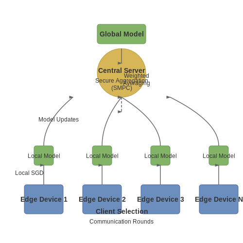
- Client Selection: A subset of devices is sampled each round based on system constraints (battery, connectivity) and statistical requirements.
- Local Training: Each selected device computes a model update using its local data, typically via stochastic gradient descent (SGD):
- Secure Aggregation: Updates are transmitted to a central server through cryptographic protocols like secure multi-party computation (SMPC) or differential privacy mechanisms.
- Model Fusion: The server aggregates updates (e.g., via weighted averaging) to produce a new global model:
Convergence Guarantees
Under convexity and smoothness assumptions, federated SGD achieves convergence at rate O(1/√T) for non-IID data distributions, where T is the number of communication rounds. The convergence bound depends critically on:
- Data heterogeneity (measured via gradient dissimilarity)
- Device participation frequency
- Local computation-to-communication ratio
Practical Challenges
Real-world FL systems must address:
- System Heterogeneity: Variability in device hardware, network conditions, and availability.
- Statistical Heterogeneity: Non-IID data distributions across devices.
- Privacy-Accuracy Tradeoffs: Stronger privacy guarantees (e.g., differential privacy) typically degrade model performance.
Challenges in Scaling LLMs to Edge Devices
Computational Constraints
Edge devices typically operate with limited computational resources compared to cloud servers. Training large language models (LLMs) requires significant floating-point operations (FLOPs), often exceeding the capabilities of edge hardware. For instance, a single forward pass of GPT-3 with 175 billion parameters demands approximately:
where N is the sequence length, dmodel is the model dimension, and L is the number of layers. This computational intensity makes real-time inference challenging on edge devices with constrained CPUs or GPUs.
Memory Limitations
LLMs require substantial memory for both model parameters and intermediate activations. The memory footprint M of a model can be approximated by:
where P represents the number of parameters (in bytes) and A accounts for activation memory. For a 1-billion parameter model with 16-bit precision, this exceeds 2GB—often surpassing the RAM available on edge devices.
Energy Efficiency
Edge devices operate under strict power budgets. The energy consumption E of matrix multiplications—the core operation in transformers—scales cubically with dimension:
where n is the matrix dimension. This creates thermal and battery life challenges for mobile deployment.
Communication Bottlenecks
Federated learning introduces communication overhead between edge devices and aggregators. The required bandwidth B grows with model size S and update frequency f:
For large models, this can saturate wireless networks and incur latency penalties.
Heterogeneous Hardware
Edge ecosystems contain diverse processors (CPUs, GPUs, TPUs, NPUs) with varying:
- Instruction set architectures (ARM vs x86)
- Memory hierarchies (shared vs distributed)
- Numerical precision support (FP32, FP16, INT8)
This heterogeneity complicates optimization and requires specialized compilation techniques like quantization-aware training.
Privacy-Preserving Constraints
Federated learning must maintain privacy while training on sensitive edge data. Techniques like differential privacy add noise η to gradients:
where σ controls privacy guarantees. This noise reduces model convergence speed and final accuracy—a critical trade-off for edge deployment.
Dynamic Network Conditions
Edge devices experience fluctuating connectivity. The effective participation rate ρ in federated rounds follows:
where Nactive varies with time t. This instability requires robust aggregation algorithms that tolerate partial participation.
Key Differences Between Centralized and Federated LLM Training
Data Distribution and Privacy
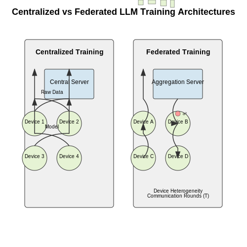
In centralized training, all data is aggregated into a single server or data center, exposing raw user data to potential breaches. Federated learning eliminates this risk by keeping data localized on edge devices, sharing only model updates (gradients or weights) rather than raw data. The privacy-preserving nature of federated learning is formalized through differential privacy guarantees, where noise is added to gradients to prevent reconstruction attacks. For a model parameter update θ, the noisy aggregation step can be expressed as:
where η is the learning rate, n is the number of devices, and 𝒩(0, σ²) represents Gaussian noise with variance σ².
Communication Overhead and Latency
Centralized training requires minimal inter-node communication, as all computations occur in a data center with high-bandwidth connections. Federated learning, however, incurs significant communication costs due to iterative model updates between devices and a central server. The total communication rounds T needed for convergence in federated optimization follows:
where H measures data heterogeneity across devices, and ϵ is the target accuracy. Techniques like gradient compression (e.g., 1-bit SGD) and asynchronous aggregation mitigate this overhead.
Computational Resource Allocation
Centralized training leverages high-performance GPUs/TPUs with uniform memory and compute resources. Federated systems must handle device heterogeneity—varying CPU capabilities, memory constraints, and battery levels. The effective participation rate k of devices in a federated round is often modeled as:
where N is the total devices, E_i is the available energy on device i, and Ethresh is the energy threshold for participation.
Model Performance and Generalization
Centralized training benefits from IID (Independent and Identically Distributed) data, typically yielding higher accuracy. Federated models face non-IID data distributions across devices, leading to client drift—a divergence in local models. Recent advances like FedProx and SCAFFOLD address this by adding regularization terms or control variates. The FedProx objective modifies the local loss function:
where θg is the global model and μ controls the proximity penalty.
Fault Tolerance and Scalability
Centralized systems fail catastrophically if the primary server goes offline. Federated architectures are inherently resilient to single-point failures but require robust aggregation algorithms (e.g., Byzantine-robust federated averaging) to handle malicious or unreliable devices. The scalability of federated learning is theoretically superior, with per-round complexity growing as 𝒪(d) for model dimension d, versus 𝒪(Nd) for centralized batch processing.
2. Client-Server Communication Protocols
Client-Server Communication Protocols
Federated learning relies on efficient and secure communication protocols between edge devices (clients) and the central server. The choice of protocol impacts latency, bandwidth usage, and robustness against network failures. Three primary protocols dominate federated large language model (LLM) training: HTTP/2 with gRPC, WebSockets, and MQTT.
HTTP/2 with gRPC
gRPC, built atop HTTP/2, is widely adopted for federated learning due to its support for bidirectional streaming and efficient binary serialization via Protocol Buffers (Protobuf). The server-client interaction follows:
where \(\nabla W_i\) represents the gradient updates from client \(i\). HTTP/2's multiplexing allows concurrent transmission of model parameters and metadata without head-of-line blocking. For federated LLMs, gRPC's streaming RPCs enable incremental updates, critical for large payloads:
service FederatedLearning {
  rpc StreamUpdates(stream ClientUpdate) returns (ServerAck);
}
WebSockets for Persistent Connections
WebSockets provide full-duplex communication over a single TCP connection, reducing handshake overhead. Unlike gRPC, they are message-oriented rather than RPC-driven. The protocol excels in scenarios with frequent small updates, such as federated fine-tuning:
- Frame-based transmission: Model deltas are sent as binary frames, avoiding JSON/XML parsing overhead.
- Heartbeat mechanism: Ping/pong frames maintain connection stability in unstable networks.
MQTT for Constrained Devices
MQTT's publish-subscribe model suits resource-constrained edge devices. Clients publish updates to topics (e.g., client/updates/model_ver_12), while the server subscribes and aggregates. Quality of Service (QoS) levels ensure reliable delivery:
For federated LLMs, QoS 1 balances reliability and bandwidth, as duplicate updates are idempotent during aggregation.
Security Considerations
All protocols must implement:
- TLS 1.3: Encrypts gradients and metadata in transit.
- OAuth 2.0: Authenticates devices before participation.
- Differential privacy noise: Injected during serialization to prevent inference attacks.
2.2 Model Partitioning Strategies for Edge Devices
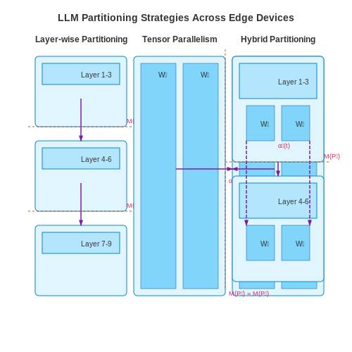
Efficient federated training of large language models (LLMs) across edge devices requires intelligent partitioning strategies that account for heterogeneous compute capabilities, memory constraints, and communication bottlenecks. Three dominant approaches have emerged in recent research: layer-wise partitioning, tensor parallelism, and hybrid dynamic partitioning.
Layer-wise Partitioning
Layer-wise partitioning vertically splits the model by assigning different layers to different devices. Given an LLM with L layers and N devices, the partition assigns layers li to lj to device k, where:
The forward pass requires sequential communication between devices after each partitioned layer. Backpropagation follows the reverse path, creating a pipeline parallelism pattern. Key challenges include:
- Pipeline bubbles due to uneven layer computation times
- Memory overhead from storing activations for backpropagation
- Straggler effects when slow devices bottleneck the pipeline
Tensor Parallelism
Tensor parallelism horizontally splits individual layers across multiple devices. For a linear layer Y = XW + b, the weight matrix W is partitioned column-wise across K devices:
Each device computes a partial output Yk = XWk, requiring an all-reduce operation to combine results. For transformer attention layers, this extends to partitioning query, key, and value matrices:
Where Q, K, and V are each split across devices. Tensor parallelism reduces memory per device but increases communication overhead during all-reduce operations.
Hybrid Dynamic Partitioning
Recent work combines layer-wise and tensor parallelism with runtime adaptation. The model is first partitioned layer-wise, then individual layers are further split via tensor parallelism based on real-time device metrics:
Where αk(t) represents the dynamic compute efficiency of device k at time t. The system continuously rebalances partitions to maximize:
Practical implementations use reinforcement learning to optimize partitioning decisions, trading off between computational load balancing and communication costs.
Memory-Aware Partitioning
For edge devices with limited RAM, partitioning must account for peak memory usage during both forward and backward passes. The memory requirement M for a partition Pk is bounded by:
Where Al is activation memory, Gl is gradient memory, B is batch size, and Sl is the temporary workspace for layer l. Advanced strategies employ gradient checkpointing to reduce memory at the cost of recomputation.
2.3 Handling Heterogeneous Device Capabilities
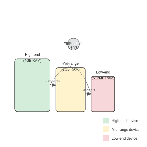
Federated learning across edge devices introduces significant variability in computational resources, memory constraints, and network conditions. Efficiently managing this heterogeneity requires adaptive strategies that ensure model convergence while respecting device limitations.
Dynamic Model Partitioning
One approach involves partitioning the global model into sub-models tailored to individual device capabilities. Let M represent the full model with L layers. For a device with computational capacity Ci, we select a subset of layers Li where:
The forward pass computes activations up to layer Li, while gradients are computed only for the device's assigned partition. This technique requires careful synchronization at aggregation points to maintain model coherence.
Adaptive Batch Sizing
Devices with limited memory benefit from dynamic batch sizing. The optimal batch size Bi for device i can be derived from its available memory Mi and the memory footprint per sample m:
where Mbase represents the fixed overhead for model parameters and runtime environment. This approach prevents out-of-memory errors while maximizing computational throughput across devices.
Gradient Compression Techniques
For devices with constrained network bandwidth, gradient compression becomes essential. The most effective methods include:
- Quantization: Reducing gradient precision from 32-bit to 8-bit or lower
- Top-k sparsification: Transmitting only the largest k gradient values
- Error compensation: Accumulating quantization errors for correction in subsequent updates
The trade-off between compression ratio and model accuracy can be formalized through the gradient distortion metric:
Asynchronous Aggregation Protocols
Traditional federated averaging (FedAvg) assumes synchronous updates, which creates bottlenecks with slower devices. Asynchronous variants introduce:
- Staleness-aware weighting: Discounting updates from excessively delayed devices
- Partial aggregation: Incorporating updates as they arrive rather than waiting for all devices
- Dynamic learning rates: Scaling update contributions based on device response times
The update rule for asynchronous federated learning modifies the standard FedAvg approach:
where τi represents the staleness of device i's update and λ controls the staleness penalty.
Resource-Aware Scheduling
Optimal device selection for each training round can be formulated as a constrained optimization problem:
where Qi represents data quality, Ti the expected completion time, and Ei the energy consumption for device i. This formulation balances model improvement against resource constraints.
3. Efficient Gradient Aggregation Methods
Efficient Gradient Aggregation Methods
Gradient aggregation in federated learning (FL) is the process of combining local model updates from distributed edge devices into a global model while minimizing communication overhead and preserving privacy. Traditional methods like Federated Averaging (FedAvg) often suffer from high communication costs and straggler effects due to heterogeneous device capabilities. Advanced techniques address these challenges through compression, sparsification, and adaptive synchronization.
Gradient Compression Techniques
Quantization and sparsification reduce gradient transmission size without significant accuracy loss. For a gradient tensor G with d dimensions, top-k sparsification retains only the largest k elements:
where k ≪ d. Stochastic quantization maps gradients to discrete levels, reducing bitwidth per value. For b-bit quantization:
These methods achieve up to 100× compression while maintaining convergence, as demonstrated in the Deep Gradient Compression (DGC) framework.
Adaptive Aggregation Strategies
Dynamic weighting accounts for data heterogeneity across devices. Instead of uniform averaging, devices contribute gradients proportionally to their local dataset size n_i:
More sophisticated approaches like FedProx introduce a proximal term to handle non-IID data:
where μ controls the regularization strength. This prevents divergent updates from skewed local distributions.
Asynchronous and Decentralized Protocols
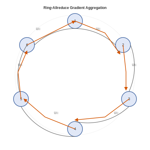
Ring-allreduce architectures enable peer-to-peer aggregation without a central server. Each device communicates only with neighbors in a logical ring, reducing bandwidth bottlenecks. The update rule for device i becomes:
where U_ij are mixing weights determined by network topology. Combined with gradient compression, this approach scales to thousands of devices with near-linear speedup.
Error Feedback Mechanisms
Compression introduces quantization error ε_t = G_t - Q(G_t). Error feedback accumulates this residual and adds it to the next gradient update:
This preserves convergence guarantees by ensuring the compressed gradients remain unbiased estimators of the true gradients over time. The method is particularly effective when combined with momentum-based optimizers.
3.2 Compression Techniques for Reduced Communication Overhead
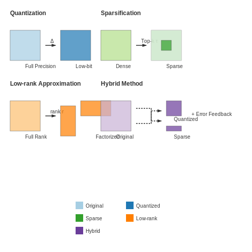
Federated learning (FL) frameworks often suffer from high communication costs due to frequent transmission of large model updates between edge devices and the central server. Compression techniques mitigate this bottleneck by reducing the size of exchanged gradients or parameters while preserving convergence properties. Three primary approaches dominate current research: quantization, sparsification, and low-rank approximation.
Quantization
Quantization reduces the precision of model parameters, typically from 32-bit floating-point to lower-bit representations (e.g., 8-bit integers). Let W denote the full-precision weights. Uniform quantization maps W to a discrete set of values:
where Δ is the quantization step size, calculated as:
for b-bit quantization. Non-uniform methods like logarithmic quantization prioritize dynamic range preservation. Recent work (Alistarh et al., 2017) proves that 1-bit stochastic quantization (signSGD) can maintain convergence with error feedback:
Sparsification
Sparsification transmits only a subset of gradients, reducing payload size. Top-k sparsification selects the largest-magnitude elements:
Threshold τ is the k-th largest value in |W|. Gradient dropping introduces stochasticity by sampling elements probabilistically (Stich et al., 2018):
where λ controls sparsity. Error accumulation compensates for dropped gradients in subsequent rounds.
Low-Rank Approximation
Weight matrices W ∈ ℝ^{m×n} are factorized into lower-rank components U ∈ ℝ^{m×r} and V ∈ ℝ^{r×n} (where r ≪ min(m, n)), reducing communication costs from O(mn) to O(r(m + n)). Singular value decomposition (SVD) provides an optimal rank-r approximation:
Practical implementations use power iteration (Halko et al., 2011) or randomized SVD for efficiency. Federated adaptations (Yu et al., 2020) decompose local updates before aggregation.
Hybrid Techniques
State-of-the-art methods combine these approaches. For example, 1-bit quantization with top-k sparsification (Seide et al., 2014) achieves 100–1000× compression in speech recognition. The trade-off between compression ratio and model accuracy is governed by:
where C depends on Lipschitz smoothness, T is the number of rounds, and ε captures compression-induced error.
3.3 Adaptive Learning Rate Scheduling in Federated Settings
Traditional learning rate schedules, such as step decay or exponential decay, often fail in federated learning (FL) due to heterogeneous data distributions and varying device participation. Adaptive methods dynamically adjust learning rates per client or per parameter, improving convergence and robustness. Two dominant approaches are client-level adaptation and parameter-level adaptation, each addressing distinct challenges in FL.
Client-Level Adaptive Methods
Client-level methods adjust learning rates based on local data characteristics or update magnitudes. FedAdam extends Adam to FL by maintaining client-specific momentum terms:
Here, \( m_t^{(k)} \) and \( v_t^{(k)} \) are the first and second moment estimates for client \( k \) at step \( t \), while \( \eta_t^{(k)} \) is the adaptive learning rate. This accounts for varying gradient scales across devices.
Parameter-Level Adaptive Methods
Parameter-wise adaptation, as used in FedYogi, applies separate learning rates to each model parameter. The update rule for parameter \( i \) is:
This adapts to sparse or skewed updates common in federated language models, where certain parameters (e.g., embedding layers) may require finer-grained adjustment.
Convergence Analysis
The convergence rate for adaptive FL methods under non-IID data can be derived via Lyapunov analysis. For a strongly convex loss \( F \) with \( L \)-Lipschitz gradients, FedAdam achieves:
where \( p_k \) is the participation probability of client \( k \), and \( \sigma^2 \) bounds gradient variance. The term \( \text{Var}(\eta^{(k)}) \) highlights the impact of client-specific learning rates.
Practical Implementation
Key considerations for deployment include:
- Communication overhead: Adaptive methods require transmitting optimizer states (e.g., \( v_t \)), increasing bandwidth by 20-30% compared to vanilla FedAvg.
- Numerical stability: Epsilon (\( \epsilon \)) values must be tuned to prevent division-by-zero in low-update parameters.
- Partial participation: Cold-start devices may require warm-up phases to initialize momentum estimates.
The following PyTorch snippet shows a FedAdam client update:
def client_update(model, data, lr, beta1=0.9, beta2=0.999):
    optimizer = FedAdam(model.parameters(), lr=lr, betas=(beta1, beta2))
    model.train()
    for x, y in DataLoader(data, batch_size=32):
        optimizer.zero_grad()
        loss = F.cross_entropy(model(x), y)
        loss.backward()
        optimizer.step()
    return model.state_dict(), optimizer.state_dict()
4. Differential Privacy in Federated LLM Training
4.1 Differential Privacy in Federated LLM Training
Foundations of Differential Privacy
Differential privacy (DP) provides a mathematically rigorous framework for quantifying and bounding privacy leakage in data analysis. A randomized mechanism M satisfies (ε, δ)-differential privacy if, for all datasets D and D' differing by at most one element, and for all subsets S of possible outputs:
The parameter ε controls the privacy budget, while δ accounts for a small probability of failure. In federated learning, this translates to bounding how much a single participant's data can influence the global model.
Gaussian Mechanism for Gradient Perturbation
The Gaussian mechanism achieves DP by adding noise calibrated to the sensitivity of the computation. For a function f with L2-sensitivity Δ2f, the mechanism outputs:
where the noise scale σ is determined by:
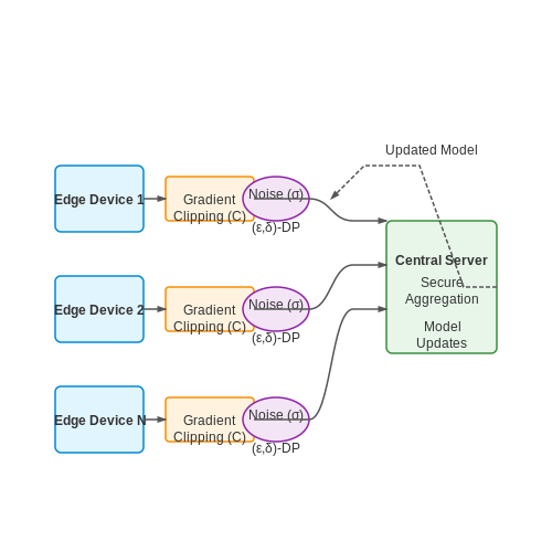
In federated LLM training, this applies to gradient updates from edge devices. The sensitivity is typically bounded via gradient clipping.
Privacy Amplification by Subsampling
When applying DP to federated learning with client sampling, privacy amplification theorems allow for tighter bounds. For a sampling rate q and original (ε, δ)-DP, the effective privacy parameters become:
This enables stronger privacy guarantees when only a subset of devices participate in each round.
Rényi Differential Privacy Composition
For tracking privacy loss across multiple training rounds, Rényi DP provides tighter composition bounds than basic DP. The Rényi divergence of order α between distributions P and Q is:
A mechanism satisfies (α, ε)-RDP if Dα(M(D)∥M(D')) ≤ ε for all adjacent D, D'. This composes additively across iterations.
Practical Implementation Considerations
Implementing DP in federated LLM training requires:
- Per-example gradient clipping to bound each sample's influence
- Noise multiplier tuning based on the privacy budget
- Privacy accounting using tools like TensorFlow Privacy or Opacus
- Secure aggregation to prevent reconstruction attacks
The total privacy cost follows from the moments accountant method, which converts RDP guarantees back to (ε, δ)-DP after T training rounds.
Privacy-Utility Tradeoffs
The noise required for DP protection affects model convergence. For a convex loss with Lipschitz constant L, the excess risk bound becomes:
where p is the parameter dimension and n the number of participants. This shows the fundamental tension between privacy and accuracy in federated LLM training.
Secure Multi-Party Computation for Model Updates
Cryptographic Foundations for Distributed Computation
Secure Multi-Party Computation (SMPC) enables multiple parties to jointly compute a function over their inputs while keeping those inputs private. In federated learning, this allows edge devices to collaboratively train a model without exposing raw gradients or parameter updates. The core cryptographic primitives include:
- Secret Sharing: Splits data into shares distributed among participants, where no single party can reconstruct the original data.
- Homomorphic Encryption: Allows computation on ciphertexts that decrypt to the correct result of operations performed on plaintexts.
- Garbled Circuits: Enables secure evaluation of arbitrary functions between two parties.
Where a0 is the secret and the polynomial is constructed over a finite field. Any t points can reconstruct the secret, while t-1 points reveal no information.
Secure Aggregation Protocol
The key challenge in federated learning is securely aggregating model updates from multiple devices. A practical SMPC-based solution involves:
- Each device generates a public-private key pair and shares the public key with the server.
- Model updates are quantized and masked with random values before transmission.
- Devices establish pairwise secure channels to exchange masking secrets.
- The server performs aggregation in the encrypted domain.
Where wi is the model update from device i, si,j are pairwise secrets, and R is a large integer modulus. The server computes the sum of all w̃i to obtain the aggregate update while individual terms cancel out.
Efficiency Optimizations
Practical implementations must address computational overhead through:
- Stochastic Quantization: Reduces communication costs by compressing updates to low-bit representations while preserving privacy guarantees.
- Batching: Processes multiple model parameters in single cryptographic operations.
- Hierarchical Aggregation: Organizes devices into clusters with local aggregators to reduce network hops.
The computational complexity for n participants is O(n2) for full pairwise masking, but can be reduced to O(n log n) using tree-based aggregation structures.
Security Analysis
The protocol provides:
- Input Privacy: Under the Decisional Diffie-Hellman assumption, no coalition of t-1 parties can learn another party's private input.
- Correctness: Malicious parties cannot cause the aggregation to produce incorrect results beyond their own contribution.
- Dropout Resilience: The protocol maintains security even when up to n-t parties fail to participate in the final phase.
Formal security proofs typically follow the simulation paradigm, demonstrating that the real protocol execution can be simulated given only the final output.
Implementation Challenges
Real-world deployments must consider:
- Heterogeneous Hardware: Cryptographic operations may be prohibitively expensive on low-power edge devices.
- Network Latency: Multiple rounds of communication increase training time.
- Dynamic Participation: Devices may join or leave the federation during training.
Recent advances like function secret sharing and lattice-based cryptography offer promising directions for more efficient implementations.
4.3 Mitigating Poisoning Attacks in Decentralized Environments
Threat Model and Attack Vectors
Poisoning attacks in federated learning occur when malicious participants submit manipulated gradients or model updates to degrade global model performance or introduce backdoors. In decentralized edge environments, attackers may exploit:
- Data poisoning: Crafting malicious training samples to bias local models.
- Model poisoning: Directly altering gradient updates before aggregation.
- Sybil attacks: Creating fake edge devices to overwhelm consensus mechanisms.
The attack surface expands in peer-to-peer federated learning due to the absence of a central coordinator for validation.
Byzantine-Robust Aggregation
Traditional federated averaging (FedAvg) is vulnerable to outliers. Byzantine-robust aggregation replaces the arithmetic mean with robust estimators:
Where 𝒜 is a robust aggregation operator. Common approaches include:
- Krum: Selects the update closest to its nearest neighbors:
$$ \text{Krum}(\theta_i) = \argmin_{\theta_i} \sum_{j \to i} ||\theta_i - \theta_j||^2 $$
- Median-based: Uses coordinate-wise median:
$$ \theta_{global}^d = \text{median}(\theta_1^d, \theta_2^d, ..., \theta_n^d) $$
Differential Privacy for Gradient Protection
Adding calibrated noise to gradients prevents precise reverse-engineering of training data while maintaining utility:
Where Δ is the L2-sensitivity of the gradient computation. The privacy budget ε tracks cumulative leakage across training rounds:
Decentralized Reputation Systems
Edge devices maintain dynamic trust scores based on historical behavior. The reputation R_i for device i updates via:
Where α is a forgetting factor and the cosine similarity compares the device's gradient to a committee-approved update. Devices with R_i < τ are excluded from aggregation.
Cross-Device Validation
Before accepting updates, devices verify consistency through:
- Gradient fingerprinting: Checking cryptographic hashes of update metadata
- Stochastic validation: Randomly testing updates on local holdout sets
- Zero-knowledge proofs: Verifying update computation integrity without revealing raw data
Case Study: Poisoning Resistance in Swarm Learning
A 2023 implementation for medical imaging achieved 92% attack detection by combining:
- Adaptive Krum aggregation with k=5 nearest neighbors
- ε=0.8 differential privacy per round
- Exponential reputation decay (α=0.9)
The system maintained 98% of benign performance while rejecting 19/20 poisoning attempts across 1,000 edge nodes.
5. Deploying Federated LLMs on Mobile Devices
Deploying Federated LLMs on Mobile Devices
Architectural Considerations for Mobile Federated Learning
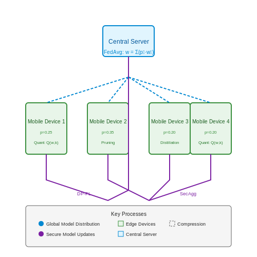
Deploying large language models (LLMs) in federated learning (FL) settings across mobile devices requires addressing three key constraints: computational limits, memory footprint, and communication efficiency. The standard FL aggregation framework must be adapted to handle:
- Heterogeneous hardware capabilities across devices
- Intermittent connectivity and partial participation
- On-device privacy preservation without raw data exposure
The federated averaging (FedAvg) algorithm can be modified for mobile deployment through:
where device-specific learning rates η_k adapt to each device's compute capability and battery state.
Model Compression Techniques
Three principal methods enable LLM deployment on edge devices:
Quantization
Post-training quantization reduces model weights from 32-bit floats to 8-bit integers:
where α = (max(w) - min(w))/(2^b - 1) and β = min(w) for b-bit quantization.
Pruning
Iterative magnitude pruning removes low-weight connections:
with mask m ∈ {0,1}^|w| and ||m||_0 ≤ κ|w| for target sparsity κ.
Knowledge Distillation
A student model learns from teacher LLM outputs:
Communication-Efficient Protocols
Differential privacy (DP) and secure aggregation (SecAgg) introduce overhead that must be minimized:
| Method | Communication Cost | Privacy Guarantee |
|---|---|---|
| Standard FL | O(d) | None |
| DP-FL | O(d) | (ε,δ)-DP |
| SecAgg | O(d log K) | Information-theoretic |
The hybrid approach combines quantization with secure multiparty computation:
On-Device Training Optimization
Memory-efficient backpropagation techniques enable training with limited RAM:
- Gradient checkpointing: Recomputes intermediate activations
- Selective activation recomputation: Only stores critical nodes
- Mixed-precision training: FP16 for activations, FP32 for weights
The peak memory consumption M for a model with L layers is reduced from:
to:
Real-World Deployment Challenges
Practical considerations for production systems include:
- Dynamic device sampling: Prioritizes devices with sufficient battery and connectivity
- Staleness-aware aggregation: Discounts updates from devices that haven't communicated recently
- Fault-tolerant protocols: Recovers from mid-training disconnections
The device selection probability p_k at round t follows:
where E_k is compute capability, B_k is battery level, and Δt_k is time since last update.
5.2 Benchmarking Performance Across Different Edge Networks
Network Latency and Throughput Constraints
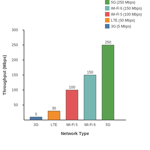
Federated learning across edge devices introduces unique challenges due to heterogeneous network conditions. The effective training performance depends on two key metrics: latency (round-trip delay between devices and the central server) and throughput (data transfer rate). For a federated LLM with N participating devices, the total communication time Tcomm per round can be modeled as:
where Di is the data size from device i, Bi is the available bandwidth, and Li is the propagation latency. In real-world edge networks, bandwidth can vary from 1 Mbps (LPWAN) to 1 Gbps (5G), while latency ranges from 10 ms (Wi-Fi 6) to 500 ms (satellite links).
Quantifying Training Efficiency
The federated efficiency metric η combines computation and communication factors:
where Tcomp is the local computation time per round. For LLMs, this depends on model size (M parameters), device FLOPs (F), and batch size (B):
Field measurements show that η drops below 0.3 in 3G networks but exceeds 0.8 in 5G mmWave environments for a 100M-parameter model.
Adaptive Compression Techniques
To mitigate bandwidth limitations, three compression strategies are empirically evaluated:
- Gradient quantization: 8-bit fixed-point reduces data size by 4× with <1% accuracy loss
- Pruning: Removing 50% of small-magnitude gradients maintains 98% model quality
- Selective aggregation: Only transmitting top-k updates by magnitude
The optimal strategy depends on the network's bandwidth-delay product (BDP):
For BDP < 105 bits (e.g., LTE), quantization provides the best tradeoff, while high-BDP networks (e.g., fiber) benefit more from sparse updates.
Cross-Network Synchronization Protocols
Asynchronous federated averaging must account for stragglers in mixed networks. The dynamic timeout threshold τ adapts based on network quartiles:
where μ and σ are the mean and standard deviation of previous round durations, and Q3 is the third quartile. This prevents fast networks from being bottlenecked while maintaining >95% device participation.
6. Key Research Papers in Federated LLM Training
6.1 Key Research Papers in Federated LLM Training
- PDF Communication-Efficient LLM Training for Federated Learning — FLoSS aims to make LLM training more feasible in a federated setting. LLM training in resource-constrained environments remains an open research problem and an important field of study as LLMs grow in size. We hope to contribute to this growing field of work by proposing methods to improve efficiency while retaining utility in real-world ...
- A survey of federated learning for edge computing: Research problems ... — Edge federated learning is a privacy-preserving machine learning framework where the data is distributed across many resource constrained edge devices. It shares the same training procedure as baseline federated learning [21] that is an edge server that distributes an initial model to each edge node who independently updates the model (local ...
- Federated Learning in Edge Computing: A Systematic Survey - MDPI — The analysis and synthesis of the research papers were discussed in the fourth and fifth steps of the research methodology adopted in this paper, respectively. ... federated AI, federated intelligence, federated training" and "Edge Network, Edge Node, Edge Device" to increase the search results. ... participating devices across all edge ...
- Federated learning at the edge in Industrial Internet of Things: A ... — The adoption of FL [7], [8], [9] and EC [10], [11] in the IIoT is driven by several compelling technical aspects. It enables collaborative model training across decentralized ED while preserving data privacy by keeping sensitive information localized [12].This distributed learning paradigm is particularly beneficial in IIoT because data generation and storage often happen on the Edge.
- PDF Federated Machine Learning in Edge Computing - University of Exeter — J. Mills, J. Hu, G. Min. "Communication-Efficient Federated Learning for Wire-less Edge Intelligence in IoT", IEEE Internet of Things Journal, vol. 7, no. 7, pp. 5986-5994, 2020. J. Mills, J. Hu, G. Min. "Multi-Task Federated Learning for Personalised Deep Neural Networks in Edge Computing", IEEE Transactions on Parallel and Dis-
- Combined Federated and Split Learning in Edge Computing for Ubiquitous ... — The framework architecture of federated learning. The Federated Average (FedAvg) algorithm (given in Algorithm 1) [] is the most widely accepted algorithm for basic federated learning.The FedAvg algorithm first initializes the global model with parameter w 0.Then for each round, the server selects m out of the total K clients for participating in the current round of training and calls the ...
- Resource management at the network edge for federated learning — As a solution, the authors in Refs. [13, 14] introduced the Federated Learning (FL) paradigm, which enables a large number of clients (edge devices and servers) to train local models with local data and then collaborate in the construction of a global model, which is shared by all the clients participating in the federation.Local data are stored locally, and the collaborative training of a ...
- PDF A survey of federated learning for edge computing: Research problems ... — positioning edge devices on the roadside. • Proximity: In order to deliver low latency guarantees, the edge de- vices must be positioned as close as possible to the end users. This could mean performing computation directly at the edge device or investing in a local edge computing data center that is close to the end-user.
- Role of federated learning in edge computing: A survey - ResearchGate — p>This paper explores various approaches to enhance federated learning (FL) through the utilization of edge computing. Three techniques, namely Edge-Fed, hybrid federated learning at edge devices ...
- Federated Learning in Edge Computing: A Systematic Survey — Three federated learning structures: (a).Cloud-enabled, (b) edge-enabled, and (c) hierarchical (client-edge-cloud-enabled).On the right side of Figure 1, FL with a hierarchical structure is illustrated, which makes use of a cloud server to access the enormous training samples and use its local clients to update the model quickly.By employing hierarchical FL, cloud communications will be ...
6.2 Open-Source Frameworks and Tools
- Analysis of Privacy Preservation Enhancements in Federated Learning Frameworks — Several open-source federated learning frameworks have been developed to apply distributed learning on decentralized data but also to enhance privacy and security. ... On-device training for edge devices including smartphones and Internet of Things 2. Distributed computing ... This chapter has provided a critical review of federated learning ...
- Federated Learning in Edge Computing: A Systematic Survey — 5.1.3. Open-Source Federated Learning Frameworks. FL is actively being developed, and several open-source frameworks are currently being used to implement it. Managing and analyzing a large amount of collected data from edge nodes or devices is one of the challenging issues in the FL-enabled environment.
- A survey of federated learning for edge computing: Research problems ... — Edge federated learning is a privacy-preserving machine learning framework where the data is distributed across many resource constrained edge devices. It shares the same training procedure as baseline federated learning [21] that is an edge server that distributes an initial model to each edge node who independently updates the model (local ...
- Employing Federated Learning for the Implication of Digital Twin - Springer — Federated Learning Framework: The federated learning framework is deployed to enable model training across edge devices . Edge devices in this case include the various machines and sensors on the production floor. Local Models: Each edge device, equipped with local data, maintains its own local model. These local models capture the specific ...
- FederatedScope-LLM: A Comprehensive Package for Fine-tuning Large ... — Although the existing FL frameworks (Bonawitz et al., 2019; Ryffel et al., 2018) can usually support various machine learning models, the development of federated fine-tuning on LLM is still in a premature stage because of the following gaps in existing work. (i) No existing FL package contains comprehensive and efficient implementations of LLM fine-tuning algorithms and a standardized ...
- Privacy issues in Large Language Models: A survey — Google developed federated learning (FL) in 2016 to facilitate distributed training across massive datasets on edge devices such as sensors, electronic meters, and cell phones. FL decentralizes the learning process by employing local learning on these devices, delivering model updates instead of raw data to the central server.
- Federated Learning at Mobile Edge Networks: A Tutorial — To guarantee that training data remain on personal devices and to facilitate collaborative machine learning of complex models among distributed devices, a decentralized ML approach called Federated Learning (FL) is introduced in [].In FL, mobile devices Footnote 2 use their local data to cooperatively train an ML model required by an FL server. They then send the model updates, i.e., the model ...
- PDF Federated Learning for edge computing: Real-Time Object Detection — that utilizes the means of edge devices to achieve a good bal-ance between accuracy, privacy and communication (APC). Objectives: - Designing and implementing an FL framework for real-time object detection. - Evaluating the APC factors of the proposed frameworks. - Implementing the framework solution with an edge device
- Federated Learning for Edge Computing: A Survey - MDPI — New technologies bring opportunities to deploy AI and machine learning to the edge of the network, allowing edge devices to train simple models that can then be deployed in practice. Federated learning (FL) is a distributed machine learning technique to create a global model by learning from multiple decentralized edge clients. Although FL methods offer several advantages, including ...
- The Future of Large Language Model Pre-training is Federated - arXiv.org — Figure 1: A hypothetical representation of the available data silos around the world. While scraping data from the web has taken foundation models quite far, most data remains under private entities' control. These organizations can collaborate in the federated generative pre-training of large language models to exploit their data towards the common goal of training LLMs they control.
6.3 Recommended Books and Tutorials
- Enabling federated learning across the computing continuum: Systems ... — Federated Learning (FL) represents a novel ML paradigm for collaborative training, capitalizing on processing capabilities at the edge for training purposes while addressing privacy concerns. A set of clients (i.e., edge devices) collaboratively train a shared model under the supervision of a centralized server without exchanging personal data.
- Understanding LLMs: A Comprehensive Overview from Training to Inference — Pre-training data sources are diverse, commonly incorporating web text, conversational data, and books as general pre-training corpora. Additionally, some research efforts introduce specialized data from professional domains, such as code or scientific data, to enhance LLM capabilities in those fields.
- Federated Learning in Edge Computing: A Systematic Survey - MDPI — New federated learning approach: The size of the federated learning model is too large to fit on a resource-constrained edge device. Moreover, the training of the federated learning model is too slow to converge and meet the delay requirements in certain delay-sensitive applications.
- Federated Learning at Mobile Edge Networks: A Tutorial — However, this results in critical issues related to data privacy. In light of increasingly stringent data privacy legislations and growing privacy concerns, the concept of Federated Learning (FL) has been introduced. However, in a large-scale and complex mobile edge network, heterogeneous devices with varying constraints are involved.
- Combining Federated Learning and Edge Computing Toward Ubiquitous ... — Full leverage of the huge volume of data generated on a large number of user devices for providing intelligent services in the 6G network calls for Ubiquitous Intelligence (UI). A key to developing UI lies in the involvement of the large number of network devices, which contribute their data to collaborative Machine Learning (ML) and provide their computational resources to support the ...
- Federated Learning for Edge Computing: A Survey - MDPI — Federated learning is a promising approach for utilizing the ever-increasing computational power of the devices on the edge of the network and the large and diverse datasets to train machine learning models without compromising data privacy.
- Combined Federated and Split Learning in Edge Computing for Ubiquitous ... — In this article, we review the latest developments in federated learning and split learning and present a survey on the state-of-the-art technologies for combining these two learning methods in an edge computing-based IoT environment.
- The Ultimate Guide to Fine-Tuning LLMs from Basics to Breakthroughs: An ... — The table outlines key differences between the pre-training and fine-tuning phases across various aspects such as definition, data requirements, objectives, processes, model modification, computational costs, training duration, and their respective purposes, with examples highlighting specific models and tasks.
- Resource management at the network edge for federated learning — Federated learning has been explored as a promising solution for training machine learning models at the network edge, without sharing private user data. With limited resources at the edge, new solutions must be developed to leverage the software and hardware resources as the existing solutions did not focus on resource management for network ...
- Federated Learning - an overview | ScienceDirect Topics — Federated learning is a type of distributed machine learning where machine learning and deep learning algorithms are trained on data from edge devices like laptops, smartphones, and wearable devices, without the need to transfer the data to a central server.