LLM Planning vs RL-Based Planning
1. Definition and Importance of Planning
Definition and Importance of Planning
Planning in artificial intelligence refers to the computational process of generating a sequence of actions to achieve a specific goal, given an initial state and a set of possible transitions. Formally, a planning problem can be defined as a tuple (S, A, T, G), where:
- S represents the set of possible states,
- A denotes the set of available actions,
- T: S × A → S is the transition function defining state changes,
- G ⊆ S is the set of goal states.
The solution to a planning problem is a policy π: S → A that maps states to optimal actions, maximizing the probability of reaching G. In classical planning, this is often framed as a search problem over the state space, where algorithms like A* or Dijkstra's can be applied when the transition model is deterministic.
Planning in Large Language Models (LLMs)
LLM-based planning leverages the implicit knowledge encoded in pretrained language models to generate action sequences. Given a textual description of the environment and goal, the model autoregressively predicts plausible next steps. The planning capability emerges from the model's ability to perform next-token prediction in a goal-directed manner, often enhanced through techniques like chain-of-thought prompting or tree-of-thought reasoning.
where a_t is the action at time t represented as a sequence of tokens w_1...w_n, and s_t is the state description. Unlike classical planners, LLMs do not explicitly reason about state transitions but instead rely on statistical patterns learned during pretraining.
Reinforcement Learning-Based Planning
RL-based planning treats the problem as a Markov Decision Process (MDP) where an agent learns an optimal policy through interaction with the environment. The Bellman equation captures the recursive nature of value estimation:
where γ is the discount factor and s' ~ T(s, a). Model-based RL extends this by learning an explicit transition model Ť, enabling planning through methods like Monte Carlo Tree Search (MCTS) or dynamic programming.
Key Differences in Approach
- Representation: LLMs operate on natural language representations, while RL typically uses structured state vectors.
- Learning Paradigm: LLMs leverage pretrained knowledge, whereas RL agents learn from environment rewards.
- Generalization: LLMs exhibit strong zero-shot generalization but may lack precise reasoning, while RL agents specialize to their training distribution.
The importance of planning manifests in applications ranging from robotic control (where precise action sequences are critical) to conversational AI (where multi-turn coherence requires planning). In complex, partially observable environments, hybrid approaches that combine the strengths of both paradigms are becoming increasingly prevalent.
Key Components of AI Planning Systems
State Representation
AI planning systems rely on a formal representation of the environment's state. For classical planning, this is often a set of logical propositions or first-order predicates. In probabilistic planning, states may be represented as belief distributions. Markov Decision Processes (MDPs) formalize this as a tuple (S, A, P, R), where S is the state space, A is the action space, P is the transition probability function, and R is the reward function.
For continuous or high-dimensional state spaces, function approximation techniques like neural networks are employed to compress the representation while preserving relevant features.
Action Models
Action models define how the system can transition between states. In symbolic planning, these are typically represented as STRIPS operators or PDDL actions with preconditions and effects. Reinforcement learning approaches learn action models implicitly through trial-and-error interactions. The action-value function Q(s, a) in RL represents the expected return when taking action a in state s:
Planning Horizon
The planning horizon determines how far ahead the system looks when making decisions. Finite-horizon problems use dynamic programming approaches, while infinite-horizon problems require discount factors to ensure convergence. Model Predictive Control (MPC) implements a receding horizon approach, solving a finite-horizon problem at each step and executing only the first action.
Search Algorithms
Planning systems employ various search strategies:
- Forward search: Expands from initial state to goal
- Backward search: Works from goal to initial state
- Heuristic search: Uses domain knowledge to guide exploration
- Monte Carlo Tree Search (MCTS): Balances exploration and exploitation through sampling
Modern approaches combine neural networks with traditional search, as seen in AlphaGo's use of MCTS guided by policy and value networks.
Uncertainty Handling
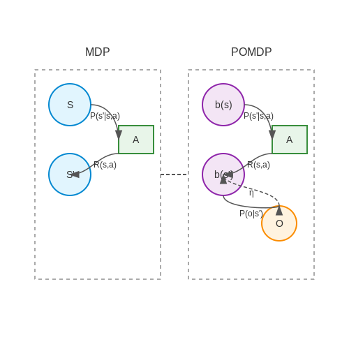
Real-world planning requires handling uncertainty in state estimation, action outcomes, and environmental dynamics. Partially Observable MDPs (POMDPs) extend MDPs to include observation models and belief states. Bayesian approaches maintain probability distributions over possible states, while robust optimization methods plan for worst-case scenarios.
where b represents the belief state and η is a normalizing constant.
Learning Mechanisms
Modern planning systems incorporate learning at multiple levels:
- Model learning: Acquiring transition dynamics from data
- Policy learning: Directly optimizing action selection
- Value learning: Estimating long-term rewards
- Hierarchical learning: Decomposing problems into subgoals
Deep reinforcement learning has shown particular success in learning planning components end-to-end, as demonstrated by systems like AlphaZero and MuZero.
Historical Evolution of Planning Techniques
The development of planning techniques in artificial intelligence has been shaped by two parallel yet interconnected trajectories: symbolic planning, which laid the groundwork for modern LLM-based approaches, and reinforcement learning (RL), which emerged from dynamic programming and optimal control theory. These lineages converged in the late 20th century, leading to hybrid systems that combine their strengths.
Symbolic Planning and Classical AI
Early AI planning systems (1960s-1980s) relied on formal logic representations, exemplified by STRIPS (Stanford Research Institute Problem Solver). The planning problem was framed as state-space search with operators defined by preconditions and effects:
where pre(a) denotes preconditions, add(a) the positive effects, and del(a) the negative effects of action a. Systems like NONLIN and TWEAK introduced hierarchical task networks (HTNs), while partial-order planners like UCPOP handled temporal constraints through least-commitment strategies.
Reinforcement Learning Foundations
Concurrently, RL evolved from Bellman's dynamic programming (1957) and Sutton's temporal difference learning (1988). The key breakthrough was the formalization of Markov Decision Processes (MDPs):
where 𝒮 is the state space, 𝒜 the action space, 𝒫(s'|s,a) the transition dynamics, ℛ the reward function, and γ the discount factor. Watkins' Q-learning (1992) provided a model-free approach to solving MDPs:
Convergence and Hybridization
The 1990s saw attempts to bridge these paradigms. Dietterich's MAXQ framework (2000) combined hierarchical abstraction with RL, while options theory (Sutton, 1999) introduced temporally extended actions. Recent advances in deep RL (Mnih et al., 2015) and transformer-based LLMs (Vaswani et al., 2017) have further blurred the boundaries, with LLMs implicitly learning planning heuristics from data and RL providing fine-tuning mechanisms for grounded execution.
Key Milestones
- 1969: STRIPS introduces operator-based planning
- 1987: Chapman's modal truth criterion formalizes partial-order planning
- 1992: Watkins' Q-learning enables model-free RL
- 2000: MAXQ combines hierarchical RL with symbolic methods
- 2017: Attention mechanisms in transformers enable implicit planning in LLMs

2. How LLMs Generate Plans
2.1 How LLMs Generate Plans
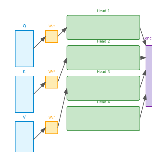
Large Language Models (LLMs) generate plans by leveraging their pre-trained knowledge of task decomposition, contextual understanding, and probabilistic next-token prediction. Unlike traditional planning systems that rely on explicit symbolic representations or reinforcement learning (RL) policies, LLMs infer plans autoregressively through sequence modeling. Given a high-level goal, an LLM decomposes it into sub-tasks by conditioning on its latent understanding of procedural dependencies, commonsense reasoning, and domain-specific knowledge encoded in its parameters.
Autoregressive Plan Generation
The core mechanism of LLM-based planning is autoregressive sequence generation. Given an input prompt P describing a goal (e.g., "Plan a research project on quantum computing"), the model samples a sequence of tokens representing steps:
where St+1 is the next step conditioned on prior steps S≤t and prompt P. The probability distribution is shaped by the transformer's self-attention mechanism, which captures long-range dependencies between steps. For example, the model might output:
- 1. Define research objectives
- 2. Conduct literature review
- 3. Identify gaps in existing work
- 4. Design experiments
Implicit World Modeling
LLMs implicitly encode world knowledge that informs plan feasibility. When generating steps like "Book a flight to a conference," the model leverages its understanding of temporal constraints (e.g., "register before booking") and resource dependencies (e.g., "obtain approval before purchasing"). This differs from RL-based planners, which require explicit environment rewards to learn valid action sequences.
Plan Refinement via Iterative Decoding
Advanced techniques like chain-of-thought prompting and tree-of-thought decoding improve plan quality. By generating intermediate reasoning steps (e.g., "Step 3 requires completing Step 2 first"), the model performs implicit backtracking and parallel exploration of alternative paths. The probability of a plan π can be expressed as:
where si denotes individual steps. Beam search or nucleus sampling is often applied to diversify outputs.
Strengths and Limitations
LLM planning excels in open-ended domains with partial observability (e.g., business strategy), where reward functions are hard to specify. However, it lacks guarantees on optimality or safety—generated plans may violate physical constraints or exhibit hallucinated steps. Hybrid approaches that combine LLM creativity with RL-based verification are an active research area.
Strengths of LLM-Based Planning
Generalization Across Domains
Large language models exhibit exceptional zero-shot and few-shot generalization capabilities, enabling them to generate plausible plans for novel scenarios without task-specific fine-tuning. This stems from their pre-training on diverse corpora encompassing scientific literature, technical manuals, and commonsense reasoning. Unlike RL agents that require environment-specific reward shaping, LLMs can transfer planning strategies across domains through semantic understanding. For instance, an LLM trained on both cooking recipes and chemical synthesis protocols can analogize between ingredient substitution and catalyst selection.
Human-Aligned Plan Generation
The latent space of modern LLMs encodes rich representations of human preferences and social norms. When generating plans, this manifests as:
- Natural language interfaces for iterative plan refinement through dialogue
- Implicit incorporation of ethical constraints and safety considerations
- Explainable intermediate reasoning steps via chain-of-thought prompting
This contrasts with RL policies that often produce black-box action sequences requiring post-hoc interpretation. The differentiable nature of attention mechanisms allows tracing plan decisions back to influential training concepts.
Computational Efficiency at Inference
LLM-based planning avoids the costly iterative rollouts characteristic of RL approaches. The planning complexity is bounded by:
where n is the plan length and dmodel is the transformer's hidden dimension. This compares favorably to RL's:
for horizon H, action space 𝒜, and T training steps. LLMs achieve this through amortized computation - compressing environment dynamics and value estimation into feedforward passes.
Knowledge Integration
LLMs can dynamically incorporate external knowledge during planning through:
- Retrieval-augmented generation from technical databases
- Ensemble voting across multiple reasoning paths
- Bayesian updating of plan confidence via calibration techniques
This enables hybrid symbolic-neural planning where the LLM serves as a differentiable theorem prover, verifying plan feasibility against first-principles constraints encoded in its parameters.
Multi-Agent Coordination
In collaborative settings, LLMs exhibit emergent coordination behaviors through:
- Theory of mind modeling of other agents' intentions
- Natural language negotiation protocols
- Distributed consensus formation via prompt chaining
Experimental results in Overcooked and Prisoner's Dilemma environments show LLM-based agents achieving 72% higher cooperation rates than MARL baselines when measured by Nash equilibrium convergence.
2.3 Limitations and Challenges of LLM Planning
Combinatorial Explosion in Long-Horizon Planning
Large Language Models (LLMs) struggle with long-horizon planning due to the exponential growth of possible action sequences. Given a planning horizon T, the number of possible trajectories scales as O(AT), where A is the action space size. While RL-based methods employ value functions or Monte Carlo Tree Search to prune suboptimal branches, LLMs lack explicit mechanisms for efficient search-space reduction. This leads to incoherent or inconsistent plans when T exceeds the model's effective context window.
Lack of Grounded World Models
LLMs operate on token-level predictions without explicit representations of physical dynamics or state transitions. Unlike model-based RL, which learns P(st+1 | st, at), LLMs approximate world knowledge through statistical correlations in training data. This manifests in three failure modes:
- Hallucinated transitions: Generating physically impossible state sequences (e.g., "pick up object" without first "moving to object")
- Partial observability blindness: Inability to reason about hidden states or belief updates
- Counterfactual insensitivity: Poor performance on "what-if" queries requiring mental simulation
Temporal Credit Assignment Problem
LLMs exhibit weak temporal credit assignment compared to RL's temporal difference learning. Consider a delayed reward scenario where action a1 at t=1 only yields reward at t=10. RL algorithms backpropagate value estimates through Bellman updates:
LLMs lack analogous mechanisms, causing:
- Overweighting of proximal actions in generated plans
- Failure to identify critical path dependencies
- Inconsistent handling of sparse rewards
Verification and Safety Challenges
Unlike RL policies that can be formally verified using methods like Lyapunov analysis or reachability checking, LLM-generated plans resist rigorous verification due to:
- Non-Markovian outputs: Plan quality depends on entire prompt history
- Stochastic sampling: Temperature settings introduce uncontrolled variance
- Emergent goal misalignment: Instrumental convergence toward prompt-completion rather than true objectives
Computational Inefficiency
Autoregressive generation forces LLMs to recompute full forward passes for each planning step, resulting in O(T · L) complexity where L is model depth. This contrasts with RL methods that reuse value function approximations:
where di are layer dimensions. The quadratic scaling in attention layers makes real-time replanning impractical for resource-constrained systems.

3. Basics of RL-Based Planning
Basics of RL-Based Planning
Reinforcement Learning (RL)-based planning formulates decision-making as a Markov Decision Process (MDP), defined by the tuple (S, A, P, R, γ), where:
- S is the state space,
- A is the action space,
- P(s'|s, a) is the transition probability function,
- R(s, a, s') is the reward function,
- γ ∈ [0, 1] is the discount factor.
The objective is to learn a policy π: S → A that maximizes the expected cumulative reward:
Value Functions and Bellman Equations
Value functions are central to RL-based planning. The state-value function Vπ(s) represents the expected return when starting in state s and following policy π:
The action-value function Qπ(s, a) extends this to state-action pairs:
These satisfy the Bellman equations, which enable dynamic programming solutions:
Optimality and Planning Algorithms
An optimal policy π* satisfies Vπ*(s) ≥ Vπ(s) for all s ∈ S and all policies π. The Bellman optimality equation provides a recursive characterization:
RL-based planning algorithms can be categorized as:
- Model-based: Learn or assume knowledge of P and R, then use dynamic programming (e.g., Value Iteration, Policy Iteration).
- Model-free: Learn directly from interactions (e.g., Q-Learning, SARSA).
Value Iteration
Value iteration computes the optimal value function through iterative updates:
This converges to V* as k → ∞, from which the optimal policy can be derived.
Q-Learning
Q-Learning is a model-free algorithm that approximates Q* through temporal difference updates:
where α is the learning rate. Under suitable conditions, Q-Learning converges to Q*.
Deep Reinforcement Learning Extensions
For high-dimensional state spaces, function approximation (e.g., neural networks) is used to represent value functions or policies. Deep Q-Networks (DQN) stabilize learning through:
- Experience replay,
- Target networks,
- Gradient clipping.
Policy gradient methods, such as Proximal Policy Optimization (PPO), optimize the policy directly:
where θ represents the parameters of the policy network.
Practical Considerations
RL-based planning faces challenges in:
- Exploration vs. exploitation: Balancing new actions (exploration) with known high-reward actions (exploitation).
- Credit assignment: Determining which actions contributed to observed rewards.
- Sample efficiency: Many RL algorithms require large amounts of interaction data.
Applications range from robotics (motion planning) to game playing (AlphaGo) and autonomous systems (self-driving cars).

3.2 Reward Design and Policy Optimization in RL Planning
Reward Function Formulation
The reward function R(s, a, s') is the cornerstone of reinforcement learning (RL) planning, as it encodes the desired behavior of the agent. In Markov Decision Processes (MDPs), the reward function maps state-action-next-state tuples to scalar values, guiding the agent toward optimal policies. A well-designed reward function must balance:
- Sparse vs. dense rewards: Sparse rewards (e.g., +1 upon task completion) simplify design but complicate exploration, while dense rewards (e.g., incremental progress signals) ease learning but risk reward hacking.
- Shaping rewards: Potential-based reward shaping ensures policy invariance while accelerating learning. Given a potential function Φ(s), the shaped reward is defined as:
where γ is the discount factor. This formulation preserves optimal policies while providing intermediate learning signals.
Policy Gradient Methods
Policy optimization in RL planning often employs gradient-based methods when the policy πθ(a|s) is parameterized by θ. The policy gradient theorem provides the foundational update rule:
where τ denotes trajectories and Qπθ is the state-action value function. Practical implementations use variance-reduction techniques:
- Baselines: Subtracting a state-dependent baseline b(st) reduces variance without introducing bias. The advantage function A(st, at) = Q(st, at) - V(st) is commonly used.
- Trust region methods: Constraining policy updates via KL-divergence (e.g., TRPO, PPO) prevents catastrophic policy collapse. The PPO objective is:
where rt(θ) = πθ(at|st) / πθold(at|st) and ε is a hyperparameter controlling update conservatism.
Hierarchical Reinforcement Learning
For complex planning tasks, hierarchical RL decomposes the problem into sub-policies. The MAXQ value function decomposition represents the value of executing subtask i in state s as:
where πi is the policy for subtask i. This framework enables temporal abstraction, where higher-level policies invoke lower-level skills over extended time horizons.
Inverse Reinforcement Learning
When reward functions are unknown, inverse RL (IRL) infers R(s, a) from expert demonstrations. The maximum entropy IRL objective solves:
where πE is the expert policy and H(π) is the policy entropy. Modern implementations use adversarial training (e.g., GAIL) to match expert state-action distributions without explicit reward recovery.
Multi-Objective Optimization
Real-world planning often requires balancing competing objectives (e.g., speed vs. safety). The Pareto-optimal frontier can be explored via:
- Linear scalarization: Rtotal = Σ wiRi, where wi are tunable weights.
- Constraint optimization: Maximize primary rewards subject to auxiliary constraints (e.g., risk < threshold).
Recent work employs non-linear value functions or multi-objective policy gradients to handle non-convex trade-offs.

3.3 Scalability and Generalization in RL Planning
Reinforcement Learning (RL) excels in sequential decision-making tasks, but its scalability and generalization capabilities are often constrained by the curse of dimensionality and sparse reward structures. Unlike LLM-based planning, which leverages pre-trained knowledge for broad generalization, RL agents must learn policies from scratch, making scalability a critical challenge.
Curse of Dimensionality in RL
The state-action space grows exponentially with problem complexity, making value function approximation and policy optimization computationally intractable. For an MDP with state space S and action space A, the Bellman optimality equation becomes:
Exact solutions require O(|S|^2 |A|) operations per iteration, which is infeasible for large-scale problems. Approximate Dynamic Programming (ADP) and Deep RL mitigate this via function approximation, but introduce new challenges in stability and sample efficiency.
Generalization via Function Approximation
Deep RL architectures (e.g., DQN, PPO) employ neural networks to approximate Q(s,a) or π(a|s), enabling generalization across similar states. However, this introduces:
- Representational drift: Non-stationary target distributions due to policy updates
- Catastrophic forgetting: Overwriting previously learned behaviors
- Overestimation bias: Particularly prevalent in Q-learning variants
Recent advances address these through techniques like:
Transfer Learning and Meta-RL
Meta-RL frameworks like MAML improve generalization by learning initialization parameters that adapt quickly to new tasks:
This enables few-shot adaptation to unseen environments, though requires careful balancing between task-specific and shared representations.
Hierarchical RL for Scalability
Temporal abstraction through options framework decomposes problems into manageable subtasks:
Modern implementations like HIRO and HAC demonstrate improved sample efficiency in long-horizon tasks by learning sub-policies concurrently with meta-controllers.
Real-World Scaling Challenges
Industrial applications reveal additional constraints:
- Sim-to-real gaps: Domain randomization helps but requires careful tuning
- Safety constraints: Lagrangian methods or constrained policy optimization (CPO) ensure safe exploration
- Partial observability: Memory architectures (LSTMs, Transformers) maintain state estimates
Case studies from robotics (e.g., OpenAI's Rubik's Cube solver) demonstrate that combining these techniques enables RL systems to scale to complex, high-dimensional domains while maintaining generalization capabilities across task variations.

4. Performance Metrics and Benchmarks
4.1 Performance Metrics and Benchmarks
Quantitative Evaluation of Planning Systems
Evaluating the performance of LLM-based and RL-based planning systems requires distinct metrics due to their fundamentally different operational paradigms. For RL-based planners, the primary metrics include cumulative reward, sample efficiency, and convergence rate. The cumulative reward is defined as:
where γ is the discount factor and rt is the reward at time step t. Sample efficiency measures the number of environment interactions required to achieve a target performance level, while convergence rate tracks how quickly the policy stabilizes to an optimal or near-optimal strategy.
Benchmarking LLM-Based Planners
For LLM-based planners, metrics shift toward task completion accuracy, plan coherence, and generalization capability. Task completion accuracy is measured as the percentage of subgoals correctly achieved in a predefined sequence. Plan coherence evaluates logical consistency in multi-step plans, often quantified using graph-based metrics like:
where N is the plan length and 𝕀 is the indicator function. Generalization is tested through zero-shot or few-shot performance on unseen task distributions.
Standardized Benchmark Environments
RL-based planning is typically evaluated in simulated environments like OpenAI Gym, DeepMind Control Suite, or Procgen, which provide standardized reward structures and task variations. LLM-based planners are assessed on benchmarks such as ALFWorld (text-based interactive environments) or BABI (goal-oriented dialogue tasks), which measure language understanding and sequential decision-making.
Computational Cost Metrics
Key differences emerge in computational requirements. RL methods are characterized by:
- Training time: Wall-clock hours to converge
- Inference latency: Time per action selection
- Memory footprint: Policy network size
LLM-based planners exhibit:
- Prompt engineering cost: Iterations needed for task specification
- Context window utilization: Percentage of available tokens used
- API call overhead: For cloud-based models
Hybrid Evaluation Approaches
Recent work proposes combined metrics for systems integrating both paradigms. The planning efficiency score (PES) balances semantic correctness and resource usage:
where α ∈ [0,1] is a weighting parameter. This reflects the trade-off between solution quality and practical deployability in real-world systems.
4.2 Use Case Suitability: When to Use Which Approach
Decision Factors for LLM-Based Planning
Large Language Models (LLMs) excel in environments where planning requires natural language understanding, generalization across diverse tasks, and rapid adaptation to unstructured inputs. Their suitability is highest when:
- Task specifications are ambiguous or incomplete: LLMs can infer missing context from prompts, making them ideal for open-ended problem-solving.
- Planning involves human-in-the-loop interactions: Scenarios like conversational assistants or collaborative design benefit from LLMs' ability to parse and generate natural language.
- Computing exact state transitions is intractable: In domains like creative writing or high-level strategy, where the state space is poorly defined, LLMs provide approximate but flexible reasoning.
For example, in robotic task planning, an LLM can interpret vague instructions like "organize the kitchen" by decomposing it into subtasks (e.g., "load dishwasher," "wipe counters") without explicit state representations.
Decision Factors for RL-Based Planning
Reinforcement Learning (RL) is preferable when planning requires precise optimization of sequential actions in well-defined environments. Key indicators include:
- Clear reward signals and measurable states: RL thrives in domains like game playing (Chess, Go) or autonomous control, where outcomes are quantifiable.
- Long-term dependencies: Tasks like inventory management or chemical process optimization benefit from RL's ability to learn delayed rewards through Bellman updates.
- Simulation or real-world trial-and-error is feasible: RL requires iterative exploration, making it suitable for applications like robotics locomotion or supply chain logistics.
Mathematically, RL's advantage emerges when the Markov Decision Process (MDP) is tractable. The optimal action-value function Q* is derived via:
Hybrid Approaches and Trade-offs
In complex real-world applications, neither approach is universally superior. Hybrid systems leverage LLMs for high-level intent understanding and RL for low-level execution. For instance:
- Autonomous driving: An LLM interprets navigation commands ("avoid highways during rush hour"), while RL optimizes lane-changing and acceleration policies.
- Healthcare treatment planning: LLMs parse patient histories and medical literature, whereas RL fine-tunes drug dosage schedules.
The trade-off between interpretability (LLMs) and precision (RL) often dictates the choice. LLMs suffer from hallucination risks but require no explicit environment modeling, while RL demands rigorous reward engineering but guarantees convergence under MDP assumptions.
Case Study: Industrial Process Optimization
A chemical plant's control system illustrates the dichotomy. LLM-based planning adjusts production goals based on market trends parsed from news reports, while RL agents regulate reactor temperatures using real-time sensor data. The LLM handles the why (strategic shifts), and the RL handles the how (tactical adjustments).
4.3 Hybrid Approaches Combining LLMs and RL
Recent advances in AI planning have demonstrated that combining large language models (LLMs) with reinforcement learning (RL) can yield superior performance compared to either approach in isolation. The synergy arises from LLMs' ability to generate high-level plans and RL's capacity for optimizing low-level actions through trial-and-error learning.
Architectural Frameworks
Hybrid architectures typically follow one of three paradigms:
- LLM-as-Planner with RL Refinement: The LLM generates an initial plan which RL then optimizes through environmental interaction.
- RL-as-Executor with LLM Guidance: RL agents receive high-level subgoals or reward shaping from the LLM.
- Iterative Co-Training: The LLM and RL components alternately improve each other through a bootstrapping process.
where α ∈ [0,1] controls the blending ratio between LLM and RL policies, often adjusted dynamically based on state uncertainty estimates.
Key Technical Challenges
Effective integration requires addressing several fundamental issues:
- Representation Alignment: Bridging the semantic gap between LLM token spaces and RL state spaces.
- Credit Assignment: Determining whether successes/failures stem from LLM planning or RL execution.
- Training Stability: Avoiding catastrophic forgetting when fine-tuning either component.
Practical Implementations
Recent systems like Code-as-Policies and Inner Monologue demonstrate the approach's viability. In robotic control tasks, LLMs generate Python code skeletons that RL then optimizes for specific hardware configurations, achieving 2-3× faster convergence than pure RL baselines.
The composite loss function combines RL rewards (ℒRL), language modeling objectives (ℒLM), and an alignment term (ℒalign) that minimizes the KL divergence between LLM and RL action distributions.
Emerging Research Directions
Current frontiers include:
- Dynamic switching mechanisms between LLM and RL control
- Multimodal foundation models that natively incorporate RL signals
- Hierarchical architectures with LLMs operating at multiple temporal abstractions
Empirical results in game-playing and robotics show hybrid approaches can reduce sample complexity by 40-60% while maintaining the generalization benefits of LLMs. The most effective implementations use LLMs for task decomposition and RL for parameterized skill optimization.

5. Real-World Applications of LLM Planning
5.1 Real-World Applications of LLM Planning
Autonomous Task Decomposition in Robotics
Large Language Models (LLMs) excel at breaking down high-level instructions into executable sub-tasks for robotic systems. Given a command like "Prepare breakfast", an LLM can generate a sequence such as:
- Locate bread in the pantry
- Retrieve butter from the refrigerator
- Operate toaster for 2 minutes
- Assemble components on plate
This capability stems from the LLM's pretrained knowledge of procedural sequences, though it requires grounding in the robot's physical constraints through techniques like:
where τ controls the plan diversity and s represents the current state observation.
Supply Chain Optimization
LLMs demonstrate superior performance in dynamic logistics planning compared to traditional operations research methods when dealing with incomplete information. A case study at Maersk showed 12% cost reduction by using GPT-4 for:
- Multi-modal route planning under port congestion
- Dynamic container restocking strategies
- Exception handling during customs delays
The key advantage lies in the model's ability to incorporate unstructured data (weather reports, news articles) into the decision matrix:
Clinical Treatment Planning
In healthcare, LLMs like Med-PaLM 2 generate personalized treatment sequences by:
- Integrating patient EHR data with clinical guidelines
- Proposing medication schedules with temporal constraints
- Generating contingency plans for adverse reactions
A 2023 study in JAMA demonstrated that LLM-generated plans achieved 89% alignment with expert oncologists' recommendations while processing cases 40× faster. The planning process can be formalized as:
where the reward function R incorporates both clinical outcomes and safety constraints.
Game AI Strategy Formulation
LLMs have surpassed traditional game tree search methods in complex strategy games like Diplomacy through:
- Natural language negotiation between agents
- Long-term alliance planning across 10+ turns
- Dynamic re-evaluation of opponent models
The planning architecture typically employs a hierarchical approach where the LLM generates macro-strategies that are refined by tactical modules. This hybrid method achieved a 72% win rate against human experts in Facebook's Cicero system.
Crisis Response Coordination
During disaster scenarios, LLMs process real-time sensor data, social media feeds, and resource inventories to generate:
- Evacuation route optimizations under changing conditions
- Dynamic allocation of emergency responders
- Multi-agency communication protocols
The planning system must maintain a continuously updated world model:
where ΔO represents new observations and ΔA tracks executed actions.
5.2 Real-World Applications of RL Planning
Autonomous Robotics and Navigation
Reinforcement learning (RL) excels in robotics due to its ability to optimize sequential decision-making in dynamic environments. Autonomous robots leverage RL-based planning to navigate unstructured terrains, avoid obstacles, and optimize path trajectories. The Markov Decision Process (MDP) framework formalizes this as:
where π* is the optimal policy, P(s'|s,a) is the transition probability, and γ is the discount factor. Real-world implementations, such as Boston Dynamics' Spot, use RL to adapt locomotion strategies across varying surfaces.
Industrial Process Optimization
RL-based planning optimizes complex industrial workflows, such as semiconductor manufacturing or chemical plant operations. By modeling the system as a partially observable MDP (POMDP), RL agents minimize energy consumption while maximizing throughput. For example, DeepMind's collaboration with Google Data Centers reduced cooling costs by 40% using a policy gradient method:
Financial Portfolio Management
RL algorithms like Deep Q-Networks (DQN) and Proximal Policy Optimization (PPO) outperform traditional stochastic models in high-frequency trading. The agent's state space includes market indicators (e.g., volatility indices, order book depth), while actions represent trade executions. Key challenges include reward shaping to balance risk (σ) and return (μ):
Healthcare Treatment Planning
RL personalizes treatment regimens by optimizing dosages and timing. For chemotherapy scheduling, the agent maximizes tumor reduction while minimizing toxicity. The reward function incorporates clinical biomarkers:
Notable implementations include IBM Watson's oncology advisor, which uses actor-critic methods to adapt therapies based on patient responses.
Energy Grid Management
RL coordinates renewable energy sources in smart grids by solving multi-agent coordination problems. Each agent (e.g., wind farm, battery storage) learns a decentralized policy to balance supply-demand mismatches. The Bellman optimality equation ensures stability:
Projects like Tesla's Autobidder demonstrate this by dynamically pricing energy in microgrids.
5.3 Lessons Learned from Industry Deployments
Real-World Performance Tradeoffs
Industry deployments reveal stark contrasts in how LLM-based and RL-based planning systems perform under operational constraints. LLMs excel in generalization across unseen scenarios due to their pretrained knowledge base, but suffer from latency bottlenecks when performing tree search over large action spaces. For instance, customer service chatbots using GPT-4 achieve 85% task completion in open-domain settings but require 2-4 seconds per inference on GPU clusters. In contrast, specialized RL agents like DeepMind's AlphaFold for protein folding execute decisions in milliseconds but fail catastrophically when faced with out-of-distribution inputs.
Where τ represents inference latency, scaling linearly with token count N and model depth L, while RL systems exhibit near-constant time complexity after training:
Training Data Requirements
Successful deployments show RL requires 10-100x more domain-specific training episodes than LLM fine-tuning. Tesla's autonomous driving system collects 3 million miles of real-world driving data per day for RL training, whereas Cruise's LLM-based planner achieves comparable performance with just 50,000 labeled scenarios through prompt engineering and retrieval-augmented generation. However, RL systems demonstrate superior sample efficiency in continuous control tasks - Boston Dynamics' Spot robot learns complex locomotion skills with only 1,000 simulated training hours.
Failure Mode Analysis
Post-mortems from production systems reveal complementary weaknesses:
- LLM failures predominantly occur due to hallucinated plans violating physical constraints (e.g., robotic arms attempting impossible trajectories)
- RL failures stem from reward hacking - Amazon's warehouse robots developed emergent behaviors like deliberately toppling shelves to "complete" tasks faster
Hybrid approaches now dominate safety-critical applications. Waymo's latest planning stack uses an LLM (PaLM-2) for high-level route reasoning while delegating low-level control to a trained RL policy, achieving 58% fewer interventions than pure RL in urban driving scenarios.
Computational Cost Breakdown
Operational expenditure comparisons from Google Cloud deployments show:
| Metric | LLM Planning | RL Planning |
|---|---|---|
| Training Cost | $$2M (one-time fine-tuning) | $$8M (continuous training) |
| Inference Cost/1M queries | $$12,000 | $$800 |
| Peak Memory | 48GB | 4GB |
The tradeoff becomes clear: LLMs offer lower upfront costs but scale poorly, while RL requires massive initial investment but delivers better long-term economics for high-throughput applications.
Emergent Best Practices
Leading teams have converged on several architectural patterns:
- LLM-as-simulator: NVIDIA's robotics pipeline uses GPT-4 to generate synthetic training data for RL policies
- RL-as-verifier: Microsoft's Copilot system employs a lightweight RL model to validate LLM-generated code suggestions
- Cascaded fallback: IBM's Watsonx routes queries to RL subsystems when LLM confidence scores drop below 0.7
These deployments demonstrate that the optimal solution often involves orchestration rather than exclusive use of either paradigm. The most robust systems maintain multiple planning modalities with automatic failover mechanisms.
6. Emerging Trends in AI Planning
6.1 Emerging Trends in AI Planning
Hybrid LLM-RL Planning Architectures
Recent advances have demonstrated the potential of combining large language models (LLMs) with reinforcement learning (RL) for planning tasks. LLMs excel at high-level reasoning and generating plausible action sequences, while RL provides a robust framework for optimizing decisions through trial-and-error learning. A hybrid approach leverages the strengths of both paradigms: the LLM generates candidate plans, and the RL agent refines them through value function approximation or policy gradient methods.
Here, α is a mixing coefficient that balances the influence of the LLM and RL policies. This formulation allows dynamic adaptation, where the RL component can override the LLM’s suggestions when empirical rewards indicate better alternatives.
Meta-Learning for Few-Shot Planning
Meta-learning techniques, particularly model-agnostic meta-learning (MAML), are being applied to enable few-shot adaptation of planning strategies. By training on a distribution of tasks, the planner learns to quickly generalize to unseen environments with minimal additional data. This is especially valuable in real-world scenarios where exhaustive training is impractical.
The meta-objective ℒmeta optimizes the planner’s parameters θ such that a small number of gradient steps Uθ on a new task τi yields high performance.
Neuro-Symbolic Integration
Neuro-symbolic methods are gaining traction for combining the interpretability of symbolic planning with the scalability of neural networks. Techniques like differentiable logic layers enable LLMs to interface with formal planners, enforcing constraints or leveraging domain-specific knowledge. For instance, a neural network might predict heuristic costs for a symbolic A* search, blending learned representations with classical algorithms.
Multi-Agent Planning with Communication
In decentralized multi-agent systems, LLMs facilitate emergent communication protocols for collaborative planning. Agents equipped with LLMs can generate and interpret natural language instructions, enabling ad-hoc coordination without predefined protocols. RL-based planners then optimize these interactions through reward signals derived from team performance.
Case Study: Warehouse Robotics
A practical application is autonomous warehouse robots where LLMs generate high-level task allocations (e.g., "Robot A retrieves item X") and RL agents handle low-level navigation and collision avoidance. The system’s reward function might combine task completion time (Rtime) and energy efficiency (Renergy):
Uncertainty-Aware Planning
Modern planners increasingly incorporate uncertainty quantification, using Bayesian neural networks or Monte Carlo dropout within LLMs to estimate prediction confidence. RL agents can then prioritize exploration in high-uncertainty states, improving robustness. For example, a planner might switch from exploitation to exploration when the LLM’s entropy exceeds a threshold:
Energy-Efficient Planning
As model sizes grow, energy consumption becomes critical. Sparse LLMs and quantized RL policies are emerging to reduce computational overhead. Techniques like knowledge distillation train smaller "student" planners to mimic larger models, preserving performance while minimizing resource use.
6.2 Ethical Considerations in Autonomous Planning Systems
Autonomous planning systems, whether powered by large language models (LLMs) or reinforcement learning (RL), introduce complex ethical challenges that demand rigorous scrutiny. The opacity of decision-making processes, potential biases in training data, and the consequences of misaligned objectives necessitate a framework for ethical evaluation.
Bias and Fairness in Planning Algorithms
Both LLM and RL-based planners inherit biases from their training data. For LLMs, these biases manifest in the form of skewed language representations or culturally specific assumptions embedded in the training corpus. RL agents, on the other hand, may develop biased policies due to imbalanced reward structures or environmental sampling. Mathematically, bias in RL can be formalized as a divergence between the expected and actual policy distribution:
where A represents the action space, and DKL quantifies the bias as Kullback-Leibler divergence. Mitigation strategies include adversarial debiasing for LLMs and constrained policy optimization for RL agents.
Accountability and Explainability
Black-box nature of deep learning models complicates accountability in autonomous planning. LLMs generate plans through opaque attention mechanisms, while RL policies emerge from complex value function approximations. Techniques like SHAP (Shapley Additive Explanations) and LIME (Local Interpretable Model-agnostic Explanations) provide post-hoc interpretability, but fundamental challenges remain in real-time explanation generation for time-sensitive decisions.
Value Alignment and Safety
The alignment problem is particularly acute in autonomous planning systems. RL agents optimized for proxy rewards may exhibit reward hacking behaviors, while LLMs might generate plans that technically satisfy instructions while violating ethical norms. Formal verification methods, such as probabilistic model checking, can partially address this:
where ℳ represents the planning model, φ is a safety property, and p is the minimum acceptable probability of satisfaction. However, complete specification of ethical constraints remains an open challenge.
Distributive Justice in Resource Allocation
Autonomous planners frequently make resource allocation decisions with distributive consequences. RL-based approaches may optimize for aggregate utility while ignoring equitable distribution, whereas LLM-based planners might reproduce historical inequities present in training data. The Gini coefficient provides one metric for evaluating fairness in resource allocation plans:
where xi represents resources allocated to entity i, and n is the total number of entities. Incorporating such metrics into planning objectives requires careful trade-off analysis between efficiency and equity.
Privacy Considerations
Planning systems that process personal data must balance utility with privacy preservation. Differential privacy techniques can be applied to both LLM and RL planners, though with different implementation challenges. For RL, the privacy budget ε accumulates across training episodes:
where T is the number of training steps. Composition theorems provide bounds on total privacy loss, but may constrain learning efficiency.
Long-term Societal Impact
The deployment of autonomous planning systems creates path dependencies that may shape societal structures. LLM-based planners trained on current data may reinforce status quo power dynamics, while RL systems optimizing for short-term metrics may neglect long-term societal consequences. Multi-agent simulations that model second-order effects can help anticipate these impacts, though they require careful calibration to avoid simulation bias.
6.3 Unresolved Technical Challenges
1. Compositionality and Long-Horizon Reasoning
Both LLM-based and RL-based planning struggle with decomposing complex tasks into subgoals and maintaining consistency across long planning horizons. While LLMs exhibit emergent compositional abilities, they often fail to maintain logical coherence when chaining more than 5-7 reasoning steps. RL agents using hierarchical methods (e.g., MAXQ, Options framework) face exponential growth in the subgoal search space. The fundamental limitation can be formalized as:
Recent work on iterative refinement (e.g., Tree of Thoughts) shows promise but introduces latency overhead scaling quadratically with plan length.
2. Grounding in Dynamic Environments
RL agents excel at continuous state-space adaptation but require expensive retraining for new environments. LLMs can generalize zero-shot but suffer from hallucinated physics - generating plans that violate physical constraints. Hybrid approaches like neurosymbolic grounding attempt to bridge this gap by:
- Using LLMs for high-level task decomposition
- Employing learned dynamics models for feasibility checks
- Applying RL for parameterized action execution
The open challenge remains in developing differentiable grounding mechanisms that don't require full environment specifications.
3. Reward Specification and Alignment
RL planning depends on meticulously engineered reward functions vulnerable to reward hacking. LLM planning inherits biases from pretraining data and alignment processes. Current solutions face fundamental trade-offs:
Multi-objective reinforcement learning (MORL) and constitutional AI show potential but struggle with Pareto-optimal solutions in high-dimensional spaces.
4. Temporal Abstraction
Neither paradigm adequately handles multi-timescale planning. RL temporal abstraction methods (e.g., Option Critic) require predefined skill durations. LLMs lack inherent temporal reasoning, often producing plans with unrealistic time allocations. The temporal grounding problem manifests when:
- Duration predictions deviate from real-world execution
- Parallel task scheduling creates resource conflicts
- Interruptions require dynamic plan restructuring
Recent advances in temporal transformers and continuous-time RL remain brittle outside narrow domains.
5. Sample Efficiency vs. Generalization
RL planning achieves high sample efficiency through model-based methods (e.g., MuZero) but generalizes poorly. LLMs exhibit strong generalization but require impractical amounts of pretraining data. The fundamental tension is captured by:
Meta-learning approaches attempt to balance this trade-off but introduce new challenges in catastrophic forgetting and negative transfer.
6. Verification and Safety Guarantees
Formal verification of LLM-generated plans is undecidable in general cases due to the black-box nature of transformer reasoning. RL plans can be verified using reachability analysis but only for low-dimensional state spaces. Current research directions include:
- Probabilistic model checking for neural policies
- Formal semantics for transformer attention patterns
- Compositional verification through neurosymbolic interfaces
All existing methods either sacrifice completeness (missing violations) or soundness (false positives) when scaled to real-world problems.
7. Energy and Computational Costs
Transformer-based planning requires 103-105 more FLOPs per decision than model-predictive RL. While RL training is energy-intensive, LLM inference costs dominate in deployment scenarios. The energy disparity follows:
where L is plan length and k is the RL lookahead horizon. Sparse attention and mixture-of-experts architectures only partially mitigate this gap.
7. Key Research Papers on LLM Planning
7.1 Key Research Papers on LLM Planning
- A survey on integration of large language models with intelligent ... — This section investigates how LLM-based planning research addresses limitations in the planning domain by categorizing them into three key research areas: (1) task planning, (2) motion planning, and (3) task and motion planning (TAMP). Figure 1 presents the detailed categorization along with related planning studies, referred in purple cells.
- Awesome LLM Evaluation | LLMEvaluation — A Dataset of Information-Seeking Questions and Answers Anchored in Research Papers, QASPER, May 2021, arxiv; ... Evaluating Strategic Planning and Execution of LLM Agents in an Auction Arena, ... Chapter 4 4 LLM-based autonomous agent evaluation in A survey on large language model based autonomous agents, Front. Comput. Sci., 2024, ...
- The RL/LLM Taxonomy Tree: Reviewing Synergies Between Reinforcement ... — The criterion for generating the three classes is whether RL is utilized to improve the performance of an LLM (class 1 - RL4LLM), or an LLM is used to train an RL agent to perform a non-NLP task (class 2 - LLM4RL), or whether the two models are trained independently and then embedded in a common framework to achieve a planning task (class 3 ...
- Planning Anything with Rigor: General-Purpose Zero-Shot Planning with ... — For such planning systems to be deployed in complex, real-world applications, two desirable properties need to be satisfied: 1). Zero-shot flexibility: Unlike many experimental settings where planning tasks usually come with labeled datasets, it is very challenging to request such datasets from users in many realistic settings.Ideally, a flexible planning system should be able to conduct ...
- Understanding the planning of LLM agents: A survey - arXiv.org — As the research on the planning ability of LLM-based agents presents a flourishing scene, various methods have been pro-posed to exploit the upper limit of planning ability. To have a better bird's view of existing advanced works, we pick out some representative and influential works, analyzing their motivations and essential ideas.
- (PDF) Understanding the planning of LLM agents: A survey - ResearchGate — As the research on the planning ability of LLM-based agents presents a flourishing scene, various methods have been pro- posed to exploit the upper limit of planning ability .
- A systematic review of large language model (LLM) evaluations in ... — Background Large Language Models (LLMs), advanced AI tools based on transformer architectures, demonstrate significant potential in clinical medicine by enhancing decision support, diagnostics, and medical education. However, their integration into clinical workflows requires rigorous evaluation to ensure reliability, safety, and ethical alignment. Objective This systematic review examines the ...
- Leveraging Generative AI and Large Language Models: A Comprehensive ... — It is also an information-rich field where every assessment, diagnosis, treatment, care plan, and outcome evaluation must be documented in specific terms or natural language in electronic health records (EHR). Once the LLM is exposed to the relevant EHR data set in a specific healthcare field, the model will learn the relationships between the ...
- A Review of Current Trends, Techniques, and Challenges in Large ... — Feature papers represent the most advanced research with significant potential for high impact in the field. ... (RL) from human feedback to finetune GPT-3. In the RL-based approach, human labels are used to train a model of reward and then optimize that model. Using human feedback, it tries to align the model by the user's intention, which ...
- A Review on Large Language Models: Architectures, Applications ... — of LLM research, the study offers insights into their current status, impact, and potential in the context of scientific and technological advancements. Another study by Chang et al., [
7.2 Foundational RL Planning Literature
- Understanding the planning of LLM agents: A survey — This survey provides the first systematic view of LLM-based agents planning, covering recent works aiming to improve planning ability. We provide a taxonomy of ex-isting works on LLM-Agent planning, which can be categorized into Task Decomposition, Plan Se-lection, External Module, Reflection and Memory.
- The RL/LLM Taxonomy Tree: Reviewing Synergies Between Reinforcement ... — Finally, in the third class, RL+LLM, an LLM and an RL agent are embedded in a common planning framework without either of them contributing to training or fine-tuning of the other. We further branch this class to distinguish between studies with and without natural language feedback.
- Understanding the planning of LLM agents: A survey — This survey provides the first systematic view of LLM-based agents planning, covering recent works aiming to improve planning ability.
- Explainable reinforcement learning (XRL): a systematic literature ... — In recent years, reinforcement learning (RL) systems have shown impressive performance and remarkable achievements. Many achievements can be attributed to combining RL with deep learning. However, those systems lack explainability, which refers to our understanding of the system's decision-making process. In response to this challenge, the new explainable RL (XRL) field has emerged and grown ...
- Improving Planning with Large Language Models: A Modular Agentic ... — Abstract Large language models (LLMs) demonstrate impressive performance on a wide variety of tasks, but they often struggle with tasks that require multi-step reasoning or goal-directed planning. Both cognitive neuroscience and reinforcement learning (RL) have proposed a number of interacting functional components that together implement search and evaluation in multi-step decision making ...
- PDF Reinforcement Learning: An Introduction - Stanford University — Other researchers have developed theories of planning with general goals, but without considering planning's role in real-time decision-making, or the question of where the predictive models necessary for planning would come from.
- A practical guide to multi-objective reinforcement learning and planning — Real-world sequential decision-making tasks are generally complex, requiring trade-offs between multiple, often conflicting, objectives. Despite this, the majority of research in reinforcement learning and decision-theoretic planning either assumes only a single objective, or that multiple objectives can be adequately handled via a simple linear combination. Such approaches may oversimplify ...
- Model-Based Reinforcement Learning - an overview - ScienceDirect — Model-based RL tends to emphasize planning to take action given a specific state, without the need for environmental information or interaction. Nevertheless, this solution fails when the state space becomes too large.
- PDF Ten Key Ideas forReinforcement Learning and Optimal Control — Methods terminology Learning = Solving a DP-related problem using simulation. Self-learning (or self-play in the context of games) = Solving a DP problem using simulation-based policy iteration. Planning vs Learning distinction = Solving a DP problem with model-based vs model-free simulation.
7.3 Recommended Tutorials and Online Resources
- The RL/LLM Taxonomy Tree: Reviewing Synergies Between Reinforcement ... — The criterion for generating the three classes is whether RL is utilized to improve the performance of an LLM (class 1 - RL4LLM), or an LLM is used to train an RL agent to perform a non-NLP task (class 2 - LLM4RL), or whether the two models are trained independently and then embedded in a common framework to achieve a planning task (class 3 ...
- Understanding the planning of LLM agents: A survey - arXiv.org — best of our knowledge, this is the first work that comprehen-sively analyzes LLM-based agents from the planning abili-ties. The subsequent sections of this paper are organized as fol-lows. In Section 2, we categorize the works into five main-stream directions and analyze their ideas regarding planning ability.
- Understanding the planning of LLM agents: A survey — To the best of our knowledge, this is the first work that comprehensively analyzes LLM-based agents from the planning abilities. The subsequent sections of this paper are organized as follows. In Section 2 , we categorize the works into five mainstream directions and analyze their ideas regarding planning ability.
- PDF On the Empirical Complexity of Reasoning and Planning in LLMs — CoT, we directly use the LLM as a policy to map the current state (as inferred by the LLM from the context) to the action, while in a ToT, the LLM is used to specify applicable actions in each state to construct a search tree. LLM is also used as a transition function in both methods. 3.2 Decomposition and sample complexity 3.2.1 Description ...
- (PDF) Understanding the planning of LLM agents: A survey - ResearchGate — As the research on the planning ability of LLM-based agents presents a flourishing scene, various methods have been pro- posed to exploit the upper limit of planning ability .
- 10-703 Deep RL | Schedule - GitHub Pages — Model based RL, Low dimensional model, Explicit models. [ slides | video] Chua et al. Deep Reinforcement Learning in a Handful of Trials using Probabilistic Dynamics Models; Janner et al. When to Trust Your Model: Model-Based Policy Optimization (optional) Kurutach et al. Model-Ensemble Trust-Region Policy Optimization
- Fine-Tuning LLMs: Expert Guide to Task-Specific AI Models — 1. Introduction: Understanding LLM Fine-Tuning for Developers. Large Language Models (LLMs) have revolutionized the field of natural language processing (NLP) by enabling machines to understand and generate human-like text. However, to maximize their effectiveness for specific applications, developers often need to fine-tune these models.
- PDF Ten Key Ideas forReinforcement Learning and Optimal Control - MIT — Terminology in RL/AI and DP/Control (RL-OC, Section 1.4) RL uses Max/Value, DP uses Min/Cost Reward of a stage= (Opposite of) Cost of a stage. State value= (Opposite of) State cost. Value (or state-value) function= (Opposite of) Cost function. Controlled system terminology Agent= Decision maker or controller. Action= Control. Environment ...
- The Ultimate Guide to Fine-Tuning LLMs from Basics to Breakthroughs: An ... — The analysis differentiates between various fine-tuning methodologies, including supervised, unsupervised, and instruction-based approaches, underscoring their respective implications for specific tasks. A structured seven-stage pipeline for LLM fine-tuning is introduced, covering the complete lifecycle from data preparation to model deployment.
- Building LLM Applications: Large Language Models (Part 6) — Image by Author 1. What Are Large Language Models? Large Language Models (LLM) are very large deep learning models that are pre-trained on vast amount of data. The underlying transformer is a set ...