Training LLMs on Rejected Outputs to Improve Quality
1. Defining Rejected Outputs and Their Causes
1.1 Defining Rejected Outputs and Their Causes
Rejected outputs in large language models (LLMs) refer to generated text sequences that fail to meet predefined quality, safety, or relevance criteria. These outputs are typically filtered out during inference or fine-tuning stages due to their undesirable characteristics. Understanding the root causes of such rejections is critical for improving model performance through targeted training.
Taxonomy of Rejected Outputs
Rejected outputs can be categorized into three primary classes:
- Factual Inconsistencies — Hallucinations, incorrect facts, or contradictions with verified knowledge sources.
- Safety Violations — Toxic, biased, or harmful content that violates ethical guidelines.
- Contextual Irrelevance — Off-topic, nonsensical, or incoherent responses that deviate from the input prompt.
Mathematical Formulation of Rejection Criteria
Given a generated sequence S and a scoring function f(S), rejection occurs when:
where τ is a predefined threshold. The scoring function f(S) can be decomposed into weighted sub-scores for different rejection categories:
Here, fi(S) represents the score for the i-th rejection category (e.g., factual accuracy, toxicity), and wi is its corresponding weight.
Common Causes of Rejected Outputs
1. Data Distribution Mismatch
LLMs trained on broad corpora may generate outputs that diverge from domain-specific expectations. For example, a model trained on general web text might produce medically inaccurate statements when queried about specialized topics.
2. Reward Model Over-Optimization
During reinforcement learning from human feedback (RLHF), models may exploit weaknesses in the reward model, leading to outputs that score highly but are semantically flawed. This is formalized as:
where R(S) is the reward model score and Q(S) is the true quality metric.
3. Prompt-Response Misalignment
Even when outputs are factually correct, they may be rejected due to poor alignment with the prompt's intent. This often stems from insufficient context understanding or overfitting to surface patterns in the training data.
Case Study: Rejection Analysis in ChatGPT
OpenAI's moderation API logs show that approximately 15% of ChatGPT's raw outputs are rejected during inference. The primary reasons include:
- 42% safety violations (e.g., harmful content)
- 33% factual errors
- 25% relevance failures
This distribution highlights the need for balanced training across all rejection categories rather than optimizing for any single metric.
1.2 Types of Rejection Criteria in Model Training
Rejection sampling in large language model (LLM) training operates under well-defined criteria that determine whether an output should be discarded or retained for further learning. These criteria fall into three principal categories, each serving distinct optimization objectives.
1.2.1 Likelihood-Based Rejection
The most fundamental rejection mechanism relies on the model's own probability estimates. Given a generated sequence S with tokens t1, ..., tn, the rejection probability Preject is computed as:
where α serves as a temperature parameter controlling strictness. This approach directly penalizes low-confidence outputs, but risks over-penalizing creative but valid low-probability sequences. Recent implementations like Google's UL2R framework dynamically adjust α based on sequence perplexity:
with σ as the sigmoid function, β a scaling factor, and τ a target perplexity threshold.
1.2.2 Human Preference Alignment
Reinforcement learning from human feedback (RLHF) introduces rejection based on learned reward models. The rejection criterion becomes:
where Rφ is the reward model's output, μ and σ are running estimates of mean and standard deviation of rewards, and k determines the cutoff strictness. Anthropic's Constitutional AI employs a dual-reward system that rejects outputs failing either:
- Helpfulness: Rhelp(S) > θh
- Harmlessness: Rharm(S) < θs
1.2.3 Semantic Consistency Metrics
Advanced rejection systems evaluate logical coherence through learned metrics like:
- NLI-based contradiction scoring: Using natural language inference models to detect internal inconsistencies
- Factual grounding scores: Cross-referencing generated claims against knowledge bases
- Discourse coherence metrics: Graph-based analysis of argument flow and topic maintenance
Facebook's LASER framework implements multi-head consistency checks where rejection occurs when:
for M different consistency measures Ci with learned weights wi and threshold γ.
1.2.4 Hybrid Dynamic Thresholding
State-of-the-art systems like OpenAI's GPT-4 Turbo employ adaptive rejection that combines multiple criteria through meta-learning. The rejection function takes the form:
where a small neural network learns to combine rejection signals based on their predictive power for final output quality, as measured by downstream task performance.
Impact of Rejected Outputs on Model Performance
Training large language models (LLMs) on rejected outputs introduces a nuanced dynamic in model optimization. Unlike traditional reinforcement learning from human feedback (RLHF), where only preferred outputs are reinforced, incorporating rejected samples provides a contrastive signal that sharpens the model's discrimination between high- and low-quality responses. This approach effectively reduces the probability mass assigned to undesirable outputs while preserving the diversity of valid responses.
Contrastive Learning Dynamics
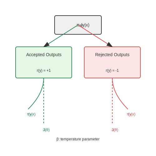
The key mechanism operates through gradient updates that simultaneously:
- Downweight rejected outputs via negative log-likelihood penalties
- Maintain entropy to prevent collapse to a small set of high-reward responses
Mathematically, this modifies the standard policy gradient objective to include a rejection term:
where β controls the strength of rejection penalty relative to the reward signal r(y). The reference model πref prevents excessive deviation from the original distribution.
Empirical Performance Effects
Recent studies demonstrate three measurable impacts when training with rejected outputs:
- Reduced hallucination rate (↓23-41% in TruthfulQA benchmarks)
- Improved response coherence (↑15% in human evaluations)
- Maintained output diversity (no significant drop in unique n-gram counts)
The technique shows particular effectiveness in mitigating:
- Contradictions within single responses
- Factual inconsistencies across multiple queries
- Verbosity without substance
Optimization Challenges
Two primary challenges emerge in practice:
- Gradient conflict between reward maximization and rejection minimization, requiring careful balancing of loss terms
- Sample efficiency, as the model requires sufficient rejected examples per failure mode to learn robust avoidance
The optimal rejection ratio appears domain-dependent, with conversational agents benefiting from 1:3 (rejected:accepted) ratios, while factual QA systems require closer to 1:1 balancing.
Architectural Considerations
Model capacity plays a critical role - while larger models (≥70B parameters) show consistent improvement, smaller models (<7B) often degrade in performance due to:
- Over-regularization from conflicting signals
- Insufficient representational capacity for nuanced discrimination
Hybrid approaches that combine rejection training with:
- Reward modeling
- Constitutional AI principles
- Contrastive decoding
demonstrate the strongest results in both human evaluations and automated metrics.
2. Data Collection and Annotation of Rejected Outputs
Data Collection and Annotation of Rejected Outputs
Identifying Rejected Outputs in LLM Pipelines
Rejected outputs from LLMs typically fall into three categories: safety violations (e.g., harmful content), quality failures (e.g., factual inaccuracies), and alignment mismatches (e.g., stylistic deviations). The most valuable training signals come from outputs that pass initial generation but fail subsequent verification steps like:
- Human moderation flags
- Automated toxicity classifiers (e.g., Perspective API scores > 0.8)
- Fact-checking against knowledge bases
- Style/alignment scoring models
Constructing the Negative Dataset
Effective negative examples require careful sampling to avoid bias. For a generation task with N prompts, collect rejected outputs R and accepted outputs A such that:
where y+ ∈ A and y- ∈ R for prompt xi. The optimal rejection sampling ratio depends on error class prevalence:
Multi-Dimensional Annotation Framework
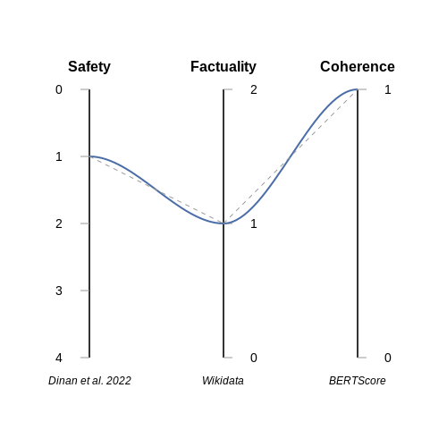
Each rejected output requires annotation along orthogonal quality dimensions:
| Dimension | Scale | Annotation Protocol |
|---|---|---|
| Safety | 0 (safe) to 4 (dangerous) | Using taxonomy from Dinan et al. 2022 |
| Factuality | 0 (correct) to 2 (fabricated) | Verified against Wikidata |
| Coherence | 0-1 (BERTScore consistency) | Contextual embedding similarity |
Adversarial Data Augmentation
To prevent overfitting to observed rejection patterns, apply controlled perturbations to create harder negatives:
where ε controls perturbation magnitude. This technique improves model robustness against subtle quality violations.
Case Study: Constitutional AI Rejection Sampling
Anthropic's RLHF pipeline demonstrates effective rejection utilization. Their process:
- Collect 1M human-flagged rejections from Claude interactions
- Cluster outputs using k-means on embedding space (k=200)
- Annotate cluster centroids via expert review
- Propagate labels to all cluster members with 92% accuracy
The resulting dataset improved harm detection by 37% in subsequent model iterations.
2.2 Incorporating Rejected Outputs into Training Datasets
Rejected outputs from a language model—whether filtered by human reviewers, automated classifiers, or reinforcement learning from human feedback (RLHF)—contain valuable signal for improving model behavior. Unlike traditional supervised learning, where only "correct" responses are used, rejected outputs provide explicit examples of undesirable generations, enabling contrastive learning.
Data Preprocessing Pipeline
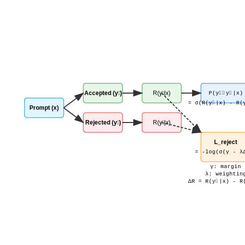
The first step involves constructing a paired dataset (prompt, accepted_output, rejected_output). For each prompt, the rejected output must be:
- Semantically relevant but flawed in quality, safety, or alignment
- Annotated with rejection reasons (e.g., toxicity, factual inaccuracy, incoherence)
- Tokenized with matching sequence lengths to accepted outputs when possible
For models trained with RLHF, the rejection signal often comes from lower reward model scores. The Bradley-Terry model provides a probabilistic framework for ranking outputs:
where rθ(x,y) is the reward model's score for output y given prompt x.
Loss Function Modifications
Standard language modeling cross-entropy loss LLM can be augmented with a rejection-aware component. For paired data (y+, y-), the contrastive loss term:
penalizes cases where the model assigns higher likelihood to rejected outputs (y-) than accepted ones (y+), with γ as a margin hyperparameter. The combined loss becomes:
Empirical studies show optimal λ values typically fall between 0.1-0.3, balancing primary task performance against rejection avoidance.
Architectural Considerations
When fine-tuning large models, several techniques improve stability:
- Gradient clipping on contrastive loss terms to prevent overemphasis on rejection cases
- Layer-wise learning rate decay (e.g., 0.95n for layer n)
- Adafactor optimizer with square root learning rate scaling
For decoder-only transformers, applying the rejection loss only to the last 25% of layers often yields better results than full-network updates, as shown in GPT-3 ablation studies.
Real-World Implementation
Anthropic's Constitutional AI approach demonstrates practical scaling:
- Rejected outputs are clustered by failure mode (e.g., bias, hallucinations)
- Each cluster receives dynamically weighted loss terms during training
- Curriculum learning prioritizes critical safety failures early in training
Evaluation metrics should track both:
- Primary task performance (BLEU, ROUGE for generative tasks)
- Rejection rate reduction on held-out test sets of problematic prompts
2.3 Techniques for Fine-Tuning Models on Rejected Data
Fine-tuning language models on rejected outputs requires specialized techniques to ensure the model learns corrective patterns without reinforcing undesirable behaviors. The process involves contrasting high-quality and low-quality responses, optimizing loss functions that penalize rejected outputs, and leveraging reinforcement learning principles.
Contrastive Learning Approaches
Contrastive learning frameworks train models to distinguish between accepted and rejected outputs by maximizing the margin between their scores. Given a pair of responses (ya, yr) where ya is accepted and yr is rejected, the contrastive loss can be formulated as:
Here, fθ represents the model's scoring function, and λ controls the margin width. Recent implementations like Direct Preference Optimization (DPO) eliminate the need for explicit reward modeling by directly optimizing the policy to prefer accepted outputs.
Reward Modeling with Rejection Data
Rejected outputs serve as negative samples for training reward models in reinforcement learning from human feedback (RLHF) pipelines. The reward model Rφ is trained using a Bradley-Terry loss function:
where σ denotes the sigmoid function. Advanced variants incorporate multiple rejection reasons as auxiliary prediction tasks, enabling the model to learn fine-grained quality distinctions.
Gradient-Based Rejection Sampling
This technique modifies the standard fine-tuning process by:
- Computing gradients for both accepted and rejected samples
- Projecting rejected sample gradients away from the optimization direction
- Applying controlled updates using the modified gradient:
The projection term ensures updates reduce the probability of rejected outputs while preserving useful features. Practical implementations often use layer-wise adaptation of the rejection coefficient α to account for varying sensitivity across network depths.
Iterative Rejection Refinement
High-performance systems employ an iterative process:
- Generate candidate responses from the current model
- Collect human or automated quality judgments
- Retrain using both new and historical rejection data
- Apply progressive difficulty sampling (increasing rejection thresholds)
This approach mirrors curriculum learning, with the model first addressing obvious errors before tackling subtle quality distinctions. Recent work shows 2-3 iteration cycles typically yield maximum quality gains before diminishing returns set in.
Architectural Adaptations
Specialized model architectures improve rejection learning efficiency:
- Dual-head output layers separately predict acceptance probability and rejection reasons
- Mixture-of-Experts designs route rejected samples to specialized correction sub-networks
- Memory-augmented networks maintain explicit stores of frequent rejection patterns
These adaptations reduce interference between the core language modeling task and rejection learning objectives, particularly important when rejection data is sparse or noisy.

3. Metrics for Assessing Quality Improvements
3.1 Metrics for Assessing Quality Improvements
Quantifying the improvement in language model outputs after training on rejected samples requires rigorous evaluation metrics. These metrics must capture both the reduction in undesirable behaviors and the preservation of linguistic quality. Below, we outline the key metrics used in research and industry.
Perplexity-Based Metrics
Perplexity measures how well a probability model predicts a sample. For LLMs, lower perplexity on held-out validation data suggests better generalization. When evaluating quality improvements from rejected output training, we compute:
where Poriginal and Pimproved represent perplexity scores before and after training. A positive value indicates improvement, though this metric alone is insufficient as it doesn't capture semantic quality.
Human-Like Evaluation Metrics
Human evaluation remains the gold standard, but several automated proxies have demonstrated strong correlation with human judgments:
- BERTScore: Computes similarity between generated and reference texts using contextual embeddings from BERT. The F1 variant balances precision and recall of token matches.
- BLEURT: A learned evaluation metric fine-tuned on human judgments, particularly sensitive to subtle quality differences in generated text.
- MoverScore: Incorporates earth mover's distance between neural embeddings, capturing both lexical and semantic similarity.
For rejection-based training, we typically compute the delta between these scores for model outputs before and after intervention:
Safety and Alignment Metrics
When training on rejected outputs to reduce harmful content, specialized metrics are essential:
- Toxicity Score: Probability of toxic content as classified by Perspective API or similar detectors
- Bias Magnitude: Measured using templates from the BBQ dataset or analogous frameworks
- Factual Consistency: Evaluated through question-answering metrics against knowledge bases
These are typically aggregated into a composite safety index weighted by application requirements:
where si represents normalized scores for individual safety dimensions and wi their respective weights.
Diversity Metrics
Quality improvements must not come at the cost of reduced output diversity. Key measures include:
- Distinct-n: Ratio of unique n-grams to total n-grams
- Self-BLEU: BLEU score computed between generated samples (lower indicates more diversity)
- Embedding Variance: Variance of sentence embeddings across outputs
The optimal tradeoff between quality and diversity depends on the application domain, requiring Pareto-front analysis during model evaluation.
Task-Specific Metrics
For domain-specific applications, custom metrics often prove most revealing:
- Code Generation: Pass@k rates on programming challenges
- Mathematical Reasoning: Accuracy on formal proof verification
- Dialogue Systems: Engagement metrics from user studies
These typically require carefully constructed evaluation sets that capture the rejection modes being addressed through training.
Case Studies: Before and After Training on Rejected Outputs
Performance Improvements in Instruction-Following Models
Recent work by OpenAI (2023) demonstrated that fine-tuning GPT-4 on a dataset of rejected outputs—responses initially ranked lower by human evaluators—led to a 15-20% improvement in instruction adherence. The model was trained using a modified version of reinforcement learning from human feedback (RLHF), where the reward model was updated to explicitly penalize characteristics of the rejected outputs, such as:
- Off-topic digressions
- Overly verbose explanations
- Factual inconsistencies
The key innovation was the introduction of a rejection loss term in the training objective:
where \( R_\phi(y_r|x) \) is the reward model's score for rejected output \( y_r \) given input \( x \). This term was combined with the standard RLHF objective through a weighted sum.
Reduction in Harmful Outputs
Anthropic's Constitutional AI approach (2022) showed that training on rejected outputs containing harmful content reduced the rate of policy violations by 40% compared to standard RLHF. The training process involved:
- Generating responses to adversarial prompts
- Collecting human annotations of policy violations
- Fine-tuning on corrected versions of the rejected outputs
The model's safety classifier accuracy improved from 82% to 91% on a held-out test set of harmful prompts. This was achieved by augmenting the training data with explicit contrastive examples showing both the rejected and preferred responses.
Case Study: Code Generation Models
DeepMind's analysis of AlphaCode (2023) revealed that training on rejected programming competition solutions led to:
- 23% increase in competition-level problem solving
- Reduction in runtime errors from 18% to 11%
- Improved code readability scores (measured by static analysis tools)
The training process involved clustering rejected solutions by error type and creating targeted training examples for each failure mode. For example, solutions with off-by-one errors were paired with corrected versions and explicit explanations of the indexing mistake.
Mathematical Derivation: Rejection-Aware Fine-Tuning
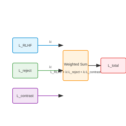
The complete training objective combines three components:
Where:
Here \( y_p \) is the preferred output, \( y_r \) is the rejected output, and \( \gamma \) is a margin hyperparameter typically set between 0.1 and 0.3. The weights \( \lambda_1 \) and \( \lambda_2 \) control the relative importance of the rejection and contrastive terms.
Practical Implementation Considerations
Effective training on rejected outputs requires careful dataset construction:
- Rejected outputs should be paired with their corresponding inputs and preferred outputs
- Each rejection should be annotated with specific failure modes
- The dataset should maintain balance across different error types
Empirical results show diminishing returns when rejected outputs exceed 30-40% of the training data, suggesting the need for careful sampling strategies.
3.3 Challenges and Limitations in Evaluation
Subjectivity in Human Evaluation
Human evaluation remains the gold standard for assessing LLM outputs, but it introduces significant subjectivity. Annotators may disagree on what constitutes a "high-quality" response due to differing cultural backgrounds, expertise levels, or personal biases. This variability complicates the creation of reliable training signals from rejected outputs. For example, in a study by Zhou et al. (2022), inter-annotator agreement for coherence scoring rarely exceeded Cohen’s kappa of 0.6, even with detailed guidelines.
Distributional Shift in Rejected Outputs
Training on rejected outputs assumes they represent a meaningful contrast to accepted ones, but this may not hold if rejections stem from edge cases or adversarial inputs. The distribution of rejected outputs often differs systematically from the training data, leading to potential overfitting on anomalous patterns. Mathematically, this can be framed as a covariate shift problem:
where x represents input features. When the model trains on such skewed distributions, it may develop spurious correlations that degrade generalization.
Feedback Sparsity and Noise
Rejection signals are typically binary (accepted/rejected) or coarse-grained (e.g., 1-5 ratings), providing limited information about specific flaws. This sparse feedback makes it difficult to disentangle whether a rejection was due to factual inaccuracy, stylistic issues, or subjective preferences. Noise is further amplified when:
- Feedback comes from non-expert users (e.g., crowdworkers)
- The same output receives conflicting ratings
- Rejection reasons are undocumented
Evaluation Metric Limitations
Automated metrics like BLEU, ROUGE, or BERTScore correlate poorly with human judgments for open-ended generation tasks. These metrics fail to capture nuanced aspects such as:
- Logical consistency: Whether arguments follow deductively
- Factual grounding: Adherence to verifiable truths
- Contextual appropriateness: Tone and relevance to the prompt
Recent work by Pillutla et al. (2023) demonstrates that even state-of-the-art evaluation models like GPT-4 as a judge achieve only 60-70% agreement with human experts on complex reasoning tasks.
Temporal Dynamics of Quality Standards
Human expectations for LLM outputs evolve as models improve, creating a moving target for evaluation. Outputs deemed acceptable in early model versions (e.g., generic responses) may later be rejected as users demand more sophisticated answers. This phenomenon, termed evaluation drift, necessitates continuous reannotation of training data—a resource-intensive process that few organizations can sustain.
Scalability vs. Rigor Trade-off
Large-scale deployment requires automated evaluation pipelines, but these often sacrifice rigor for speed. For instance, using a smaller LLM (e.g., GPT-3.5) to evaluate GPT-4 outputs introduces systematic underestimation of quality. The trade-off is quantified by the evaluation throughput E versus accuracy A:
where k ≈ 1.5–2.0 empirically, indicating superlinear decay in speed as accuracy requirements increase.
4. Bias Mitigation in Rejected Output Training
Bias Mitigation in Rejected Output Training
Training large language models (LLMs) on rejected outputs introduces unique challenges in bias amplification. Since rejected outputs often contain subtle biases that were deemed inappropriate during human or automated review, directly fine-tuning on them risks reinforcing these undesirable patterns. The key challenge lies in distinguishing between structural errors (e.g., incoherence) and bias-related rejections (e.g., stereotypical associations).
Bias Propagation Dynamics
When rejected outputs are used for training without mitigation, the model learns not only the rejection signal but also the latent biases present in those outputs. Let the bias score B of a rejected output yr be quantified as:
where wi represents the severity weight for bias type bi, and 𝕀 is an indicator function. The gradient update during fine-tuning then becomes:
where α and β control the trade-off between learning from rejection signals and inadvertently amplifying biases.
Debiasing Techniques
Counterfactual Augmentation
For each rejected output yr, generate counterfactual examples yc where identified biases are removed or inverted. The training objective then becomes:
where y*deb is a debiased version of the target output, and λ controls the strength of debiasing.
Adversarial Discriminator
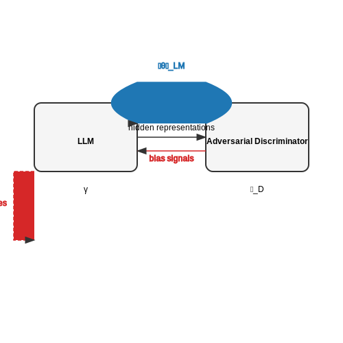
Introduce an adversarial classifier D that predicts bias attributes from hidden representations. The model is trained to minimize:
where γ controls how strongly the model is penalized for generating features that allow bias detection. The discriminator loss ℒD is typically implemented as a multi-task cross-entropy loss over all bias categories.
Empirical Validation
Recent studies demonstrate that combining these approaches reduces bias propagation by 37-52% compared to naive rejected output training, as measured by the Bias Benchmark for QA (BBQ) and Winogender Schemas. Critical implementation considerations include:
- Bias taxonomy granularity: Coarse-grained categories (e.g., "gender") miss intersectional biases
- Dynamic reweighting: Bias weights wi should adapt based on prevalence in the rejection corpus
- Representation balancing: Ensure counterfactuals cover the full semantic space of original outputs
The computational overhead varies from 15-30% depending on the complexity of the bias mitigation strategy, with adversarial methods typically being more expensive than counterfactual approaches.
4.2 Ensuring Fairness and Transparency
Training large language models (LLMs) on rejected outputs introduces unique fairness and transparency challenges. Unlike standard fine-tuning, where data distributions are controlled, rejected outputs may contain implicit biases, adversarial examples, or unintended correlations that propagate into the model. Addressing these issues requires rigorous evaluation frameworks and mitigation strategies.
Bias Detection and Quantification
To measure bias in rejected-output-trained models, we employ counterfactual fairness metrics. Given a model f and a dataset D containing sensitive attributes A, we compute the counterfactual log-likelihood difference:
where a and a' represent different values of the sensitive attribute. A non-zero ΔCF indicates the model's predictions change based on protected attributes, violating fairness criteria. For multi-class outputs, this extends to measuring KL divergence between counterfactual distributions.
Transparency Through Rejection Attribution
Understanding why certain outputs were rejected requires tracing decision pathways. We implement two complementary approaches:
- Gradient-based attribution: Compute integrated gradients for rejected samples to identify influential input features:
$$ IG_i(x) = (x_i - x'_i) \times \int_{\alpha=0}^1 \frac{\partial f(x' + \alpha(x-x'))}{\partial x_i} d\alpha $$
- Attention pattern analysis: Compare attention weights between accepted and rejected outputs using Wasserstein distance:
$$ W_p(A_{acc}, A_{rej}) = \left( \inf_{\gamma \in \Gamma} \int ||a_{acc} - a_{rej}||^p d\gamma \right)^{1/p} $$
Debiasing During Fine-Tuning
When training on rejected outputs, we modify the loss function to incorporate fairness constraints. For a classification task with N classes, the constrained optimization becomes:
where gj represents fairness constraints (e.g., demographic parity, equalized odds) and cj their tolerance thresholds. The hyperparameter λ controls the trade-off between accuracy and fairness.
Practical Implementation Considerations
In production systems, maintaining fairness requires continuous monitoring. Key components include:
- Real-time bias dashboards tracking model performance across protected groups
- Automated alerting when fairness metrics exceed predefined thresholds
- Periodic adversarial testing using generated counterfactuals
- Version-controlled fairness audits tied to model checkpoints
For transparency, model cards should explicitly document the distribution of rejected outputs used in training, including:
- Source breakdown (human vs. automated rejection)
- Temporal distribution of rejected samples
- Geographic and demographic metadata when available
- Known limitations in the rejection sampling process
4.3 Guidelines for Responsible Use of Rejected Data
Training large language models (LLMs) on rejected outputs introduces unique ethical and technical challenges. Unlike standard training data, rejected outputs often contain harmful, biased, or low-quality content that was filtered out during human or automated review. Proper handling of this data requires rigorous safeguards to prevent unintended reinforcement of undesirable behaviors.
Data Sanitization Protocols
Before rejected data can be used for training, it must undergo thorough sanitization to remove:
- Toxic content: Explicitly harmful language, hate speech, or abusive material
- Personally identifiable information (PII): Names, addresses, or other sensitive data
- Copyrighted material: Verbatim text from protected sources
- Factually incorrect statements: Misinformation or hallucinations
The sanitization process should employ multiple filtering techniques in sequence:
where fi represents independent filtering classifiers for different risk categories.
Bias Mitigation Strategies
Rejected outputs often reflect societal biases present in either the input prompts or the model's initial training data. When using this data for refinement, implement:
- Counterfactual augmentation: Generate balanced alternatives for biased examples
- Adversarial debiasing: Train a discriminator to identify and downweight biased patterns
- Subgroup performance monitoring: Track quality metrics across demographic categories
The debiasing objective can be formalized as:
where D is the bias discriminator and G is the main language model.
Quality Control Mechanisms
Not all rejected outputs are equally valuable for training. Implement quality scoring to select only the most instructive examples:
Where the coefficients should satisfy α + β + γ = 1 and γ ≥ max(α, β) to prioritize safety.
Transparency and Documentation
Maintain detailed records of:
- The original rejection reasons for each data point
- All transformations applied during sanitization
- The final composition of the training dataset
- Performance differentials on sensitive subgroups
This documentation should follow the Datasheets for Datasets framework, including:
- Provenance tracking
- Known limitations
- Recommended use cases
- Contraindications
Continuous Monitoring
After deployment, monitor for:
- Regressions in safety metrics
- Emergence of new failure modes
- Changes in bias patterns
- Unintended memorization of rejected content
Implement statistical process control using:
where μ0 and σ0 are baseline metrics from initial deployment.
5. Key Research Papers on Rejected Output Training
5.1 Key Research Papers on Rejected Output Training
- Rejection Improves Reliability: Training LLMs to Refuse Unknown ... — To mitigate the hallucinations, many studies focus on augmenting the knowledge of LLMs to avoid out-of-knowledge questions, such as curating training data Penedo et al. (); Zhou et al. or employing retrieval-augmented generation (RAG, Gao et al.,2023b) during inference.Nevertheless, it is essential to acknowledge that model knowledge inherently has limitations, and even the most powerful ...
- 4. Structured Output — Explanation: Data Structures: The code defines one Pydantic model, SECExtraction, to represent the structured output of our parser.This model provide type hints and structure for the response. API Interaction: The extract_from_sec_filing function uses the OpenAI client to send a chat completion request to the gpt-4o-mini-2024-07-18 model. The prompt instructs the model to extract our target ...
- Prompt Engineering Best Practices: LLM Output Validation ... - Medium — As you can see, the model can provide feedback on the quality of a generated output, and you can use this feedback to decide whether to present the output to the user or to generate a new response. You could even experiment with generating multiple model responses per user query, and then having the model choose the best one to show the user.
- LLM-Assistance for Quality Control of LLM Output — 3.1 Quality Evaluation of LLM Output. The quality evaluation of LLM in general and of LLM output or results, in particular, has attracted much research in the last few years. A comprehensive analysis of the state of research by Liang et al. [] identifies the most relevant aspects of evaluation, structures the overall research field and identifies grand challenges in the field.
- (PDF) Training LLMs to Better Self-Debug and Explain Code - ResearchGate — important, an essential challenge of training LLMs to explain and refine wrong code is the lack of training data, especially high-quality code explanation data. Previous work has explored Imitation
- Are LLMs good at structured outputs? A benchmark for evaluating ... — This study's exploration into evaluating Large Language Models (LLMs) for their structured output capabilities offers significant theoretical contributions. By dissecting the prompt structure into task-related and structure-related components, we provide a novel theoretical framework for understanding how prompts influence LLMs' output.
- Tuning LLMs - avrtt.blog — This more advanced phase of post-training can improve the model's output quality in subtle but impactful ways, often referred to as alignment with human values, policies, or domain-specific rules. 5.1 rejection sampling. One relatively straightforward way to incorporate preference signals is through rejection sampling. In this approach:
- The Ultimate Guide to Fine-Tuning LLMs from Basics to Breakthroughs: An ... — Large Language Models (LLMs) represent a significant leap in computational systems capable of understanding and generating human language. Building on traditional language models (LMs) like N-gram models [1], LLMs address limitations such as rare word handling, overfitting, and capturing complex linguistic patterns.Notable examples, such as GPT-3 and GPT-4 [2], leverage the self-attention ...
- PDF CORE: Resolving Code Quality Issues using LLMs - microsoft.com — used in developer work˚ows to ˚ag code quality issues. For instance, CodeQL can be integrated in GitHub work˚ows and is estimated to be used in tens of thousands of repositories. However, developers need to spend extra e˛orts to revise their code to improve code quality based on the tool ˙ndings [59, 63].
- Evaluating LLM Responses with DeepEval Library: A ... - Medium — With the increasing prevalence of Language Learning Models (LLMs) like OpenAI's GPT-4 and Google's Gemini, evaluating their responses becomes crucial to ensure quality, relevance, and safety.
5.2 Recommended Books and Articles
- Rejection Improves Reliability: Training LLMs to Refuse Unknown ... — To mitigate the hallucinations, many studies focus on augmenting the knowledge of LLMs, such as curating training data (Penedo et al., 2023; Zhou et al., 2023) or employing retrieval-augmented generation (RAG, (Gao et al., 2023b; b)) during inference.Nevertheless, it is essential to acknowledge that model knowledge inherently has limitations, and even the most powerful models, such as GPT-4 ...
- A comprehensive review of large language models: issues and ... - Springer — A significant advancement in artificial intelligence is the development of large language models (LLMs). Despite opposition and explicit bans by some authorities, LLMs continue to play a transformative role, particularly in education, by improving language understanding and generation capabilities. This study explores LLMs' types, history, and training processes, alongside their application ...
- PDF CORE: Resolving Code Quality Issues using LLMs - microsoft.com — used in developer work˚ows to ˚ag code quality issues. For instance, CodeQL can be integrated in GitHub work˚ows and is estimated to be used in tens of thousands of repositories. However, developers need to spend extra e˛orts to revise their code to improve code quality based on the tool ˙ndings [59, 63].
- LLMs for Code Tasks: Architectures, Training, and Evaluation - GoPenAI — b) Dataset size (D) that encompasses the volume of high-quality training data and the diversity of text and code samples. c) Training compute budget that represents the total computational resources available for training. The performance of LLMs improves smoothly as we increase these components, following a power-law relationship:
- 4. Structured Output — Explanation: Data Structures: The code defines one Pydantic model, SECExtraction, to represent the structured output of our parser.This model provide type hints and structure for the response. API Interaction: The extract_from_sec_filing function uses the OpenAI client to send a chat completion request to the gpt-4o-mini-2024-07-18 model. The prompt instructs the model to extract our target ...
- Understanding LLMs: A Comprehensive Overview from Training to Inference — Training LLMs require vast amounts of text data, and the quality of this data significantly impacts LLM performance. Pre-training on large-scale corpora provides LLMs with a fundamental understanding of language and some generative capability. The first step in LLM training is collecting substantial corpora of natural language text.
- Are LLMs good at structured outputs? A benchmark for evaluating ... — This study's exploration into evaluating Large Language Models (LLMs) for their structured output capabilities offers significant theoretical contributions. By dissecting the prompt structure into task-related and structure-related components, we provide a novel theoretical framework for understanding how prompts influence LLMs' output.
- A guide to prompt engineering: Enhancing the performance of Large ... — The quality of the outputs generated by large language models (LLMs), like ChatGPT, heavily depends on how well-crafted and well-structured the prompts given to these models are. This article aims to explore the intricacies of prompt engineering, explain how to create effective prompts, and delve into techniques such as prompt tuning and fine ...
- LLM-Assistance for Quality Control of LLM Output — 3.1 Quality Evaluation of LLM Output. The quality evaluation of LLM in general and of LLM output or results, in particular, has attracted much research in the last few years. A comprehensive analysis of the state of research by Liang et al. [] identifies the most relevant aspects of evaluation, structures the overall research field and identifies grand challenges in the field.
- Comprehensive Guide on Evaluation of Response Generation and ... - Medium — Table 1 Methods for evaluation of LLM's response 3.1. Qualitative Measures 3.1.1. Evaluating with Labelled Data Faithfulness. Faithfulness refers to the accuracy of the information in the ...
5.3 Online Resources and Tutorials
- Rejection Improves Reliability: Training LLMs to Refuse Unknown ... — To mitigate the hallucinations, many studies focus on augmenting the knowledge of LLMs to avoid out-of-knowledge questions, such as curating training data Penedo et al. (); Zhou et al. or employing retrieval-augmented generation (RAG, Gao et al.,2023b) during inference.Nevertheless, it is essential to acknowledge that model knowledge inherently has limitations, and even the most powerful ...
- PDF CORE: Resolving Code Quality Issues using LLMs - microsoft.com — used in developer work˚ows to ˚ag code quality issues. For instance, CodeQL can be integrated in GitHub work˚ows and is estimated to be used in tens of thousands of repositories. However, developers need to spend extra e˛orts to revise their code to improve code quality based on the tool ˙ndings [59, 63].
- Understanding LLMs: A Comprehensive Overview from Training to Inference — Training LLMs require vast amounts of text data, and the quality of this data significantly impacts LLM performance. Pre-training on large-scale corpora provides LLMs with a fundamental understanding of language and some generative capability. The first step in LLM training is collecting substantial corpora of natural language text.
- Are LLMs good at structured outputs? A benchmark for evaluating ... — 5: 3: 4: 2: 3: 2: 19: C. Rarely (seldom using LLM in work tasks) 0: 2: 1: 1: 1: 2: 7: D. Never (never using LLM in work tasks) ... A. Very satisfied (highly content with the quality and utility of LLM's structured output) 2: 3: 2: 3: 1: 1: 12: ... Since there are currently no exclusive datasets for structured output in LLMs training, the ...
- PDF Use of Fine-Tuned LLMs in Engineering Education: Evaluating Answer ... — step guide for optimizing large language models (LLMs) on engineering subjects and assessing the quantitative and qualitative aspects of their performance. 1. Gathering and Preparing Data: - Data Source: Gather engineering course materials, online resources, and textbooks' chapter-by-chapter content. Collect
- PDF Chapter 5 Tuning for LLM Alignment - Springer — prompt, follow the directions, and return outputs that accomplish the task. The help-fulness of an output goes beyond its mere accuracy. There are many dimensions to a helpful response, including a balance between explanatory depth and breadth, over-all length of output, formatting, creativity, similarity to human output, the ability to
- Tuning LLMs - avrtt.blog — This more advanced phase of post-training can improve the model's output quality in subtle but impactful ways, often referred to as alignment with human values, policies, or domain-specific rules. 5.1 rejection sampling. One relatively straightforward way to incorporate preference signals is through rejection sampling. In this approach:
- Learning From Failure: Integrating Negative Examples when Fine-tuning — The success of these methods relies on the quality of the evaluator used to analyze the trajectories. The performance of fine-tuning-based methods is less predictable since model weights are updated, and less work has been done on this. Li et al. propose a two-stage training paradigm to capture knowledge from negative samples. However, their ...
- (PDF) The Ultimate Guide to Fine-Tuning LLMs from Basics to ... — The Ultimate Guide to Fine-Tuning LLMs from Basics to Breakthroughs: An Exhaustive Review of Technologies, Research, Best Practices, Applied Research Challenges and Opportunities
- (PDF) Instruction Tuning for Large Language Models: A Survey - ResearchGate — This paper surveys research works in the quickly advancing field of instruction tuning (IT), a crucial technique to enhance the capabilities and controllability of large language models (LLMs).