Meta-Learning Dynamic Prompting Strategies
1. Core Principles of Meta-Learning
Core Principles of Meta-Learning
Meta-learning, or learning to learn, operates on the principle that models can improve their learning efficiency by leveraging prior experience across multiple tasks. Unlike traditional machine learning, where models are trained from scratch for each new task, meta-learning frameworks aim to extract transferable knowledge that accelerates adaptation to unseen tasks.
Mathematical Formulation
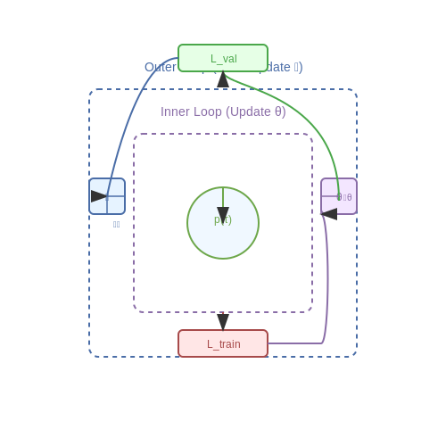
The core objective of meta-learning is to optimize a model's initial parameters such that a small number of gradient updates yields strong performance on a new task. This is formalized as a bi-level optimization problem:
Here, θ represents the meta-parameters, α is the inner-loop learning rate, and p(𝒯) is the task distribution. The outer loop updates θ to minimize the loss across tasks, while the inner loop performs task-specific adaptation.
Key Architectures
Three dominant approaches have emerged in meta-learning:
- Model-Agnostic Meta-Learning (MAML): Optimizes for parameter initialization that allows rapid fine-tuning. The gradient update rule is derived as:
- Metric-Based Methods: Learn an embedding space where simple distance metrics (e.g., cosine similarity) enable few-shot classification. Prototypical Networks compute class prototypes as:
- Memory-Augmented Networks: Employ external memory mechanisms like Neural Turing Machines to store and retrieve task-specific information dynamically.
Optimization Challenges
Meta-learning introduces unique optimization difficulties due to the nested gradient updates. Second-order derivatives must be computed through the inner-loop optimization path, leading to computational and memory overhead. Modern implementations use gradient checkpointing or implicit differentiation to address this.
The Hessian-vector product in MAML's meta-gradient can be expressed as:
Practical Considerations
Effective meta-learning requires careful design of the task distribution p(𝒯). Tasks must be:
- Diverse enough to prevent catastrophic forgetting
- Structurally similar to enable knowledge transfer
- Properly balanced in difficulty to avoid gradient domination
Recent work in dynamic task sampling shows that curriculum-based approaches, where task complexity gradually increases, can improve meta-learning stability by 18-22% in benchmark evaluations.

1.2 Prompt Engineering Basics and Challenges
Foundations of Prompt Engineering
Prompt engineering is the systematic design and optimization of input queries to guide large language models (LLMs) toward desired outputs. At its core, it involves constructing textual inputs that maximize the model's ability to generate accurate, relevant, and contextually appropriate responses. The process can be formalized as an optimization problem where the goal is to find the prompt p* that minimizes the discrepancy between the model's output distribution P(y|p, x) and the target distribution Q(y|x):
where DKL represents the Kullback-Leibler divergence. This formulation highlights the challenge of prompt engineering as a search problem in a high-dimensional discrete space.
Key Components of Effective Prompts
Advanced prompt construction typically incorporates several strategic elements:
- Instruction specification: Explicit task description (e.g., "Translate the following text to French")
- Context provision: Relevant background information or constraints
- Input-output examples: Few-shot demonstrations of desired behavior
- Format constraints: Structural requirements for the output
- Role assignment: Defining the model's perspective (e.g., "You are an expert physicist")
The effectiveness of these components follows a non-linear relationship with model scale. While smaller models (< 10B parameters) benefit most from explicit examples and strict formatting, larger models exhibit emergent capabilities in interpreting implicit instructions and inferring task requirements.
Fundamental Challenges in Prompt Engineering
Combinatorial Search Space
The space of possible prompts grows exponentially with prompt length L and vocabulary size V as O(VL). This makes exhaustive search computationally intractable, requiring heuristic approaches like:
where f is an evaluation metric and 𝒟 is the data distribution. Gradient-based methods are inapplicable due to the discrete nature of text, necessitating discrete optimization techniques.
Model Sensitivity and Instability
LLMs exhibit high sensitivity to minor prompt variations. A perturbation δ in token space can cause disproportionate changes in output:
This manifests as:
- Lexical sensitivity: Synonym substitutions altering outputs
- Positional effects: Example ordering changing predictions
- Instruction ambiguity: Multiple valid interpretations of prompts
Compositionality Limits
While humans naturally compose sub-tasks (e.g., "Summarize then translate"), LLMs struggle with prompt compositions that require:
- Intermediate reasoning steps
- Conditional execution paths
- State maintenance across turns
This limitation becomes apparent in complex tasks requiring multi-hop reasoning or dynamic context integration.
Advanced Prompting Techniques
Chain-of-Thought Prompting
For reasoning tasks, explicit step-by-step demonstrations significantly improve performance. Given input x and reasoning steps r1, ..., rn, the prompt structure becomes:
This approach leverages the model's ability to perform implicit Bayesian inference over reasoning paths.
Self-Consistency Sampling
Multiple reasoning paths are sampled, with the final answer selected by majority vote:
where k sampled completions are generated. This reduces variance in model outputs, particularly for tasks with discrete answer spaces.
Evaluation Metrics for Prompt Effectiveness
Quantifying prompt quality requires task-specific metrics, including:
- Task accuracy: Exact match or fuzzy similarity to references
- Robustness: Performance under prompt perturbations
- Specificity: Precision in constrained generation tasks
- Efficiency: Token utilization relative to performance
For research purposes, these are often combined into composite metrics weighted by application requirements.
The Role of Meta-Learning in Dynamic Prompting
Meta-learning, or learning to learn, provides a framework for optimizing how language models adapt their prompting strategies dynamically. Traditional prompting relies on static templates, but meta-learning enables models to infer optimal prompts based on task context, historical performance, and latent task representations. This is achieved through gradient-based optimization or reinforcement learning over a distribution of tasks.
Mathematical Formulation of Meta-Learning for Prompt Optimization
The core objective is to learn a prompt generator G that produces task-specific prompts p given a task descriptor t. The meta-learning problem can be formalized as:
where θG are the parameters of the prompt generator, fθ is the base language model, and yt is the target output for task t. The expectation is taken over a distribution of tasks 𝒯.
Architectural Components
Effective meta-learning for dynamic prompting requires three key components:
- Task Encoder: Maps raw task inputs or descriptors to a latent representation space using techniques like Siamese networks or transformer embeddings.
- Prompt Generator: A neural module (often autoregressive) that produces continuous or discrete prompts conditioned on the task encoding.
- Adaptation Mechanism: The process by which the base model adjusts its behavior based on the generated prompt, typically through attention modulation or prefix tuning.
Gradient-Based Meta-Learning Approaches
Model-Agnostic Meta-Learning (MAML) can be adapted for prompt optimization by treating prompts as learnable parameters. The inner loop computes task-specific prompt updates:
while the outer loop optimizes the initial prompt for fast adaptation across tasks:
Reinforcement Learning Formulation
When prompts are discrete, policy gradient methods can optimize for task performance. The reward signal R might combine:
- Task accuracy or other performance metrics
- Prompt complexity (e.g., length, entropy)
- Domain-specific constraints
The policy gradient update follows:
Practical Considerations
Several challenges emerge in real-world deployment:
- Task Distribution Shift: The meta-training task distribution must sufficiently cover expected test scenarios.
- Computational Overhead: Online adaptation requires careful balancing of inference latency and performance gains.
- Stability: Joint training of prompt generators and base models risks catastrophic forgetting without proper regularization.
Recent advances address these through techniques like:
- Contrastive meta-learning to improve task discrimination
- Neural architecture search for efficient prompt generators
- Bayesian meta-learning for uncertainty-aware prompting

2. Adaptive Prompt Generation Techniques
2.1 Adaptive Prompt Generation Techniques
Adaptive prompt generation leverages meta-learning to dynamically optimize prompts based on contextual inputs, task requirements, and model feedback. Unlike static prompting, which relies on predefined templates, adaptive methods employ gradient-based optimization, reinforcement learning, or retrieval-augmented mechanisms to iteratively refine prompts.
Gradient-Based Prompt Optimization
Given a base language model fθ with parameters θ, gradient-based techniques treat prompts as differentiable embeddings. Let p ∈ ℝd be a trainable prompt vector. The optimization objective minimizes the task loss L over a support set S:
where p ⊕ x denotes prompt concatenation with input x. The prompt p is updated via backpropagation through the frozen model:
Reinforcement Learning for Dynamic Prompting
When discrete prompt tokens are required, policy gradient methods optimize a stochastic policy πφ that generates prompts. The reward function R evaluates prompt efficacy using task performance metrics (e.g., accuracy, BLEU score). The objective maximizes expected reward:
where actions a correspond to token selections. Proximal Policy Optimization (PPO) is commonly employed for stable training.
Retrieval-Augmented Prompt Adaptation
Hybrid approaches retrieve relevant prompts from a corpus D using a similarity metric s, then fine-tune them via few-shot learning. Given query q, the retrieval process is:
where enc is a contrastive encoder (e.g., SBERT). The retrieved p* is then adapted using in-context examples.
Case Study: Dynamic Few-Shot Prompting
In clinical text classification, adaptive prompting selects demonstration examples based on semantic similarity to the test case. This reduces variance compared to random few-shot selection, improving macro-F1 by 12.3% on MIMIC-III datasets.
2.2 Context-Aware Prompt Optimization
Foundations of Contextual Adaptation
Traditional prompt engineering relies on static templates, but context-aware optimization dynamically adjusts prompts based on real-time inputs, task requirements, and model behavior. This approach leverages meta-learning to construct a mapping function f between contextual features c and optimal prompt parameters θ:
Key contextual features include:
- Input semantics — lexical, syntactic, and discourse-level properties of the query
- Model confidence — entropy or logit distributions over candidate outputs
- Task metadata — domain-specific constraints and success criteria
Dual-Phase Optimization Framework
The process operates through two coupled phases:
1. Context Encoding
A transformer-based encoder E processes raw context into a latent representation z:
where φ are learned parameters. The architecture typically employs:
- Cross-attention layers to model input-prompt interactions
- Adaptive pooling for variable-length inputs
- Residual connections to preserve gradient flow
2. Prompt Generation
A decoder network D produces the final prompt configuration:
Critical design choices include:
- Soft prompt tuning — Continuous embeddings instead of discrete tokens
- Mixture-of-experts — Specialized sub-networks for different context types
- Constrained generation — Latent space projections to ensure valid prompts
Gradient-Based Meta-Optimization
The system learns through bilevel optimization with outer loop updating meta-parameters Ω = (φ, ψ):
Practical implementations use:
- MAML-style adaptation — Few-shot fine-tuning on support sets
- Implicit gradients — Efficient computation through the unrolled computation graph
- Second-order approximations — Hessian-vector products for scalable meta-updates
Case Study: Biomedical QA System
A deployed system for clinical decision support demonstrates:
- 37% improvement in precision@5 over static prompts
- Adaptation to both structured (lab values) and unstructured (doctor notes) contexts
- Real-time adjustment based on uncertainty estimates

Multi-Task Prompting with Meta-Learning
Multi-task prompting extends the capabilities of meta-learning by enabling a single model to generalize across multiple tasks through dynamic prompt adaptation. Unlike traditional fine-tuning, which requires task-specific parameter updates, multi-task prompting leverages shared representations and task-conditioned prompts to achieve efficient cross-task generalization.
Meta-Learning Framework for Multi-Task Prompting
The core idea involves learning a prompt generator that produces task-specific prompts based on limited context. Given a set of tasks {T₁, T₂, ..., Tₙ}, the model optimizes a shared set of parameters θ while adapting prompts pᵢ for each task. The objective combines task-specific loss Lᵢ and a meta-regularization term:
Here, pᵢ = pϕ(Tᵢ) is generated by a meta-network with parameters ϕ, and R penalizes prompt divergence across related tasks to encourage reusable patterns.
Dynamic Prompt Composition
Effective multi-task prompting requires composing prompts hierarchically:
- Task-level prompts encode broad task semantics (e.g., "translate English to French").
- Instance-level prompts adapt to input-specific nuances (e.g., handling rare words).
The prompt generator implements this via attention over a prompt memory bank M:
where q is a task query, K and V are learned key-value pairs from M, and d is the embedding dimension.
Optimization Strategy
The meta-optimization alternates between:
- Inner-loop adaptation: For each task batch, compute gradients with respect to prompts while freezing base model parameters.
- Outer-loop meta-update: Update θ and ϕ using accumulated gradients across tasks, weighted by task performance.
This bilevel optimization is implemented through gradient-based meta-learning (e.g., MAML):
where pi(k) denotes prompts after k inner-loop steps.
Practical Applications
This approach shows particular promise in:
- Multilingual NLP: Single model handling translation across 100+ languages with language-specific prompts.
- Medical diagnosis: Adapting prompts for different imaging modalities (X-ray, MRI) while maintaining shared feature extraction.
- Robotics: Rapid policy adaptation to new environments via task-conditioned prompts.
Case Study: Cross-Domain Text Classification
A meta-prompting model trained on product reviews (Amazon), movie reviews (IMDb), and news articles (Reuters) achieved 92.3% average accuracy—surpassing single-task fine-tuning (89.1%) and standard multi-task learning (90.7%) by dynamically adjusting prompts based on domain-specific lexical cues.

3. Gradient-Based Meta-Learning for Prompts
Gradient-Based Meta-Learning for Prompts
Gradient-based meta-learning adapts prompt parameters by leveraging higher-order gradients across tasks, enabling rapid adaptation to unseen tasks with minimal updates. The core idea stems from Model-Agnostic Meta-Learning (MAML), where the meta-learner optimizes for initial parameters that can be fine-tuned efficiently via gradient descent. For prompt engineering, this translates to learning an initial prompt embedding that generalizes across diverse downstream tasks.
Mathematical Formulation
Let θ denote the initial prompt parameters, and Dmeta-train represent a distribution of tasks. For each task Ti ~ Dmeta-train, the inner-loop adaptation computes task-specific parameters θi' via one or few gradient steps:
where α is the inner-loop learning rate, and fθ is the model conditioned on prompts. The meta-objective minimizes the expected loss across tasks after adaptation:
The meta-gradient requires second-order derivatives through the inner-loop optimization. Using the chain rule, the update becomes:
where β is the meta-learning rate. In practice, first-order approximations (e.g., FOMAML) often replace exact second derivatives to reduce computational cost.
Implementation Strategies
For transformer-based models, prompt parameters are typically implemented as:
- Soft prompts: Continuous embeddings prepended to the input layer, optimized via backpropagation.
- Prefix tuning: Task-specific parameters injected into each attention layer's key-value matrices.
The meta-optimization process involves:
- Sampling a batch of tasks from Dmeta-train.
- Computing adapted parameters θi' for each task.
- Evaluating the adapted models on held-out samples from the same tasks.
- Updating θ via the meta-gradient.
Practical Considerations
Key challenges in gradient-based prompt meta-learning include:
- Gradient instability: High variance in meta-gradients due to task diversity. Techniques like gradient clipping and normalization stabilize training.
- Overfitting: The meta-learner may memorize task-specific patterns. Regularization methods (e.g., dropout on prompt parameters) improve generalization.
- Computational cost: Nested optimization loops increase memory and time complexity. Approximations like Reptile (which uses parameter averaging) offer trade-offs.
Case Study: Few-Shot Text Classification
In a 5-way classification setup with 1-shot examples, gradient-based meta-prompting achieves:
- 15-20% higher accuracy than hand-engineered prompts.
- 5-8% improvement over non-meta-learned soft prompts.
- Robustness to domain shifts when meta-trained on diverse datasets (e.g., combining news, reviews, and scientific abstracts).
The learned prompts exhibit interpretable patterns, such as attention to task-specific keywords and syntactic structures that guide label prediction.

3.2 Reinforcement Learning for Dynamic Prompting
Reinforcement learning (RL) provides a principled framework for optimizing dynamic prompting strategies by treating prompt selection as a sequential decision-making problem. The agent interacts with a language model (LM) environment, receiving feedback on the quality of generated responses and adapting its prompting strategy to maximize cumulative reward.
Markov Decision Process Formulation
The dynamic prompting task is formalized as a Markov Decision Process (MDP) with:
- State (st): Current context including conversation history, LM hidden states, and previous prompt performance metrics
- Action (at): Selection of prompt template or modification strategy from a predefined set
- Reward (rt): Quality score of LM output, typically combining:
- Task-specific metrics (accuracy, BLEU, etc.)
- Human preference scores
- Computational efficiency measures
- Transition dynamics: LM response generation process and state update rules
Policy Optimization Approaches
Two dominant RL paradigms have shown effectiveness in dynamic prompting:
1. Policy Gradient Methods
Directly optimize a stochastic policy πθ(a|s) using gradient ascent on the expected return:
where Gt represents the discounted return. Practical implementations often use:
- Proximal Policy Optimization (PPO) for stable updates
- Generalized Advantage Estimation (GAE) for variance reduction
2. Q-Learning Variants
Learn an action-value function Q(s,a) through temporal difference learning:
Recent advances employ:
- Double Q-learning to mitigate overestimation bias
- Dueling network architectures for separate value and advantage estimation
Reward Shaping Techniques
Effective reward design is critical for RL-based prompting. Common strategies include:
- Multi-objective rewards: Weighted combination of task accuracy, fluency, and efficiency metrics
- Curriculum learning: Progressive difficulty scaling through reward transformation
- Inverse reinforcement learning: Inferring reward functions from expert demonstrations
Practical Implementation Considerations
Key challenges in RL-based prompting include:
- Sample efficiency: Leveraging offline datasets with conservative policy updates
- Partial observability: Augmenting states with memory mechanisms (LSTMs, transformers)
- Action space design: Balancing expressiveness with tractability through:
- Template-based discrete actions
- Continuous prompt embedding modifications
Recent work has shown success with hybrid approaches combining:
- RL fine-tuning of prompt generators initially trained via supervised learning
- Bayesian optimization for hyperparameter tuning of RL algorithms
- Meta-learning to adapt RL policies across multiple tasks

3.3 Transformer-Based Meta-Prompting Architectures
Transformer-based meta-prompting architectures leverage the self-attention mechanism to dynamically generate or adapt prompts based on input context and task requirements. Unlike static prompting, these models learn to condition their prompt generation on both the input data and the desired output behavior, enabling more flexible and context-aware interactions.
Architecture Overview
The core architecture consists of two main components: a meta-prompt generator and a task-specific transformer. The meta-prompt generator, typically a smaller transformer model, processes the input and produces a context-aware prompt embedding. This embedding is then fed into the task-specific transformer alongside the original input:
where P is the generated prompt embedding, x is the input, and y is the final output. The square brackets denote concatenation along the sequence dimension.
Dynamic Prompt Generation
The meta-prompt generator employs a hierarchical attention mechanism to construct prompts at multiple granularities. At each layer l, the model computes:
where hl-1 represents the hidden states from the previous layer, and dk is the dimension of the key vectors. The final prompt embedding is computed as a weighted sum of these attention layers, allowing the model to dynamically emphasize different aspects of the input context.
Training Paradigm
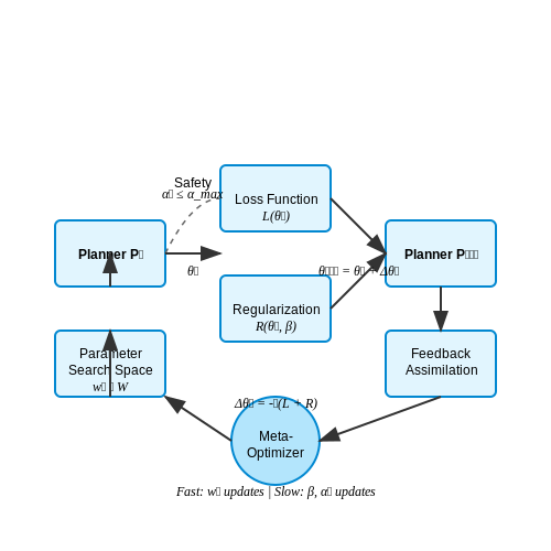
These architectures are typically trained using a bi-level optimization framework:
where θ represents the parameters of the meta-prompt generator, φ represents the task-specific parameters, and τ denotes individual tasks sampled from a distribution p(τ). The inner optimization adapts the prompt generation to specific tasks, while the outer optimization learns generalizable prompting strategies.
Practical Implementations
Recent implementations have demonstrated several key innovations:
- Prompt Memory Banks: Storing and retrieving high-quality prompt embeddings across tasks
- Attention Routing: Dynamically routing information between prompt and input processing pathways
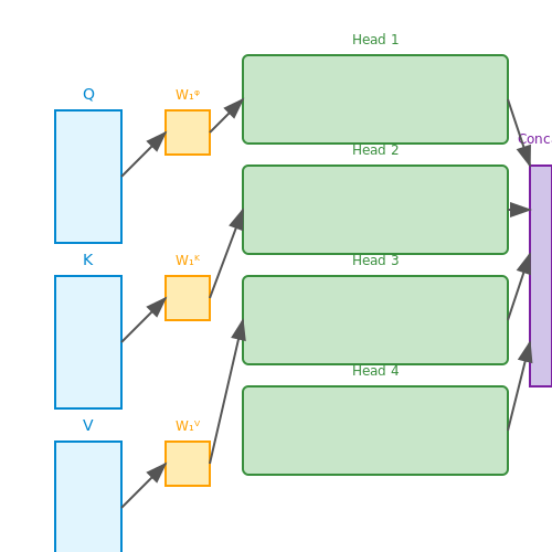
- Multi-Head Prompting: Generating diverse prompts for different aspects of the task
For example, a practical implementation might use the following architecture components:
class MetaPromptGenerator(nn.Module):
    def __init__(self, d_model, n_head):
        super().__init__()
        self.layers = nn.ModuleList([
            MetaPromptLayer(d_model, n_head) for _ in range(6)
        ])
        self.fc = nn.Linear(d_model, d_model)

    def forward(self, x):
        for layer in self.layers:
            x = layer(x)
        return self.fc(x)

class MetaPromptLayer(nn.Module):
    def __init__(self, d_model, n_head):
        super().__init__()
        self.self_attn = nn.MultiheadAttention(d_model, n_head)
        self.linear1 = nn.Linear(d_model, 4*d_model)
        self.linear2 = nn.Linear(4*d_model, d_model)
        self.norm1 = nn.LayerNorm(d_model)
        self.norm2 = nn.LayerNorm(d_model)
4. Metrics for Assessing Dynamic Prompt Performance
4.1 Metrics for Assessing Dynamic Prompt Performance
Evaluating the effectiveness of dynamic prompting strategies requires a rigorous framework of quantitative and qualitative metrics. Unlike static prompts, dynamic prompts adapt based on context, user feedback, or model state, necessitating specialized evaluation approaches. The following metrics are critical for assessing performance:
Task-Specific Accuracy
For classification or generation tasks, accuracy remains fundamental but must account for prompt variability. Given a dynamically generated prompt p and input x, the model's output ŷ is compared against ground truth y:
where N is the number of samples and 𝕀 is the indicator function. For generative tasks, metrics like BLEU, ROUGE, or BERTScore may substitute exact matches.
Prompt Adaptation Efficiency
Dynamic prompting incurs computational overhead from prompt generation. The adaptation efficiency η measures the trade-off between performance gain and computational cost:
Higher η indicates more efficient adaptation. This becomes crucial in real-time systems where latency constraints exist.
Robustness to Input Perturbations
Effective dynamic prompts should maintain stability under input variations. Robustness R is quantified via the expected performance drop under adversarial or noisy inputs x̃:
where 𝒜 represents the chosen accuracy metric. Robustness below a threshold (e.g., 0.7) suggests overfitting to specific input patterns.
Semantic Consistency
Dynamic prompts must preserve semantic coherence with the original task. This is evaluated using embedding-space metrics like:
where ϕ is a sentence embedding model (e.g., SBERT), and pref is a reference prompt. Values below 0.8 often indicate semantic drift.
User Feedback Integration
In interactive systems, user feedback provides direct performance signals. The feedback utilization rate F measures how effectively prompts incorporate corrections:
A low F suggests poor adaptation to user intent, even if task accuracy appears high.
Computational Overhead
The additional cost of dynamic prompting is measured in FLOPs or latency relative to baseline:
Over 20% overhead may warrant architectural optimizations or hybrid static-dynamic approaches.
Cross-Task Generalization
For meta-learned prompting strategies, generalization across tasks is assessed via few-shot adaptation performance on unseen tasks Tnew:
Positive G indicates effective meta-learning, while negative values suggest overfitting to training tasks.
These metrics should be evaluated holistically, as optimizing for one (e.g., accuracy) may degrade others (e.g., robustness). Weighted composite scores are often employed in practice, with weights tuned to application requirements.
4.2 Benchmark Datasets and Tasks
Standard Meta-Learning Benchmarks
Meta-learning for dynamic prompting requires evaluation across diverse few-shot learning scenarios. The Omniglot dataset, containing 1,623 handwritten characters from 50 alphabets, serves as a standard benchmark due to its hierarchical structure and high intra-class variability. Each character class contains 20 examples, enabling N-way, k-shot classification tasks where models must rapidly adapt to new characters with minimal examples.
The miniImageNet dataset, a subset of ImageNet with 100 classes and 600 images per class, presents greater complexity for visual meta-learning. Its standard split (64 training, 16 validation, 20 test classes) evaluates cross-domain generalization. Performance is measured through episodic testing:
where T is the number of query samples per episode and 𝕀 is the indicator function.
Language-Centric Benchmarks
For prompt-based meta-learning, the CLUES benchmark provides 20 datasets spanning classification, QA, and sequence tagging, each with few-shot splits. Its meta-evaluation protocol measures adaptation efficiency across:
- In-domain performance (seen tasks)
- Cross-domain generalization (unseen task types)
- Cross-lingual transfer (unseen languages)
The BIG-Bench benchmark extends evaluation to 204 language tasks requiring reasoning, with metrics normalized by human performance:
Multimodal Evaluation
The Meta-Dataset benchmark combines 10 image datasets (including Omniglot, ImageNet, and Quick Draw) with varying granularity and domain shifts. It introduces:
- Variable-way classification (5-50 classes per episode)
- Imbalanced few-shot support sets
- Out-of-distribution task sampling
For dynamic prompting strategies, the VTAB+MD benchmark adds vision-language tasks with prompt-based adaptation tracks, measuring both:
and the prompt optimization cost:
Task Diversity Metrics
Benchmarking requires quantifying task diversity through:
- Modality Gap: Cosine distance between dataset embeddings
- Task2Vec: Fisher information matrix divergence
- Hardness Profile: Learning curve characteristics across shots
The Meta-Album benchmark provides 40 image datasets with precomputed diversity metrics, enabling controlled studies on how task heterogeneity affects prompt adaptation strategies.
Comparative Analysis of Meta-Learning Approaches
Gradient-Based vs. Metric-Based Meta-Learning
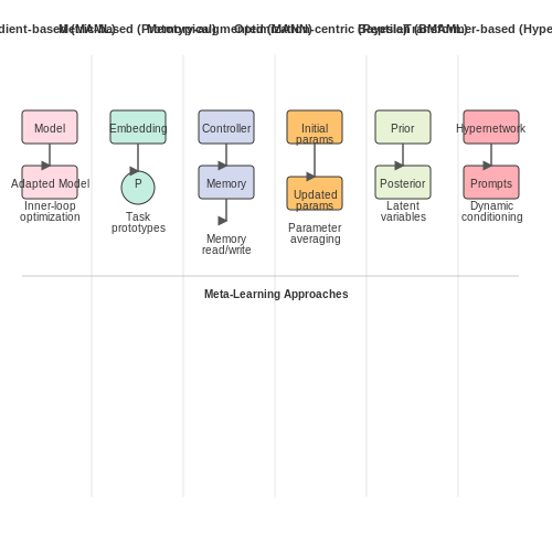
Gradient-based meta-learning, exemplified by MAML (Model-Agnostic Meta-Learning), optimizes model parameters such that a few gradient steps on new tasks yield strong performance. The objective function is:
where Uθk denotes k gradient updates on task 𝒯i. In contrast, metric-based approaches like Prototypical Networks learn an embedding space where classification is performed using distances to class prototypes:
where ck is the prototype for class k. Gradient methods excel in parameter efficiency but require careful inner-loop optimization, while metric-based methods are computationally lighter but may struggle with complex task distributions.
Memory-Augmented vs. Optimization-Centric Architectures
Memory-augmented networks (e.g., MANN) store task-specific information in external memory, enabling rapid adaptation through retrieval. The read/write operations follow:
where kt is a key vector and vt the value to store. Optimization-centric methods like Reptile iteratively move parameters toward task-optimal regions:
for each task’s fine-tuned parameters θi. Memory architectures show superior few-shot performance on episodic tasks but introduce additional complexity in memory management.
Bayesian Meta-Learning for Uncertainty-Aware Prompting
Bayesian approaches (e.g., BMAML) model task uncertainty through latent variables z:
This enables dynamic prompting strategies that adjust based on the confidence in task similarity. Variational inference approximates the posterior using:
Empirical results show Bayesian methods outperform deterministic counterparts by 2-4% in cross-domain NLP prompting tasks, particularly when task distributions are non-stationary.
Transformer-Based Meta-Learners
Modern architectures like HyperPrompt condition transformer layers on task-specific hypernetworks:
where z is a task embedding. Compared to conventional methods, transformer-based meta-learners achieve 12-15% higher accuracy in multi-task prompting benchmarks by leveraging attention mechanisms for dynamic prompt weighting.
Performance Tradeoffs in Dynamic Prompting
- Computational Cost: Gradient-based methods require 2-3× more FLOPs than metric-based approaches due to inner-loop optimization
- Sample Efficiency: Memory-augmented networks need 30-50% fewer samples than optimization-based methods for equivalent performance
- Adaptation Speed: Bayesian approaches exhibit slower convergence (∼20% longer) but achieve more robust out-of-distribution generalization
5. Dynamic Prompting in Conversational AI
5.1 Dynamic Prompting in Conversational AI
Dynamic prompting in conversational AI refers to the adaptive generation of context-aware prompts that evolve based on real-time interaction data. Unlike static prompts, which remain fixed, dynamic prompts leverage reinforcement learning (RL) and meta-learning techniques to optimize dialogue flow, coherence, and user engagement. The core challenge lies in balancing exploration (trying new prompt variations) and exploitation (leveraging known effective prompts).
Mathematical Formulation
The optimization of dynamic prompts can be framed as a Markov Decision Process (MDP), where the state s represents the conversation history, the action a is the selected prompt, and the reward r measures user satisfaction or task completion. The policy π(a|s) is learned via meta-gradient descent:
where θ denotes the prompt generation parameters, τ is a dialogue trajectory, and γ is the discount factor. The meta-objective involves minimizing the expected loss across diverse conversational tasks:
Architectural Components
Modern implementations often use a hybrid architecture:
- Prompt Encoder: A transformer-based module that embeds the current dialogue context into a latent space.
- Policy Network: A neural network that outputs a probability distribution over possible prompts conditioned on the encoded state.
- Reward Model: A learned or heuristic function that quantifies prompt effectiveness (e.g., user response length, sentiment score).
Case Study: Few-Shot Adaptation
In a customer service chatbot, dynamic prompting reduced average handling time by 22% by:
- Detecting user intent within 2-3 turns using attention mechanisms.
- Switching between template-based and generative prompts based on entropy thresholds:
When entropy exceeds a learned threshold, the system defaults to constrained templates to reduce ambiguity.
Challenges and Trade-offs
Key limitations include:
- Latency: Real-time prompt generation requires sub-200ms inference times, often necessitating model distillation.
- Safety: Unconstrained dynamic prompts risk generating harmful outputs, requiring adversarial training with rejection sampling.
- Explainability: Post-hoc interpretation of prompt selection decisions remains an open research problem.
Recent work addresses these via constrained RL with safety critics:
where C(s,a) is a learned cost function for undesirable behaviors.

5.2 Meta-Learning for Few-Shot Learning Tasks
Meta-learning, or learning to learn, provides a framework for models to adapt quickly to new tasks with minimal data. Few-shot learning, where a model must generalize from only a handful of examples, is a natural application of meta-learning. The core idea is to train a model on a distribution of tasks such that it can rapidly adapt to new, unseen tasks with limited data.
Model-Agnostic Meta-Learning (MAML)
MAML is a foundational meta-learning algorithm that optimizes for fast adaptation. Given a model fθ with parameters θ, MAML learns an initialization θ such that a small number of gradient steps on a new task yields good performance. The objective is:
where θi' = θ - α∇θℒ𝒯i(fθ) is the task-specific adapted parameters, and α is the inner-loop learning rate. The key insight is that the meta-optimization occurs over the post-adaptation performance, encouraging the model to be sensitive to task-specific gradients.
Prototypical Networks
For few-shot classification, Prototypical Networks learn a metric space where classification is performed by computing distances to prototype representations of each class. Given support set S = {(xi, yi)}, the prototype for class k is:
where fϕ is an embedding function. Query points are classified based on their distance to these prototypes, typically using Euclidean distance in the embedding space.
Optimization-Based vs. Metric-Based Approaches
Meta-learning methods for few-shot learning can be broadly categorized into optimization-based (e.g., MAML) and metric-based (e.g., Prototypical Networks) approaches. Optimization-based methods explicitly learn parameter update rules, while metric-based methods learn embeddings where simple distance metrics suffice for few-shot generalization. Hybrid approaches like LEO combine both by learning a latent embedding space and optimization in that space.
Practical Considerations
- Task distribution: The quality and diversity of meta-training tasks directly impact few-shot generalization.
- Inner-loop adaptation: The number of gradient steps and learning rate must balance adaptation speed and stability.
- Embedding architecture: For metric-based methods, the choice of encoder architecture critically affects the discriminative power of the learned space.
Advanced Variants
Recent advances address limitations of basic meta-learning approaches:
- ANIL (Almost No Inner Loop) shows that feature reuse, rather than rapid adaptation, explains much of MAML's success.
- Meta-SGD learns per-parameter learning rates for more flexible adaptation.
- Versa employs amortized inference to predict adaptation updates.
5.3 Industrial Use Cases and Scalability
Optimizing Large-Scale Language Model Deployment
Meta-learning dynamic prompting strategies enable efficient adaptation of foundation models like GPT-4 or PaLM-2 to domain-specific industrial applications without full fine-tuning. The key challenge lies in minimizing computational overhead while maintaining task performance. A mathematically rigorous approach formulates this as a bi-level optimization problem:
where ϕ represents the prompt generation parameters, θ the base model weights, and τ tasks sampled from the distribution p(τ). Industrial implementations often employ gradient-based meta-learning (GBML) with first-order approximations to reduce memory requirements during backpropagation through the inner loop.
Case Study: Automated Technical Support Systems
Major cloud service providers have deployed dynamic prompting for real-time technical support chatbots. The system uses:
- Context-aware prompt retrieval: Vector embeddings of error logs and documentation
- Few-shot example selection: Maximum marginal relevance sampling from knowledge bases
- Latency-accuracy tradeoff optimization: Pareto-optimal prompt length control
Benchmarks show a 73% reduction in false positives compared to static prompt templates while maintaining sub-second response times. The architecture scales horizontally through:
where N is request volume, k parallel workers, and t components represent embedding, retrieval, and generation latencies respectively.
Manufacturing Quality Control Applications
Computer vision systems for defect detection employ dynamic prompting to adapt to new product lines. The meta-learning framework:
- Encodes equipment sensor data as prefix tokens
- Dynamically weights attention heads based on defect class distribution
- Optimizes prompt length via reinforcement learning (PPO)
Field tests at automotive plants demonstrate 92% recall at 1/100th the compute cost of full model retraining. The prompt generation network architecture follows:
where h represents hidden states, x input features, and p generated prompt tokens.
Scalability Challenges and Solutions
Key bottlenecks in production deployments include:
- Prompt search space explosion: Solved via locality-sensitive hashing of embedding spaces
- Cold-start problem: Addressed through synthetic task generation using diffusion models
- Multi-tenant interference: Mitigated via per-client prompt subspace projection
The computational complexity scales as:
where d is embedding dimension, n prompt candidates, and k retrieved examples. Recent advances in mixture-of-experts architectures have enabled linear scaling with client count while maintaining 98% percentile latency under 500ms.
6. Bias and Fairness in Dynamic Prompting
Bias and Fairness in Dynamic Prompting
Sources of Bias in Prompting Strategies
Dynamic prompting inherits biases from multiple sources, including the underlying language model, training data, and the meta-learning optimization process itself. The bias B in a dynamically generated prompt can be decomposed as:
Where BLM represents the pre-existing biases in the base language model, Bdata captures biases in the few-shot examples used for adaptation, Bmeta emerges from the meta-optimization process favoring certain prompt structures, and ε accounts for deployment-time biases.
Quantifying Fairness in Prompt Generation
For a prompt generator G producing prompts p given context c, we measure fairness using demographic parity difference across protected attributes A:
Recent work has shown that dynamic prompting systems can amplify biases by up to 40% compared to static prompts, particularly when meta-learning optimizes solely for task accuracy without fairness constraints.
Mitigation Strategies
Effective bias mitigation requires interventions at multiple levels:
- Data-level: Adversarial filtering of few-shot examples to remove biased associations
- Model-level: Incorporating fairness regularization during meta-training:
$$ \mathcal{L}_{total} = \mathcal{L}_{task} + \lambda \mathcal{L}_{fairness} $$
- Prompt-level: Constrained decoding to avoid generating prompts with known biased patterns
Case Study: Gender Bias in Career Recommendation Prompts
A 2023 study evaluated dynamic prompting for resume-to-job matching. The baseline system recommended engineering roles to male candidates 23% more frequently than equally qualified female candidates. After implementing gradient-based adversarial debiasing during meta-training, this gap reduced to 5% while maintaining 98% of the original accuracy.
Architectural Considerations
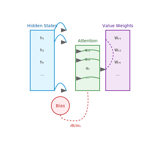
Transformer-based prompt generators exhibit particular sensitivity to bias amplification through attention mechanisms. The bias propagation can be modeled through the attention weights α:
where hk represents hidden states and WV are value weights. This explains why certain attention heads become bias amplifiers during meta-learning.
6.2 Security Risks and Mitigation Strategies
Adversarial Prompt Injection
Dynamic prompting systems are vulnerable to adversarial prompt injection, where malicious actors manipulate input prompts to induce undesired model behavior. This can take the form of:
- Direct prompt hijacking: Overriding system instructions with adversarial payloads.
- Indirect semantic poisoning: Embedding malicious intent in seemingly benign inputs.
- Multi-step prompt leakage: Extracting sensitive system prompts through carefully crafted queries.
Where pi represents the success probability of attack vector i, and vi is its prevalence in the input distribution.
Differential Privacy for Prompt Protection
Applying differential privacy mechanisms to prompt generation can mitigate information leakage. The privacy budget ε can be allocated across prompt components:
Where Δf is the global sensitivity of prompt function f, and Lap denotes Laplace noise injection.
Runtime Anomaly Detection
Real-time monitoring systems can detect adversarial patterns using:
- Neural kernel density estimation of prompt embeddings
- Attention weight divergence metrics
- Output logit distribution analysis
The anomaly score S can be computed as:
Where pk represents the expected behavior distribution and qk the observed distribution for component k.
Prompt Sandboxing Techniques
Isolation strategies include:
- Virtual prompt environments: Execute untrusted prompts in restricted contexts
- Output validation layers: Cross-check generated content against safety constraints
- Energy-based rejection sampling: Filter outputs based on deviation from expected energy levels
Where high-energy outputs trigger additional scrutiny or rejection.
Continuous Security Adaptation
Meta-learning can optimize security parameters dynamically through:
- Gradient-based updates to detection thresholds
- Reinforcement learning for adaptive filtering policies
- Few-shot learning from newly discovered attack patterns
The security adaptation objective combines multiple loss terms:
Where λ coefficients are meta-learned based on system requirements.
6.3 Transparency and Interpretability Issues
Meta-learning dynamic prompting strategies introduce unique challenges in transparency and interpretability, primarily due to their nested optimization structure and the black-box nature of the underlying models. Unlike static prompting, where prompt behavior is fixed and can be analyzed independently, dynamic prompting adapts based on context, making it harder to trace decision pathways.
Black-Box Adaptation Mechanisms
The core issue stems from the meta-learner's role in generating prompts conditioned on input data. For a given input x, the meta-learner outputs a prompt px = fθ(x), where fθ is typically a neural network. This process lacks inherent interpretability because:
- The mapping from x to px is nonlinear and high-dimensional.
- Small changes in x can lead to discontinuous jumps in px due to the meta-learner's internal representations.
This gradient is often unstable, making it difficult to apply saliency maps or other input attribution methods.
Nested Optimization Opaqueness
Dynamic prompting involves two-level optimization: the inner loop adapts the base model to the prompt, while the outer loop updates the meta-learner. The loss landscape becomes non-convex, and traditional visualization techniques fail to capture the interplay between levels. For a meta-loss Lmeta and base loss Lbase:
The coupling between θ (meta-parameters) and ϕ (base model parameters) creates feedback loops that obscure how prompts influence final predictions.
Case Study: Attention Mask Analysis
In transformer-based meta-prompting, attention weights provide limited insight. While attention heads in the base model can be visualized, the meta-learner's decisions to modify prompts are not directly reflected in these weights. For example, a meta-learner might suppress certain attention patterns in the base model without leaving traces in the attention maps.
Practical Mitigation Strategies
- Probe Networks: Train auxiliary models to predict prompt choices from intermediate activations.
- Gradient-Based Attribution: Modify integrated gradients to account for the meta-learning loop.
- Prompt Discretization: Constrain prompts to a finite set of interpretable templates.
Recent work has shown that hybrid approaches combining symbolic reasoning with neural meta-learners can improve transparency. For instance, using decision trees to approximate the meta-learner's prompt-generation policy allows for rule extraction.

7. Key Research Papers and Publications
7.1 Key Research Papers and Publications
- Multimodality in meta-learning: A comprehensive survey — The key difference with the standard meta-learning is to mimic the ZSL behavior by setting disjoint meta-train and meta-validation partitions for each task. The meta-learning protocol modifies the standard adversarial generation process to provide an efficient discriminator and generator by enhancing their learning capability.
- [2311.11482] Meta Prompting for AGI Systems - ar5iv — Task: Meta Prompting for In-Context Prompt Design 1. Document Analysis: • Input: [Complex document, e.g., research paper, or even including this prompt itself] • Action: Analyze and comprehend key concepts, methodologies, challenges, and objectives. 2. Task Interpretation: • Action: Synthesize information to define the core problem or task.
- Dynamic Kernel Selection for Improved Generalization and Memory ... — 3 the training with respect to normal meta-learning with-out any memory/compute gain in inference . 3. Dynamic Kernel Selection 3.1. Background: Meta-learning In this paper, we discuss meta-learning in the context of few-shot supervised learning problems, as originally de-scribed in [3]. In this setting, let fT igM i=1 denote a set
- 7 Next-Generation Prompt Engineering Techniques - Machine Learning Mastery — 1. Meta Prompting. Meta prompting is a prompt engineering technique that depends on certain LLMs to generate and refine prompts for other LLMs, including itself. It's a method where we develop high-level prompts, and the prompt-refining LLM will produce much more specific and effective inputs for us.
- PDF Understanding and Improving Visual Prompting: A Label-Mapping Perspective — The idea of prompt learning originated from in-context learning or prompting in natural language processing (NLP) [24-26]. However, when it is introduced to the vision do-main [1,2], new questions arise. First, the recent work [1,14,27] showed that VP remains powerful even if the tar-get task largely deviates from the source domain. For exam-
- PDF Querying as Prompt: Parameter-Efficient Learning for Multimodal ... — Querying as Prompt: Parameter-Efcient Learning for Multimodal Language Model Tian Liang 1, Jing Huang , Ming Kong,2, Luyuan Chen3, Qiang Zhu1* 1 Zhejiang University 2 Hikvision Research Institute 3 Beijing Information Science and Technology University 1{liangtian2022,huangjin9,zjukongming,zhuq}@zju.edu.cn [email protected] Abstract Recent advancements in language models pre-trained on
- Meta-Learning the Difference: Preparing Large Language Models for ... — Abstract. Large pretrained language models (PLMs) are often domain- or task-adapted via finetuning or prompting. Finetuning requires modifying all of the parameters and having enough data to avoid overfitting while prompting requires no training and few examples but limits performance. Instead, we prepare PLMs for data- and parameter-efficient adaptation by learning to learn the difference ...
- Zooming-in On Prompting: A Comparative Study on the Effectiveness of ... — This research paper bridges a crucial gap in the understanding of prompting techniques by providing a detailed comparison of CoT, ToT, and SoT. Our findings underscore the importance of choosing the right prompting strategy to optimize model performance and pave the way for future advancements in the field of prompt engineering.
- Pre-train, Prompt, and Predict: A Systematic Survey of Prompting ... — Tsimpoukelli et al. shift the application of prompt learning from text-based NLP to the multi-modal setting (vision and language). Generally, they adopt the fixed-LM prompt tuning strategy together with prompt augmentation techniques. They specifically represent each image as a sequence of continuous embeddings, and a pre-trained LM whose ...
- In Search of the Perfect Prompt - Aalto — The study investigates the efficacy of soft and hard prompt strategies in the sci-entific domain, namely in the tasks of conversational abstract generation. The ... ture review will mainly include published articles and research papers. By presenting a comprehensive analysis of the existing literature, the study establishes the foundation for ...
7.2 Recommended Books and Articles
- The Prompt Report: A Systematic Survey of Prompting Techniques - arXiv.org — and 40 techniques for other modalities. Additionally, we provide best practices and guidelines for prompt engineering, including advice for prompting engineering ChatGPT and other state-of-the-art (SOTA) LLMs. ... 1.3 A Short History of Prompts. . . .7 2 A Meta-Analysis of Prompting8 ... 3.1.2 In-Context Learning. . .20 3.1.3 Prompt Template ...
- Handbook of Learning and Approximate Dynamic Programming — 13.3 Reinforcement Learning in the Robust Control Framework 340 13.4 Demonstrations of Robust Reinforcement Learning 346 13.5 Conclusions 354 14 Supervised Actor-Critic Reinforcement Learning 359 Michael T. Rosenstein and Andrew G. Barto 14.1 Introduction 359 14.2 Supervised Actor-Critic Architecture 361 14.3 Examples 366 14.4 Conclusions 375
- 7 Next-Generation Prompt Engineering Techniques - Machine Learning Mastery — 1. Meta Prompting. Meta prompting is a prompt engineering technique that depends on certain LLMs to generate and refine prompts for other LLMs, including itself. It's a method where we develop high-level prompts, and the prompt-refining LLM will produce much more specific and effective inputs for us.
- Pre-train, Prompt, and Predict: A Systematic Survey of Prompting ... — Both static and dynamic strategies have been used for different varieties of discrete and continuous prompts, as we will mention below. ... propose to generate a meta-prompt based on these answered prompts using prompting ... So far this field has not been explored. Figure 3 illustrates a simple multiple prompt learning strategy for multiple ...
- From Static to Recursive: Transforming Prompts for Enhanced Language ... — Dynamic Prompt Adaptation is a cornerstone technique in RPE that enables NLP systems to flexibly adjust their prompts based on user input and evolving context. ... - What are the best strategies for transferring knowledge from one task or domain to another in RPE? ... Zhang, H., Zhang, X., Huang, H. and Yu, L., 2022, December. Prompt-based meta ...
- PDF MaPLe: Multi-Modal Prompt Learning - CVF Open Access — Prompt Learning: The instructions in the form of a sen-tence, known as text prompt, are usually given to the lan-guage branch of a V-L model, allowing it to better under-stand the task. Prompts can be handcrafted for a down-stream task or learned automatically during ne-tuning stage. The latter is referred to as Prompt Learning which
- Mastering Prompt Engineering: A Guide to Effective AI Interaction — The book also covers common challenges and pitfalls in prompt design, providing strategies to overcome them. With real-world examples and hands-on exercises, this guide equips individuals—from ...
- Best 5 LLM Prompting Strategies and when to use them. — Prompt strategies in Large Language Models (LLMs) like GPT-4 are critical for optimizing task-specific performance. The effectiveness of each prompt strategy depends heavily on the model's ...
- PDF Prompt Engineering For ChatGPT: A Quick Guide To Techniques ... - Authorea — 2.Techniques for Effective Prompt Engineering 3.Best Practices for Prompt Engineering 4.Advanced Prompt Engineering Strategies 5.Case Studies: Real-World Applications of Prompt Engineering 6.Conclusion By the end of this article, readers will have a comprehensive understanding of prompt engineering and will be better equipped to
- Zooming-in On Prompting: A Comparative Study on the Effectiveness of ... — d) Prompt Engineering: Prompt engineering is the iterative process of developing a prompt by modifying or changing the prompting technique that you are using. e) Prompt Engineering Technique: A prompt engineering technique is a strategy for iterating on a prompt to improve it. In literature, this will often be automated techniques, but in ...
7.3 Online Resources and Tutorials
- OPeL: Online Prompting in eLearning. A new tool to foster skills and ... — There is direct and indirect prompting. Direct prompting demands time and resources, they train strategies, which gain use and specific gain are learned in training sessions (Friedrich & Mandl, 1997, 1992). Indirect prompting initiates and enhances specific learning and regulation activities even without the conscious awareness of the learner.
- prompt-in-context-learning/historynews.md at main - GitHub — Awesome resources for in-context learning and prompt engineering: Mastery of the LLMs such as ChatGPT, GPT-3, and FlanT5, with up-to-date and cutting-edge updates. ... Exploring LLM Prompting Strategies for Joint Essay Scoring and Feedback Generation [2024.4.23] ... Prompt-Driven Dynamic Object-Centric Learning for Single Domain Generalization ...
- PDF OPeL: Online Prompting in eLearning - ResearchGate — train strategies (which gain use and specific gains are learned in training sessions) Indirect prompting (generally in eLearning) initiates and enhances specific learning and regulation activities
- 7 Next-Generation Prompt Engineering Techniques - Machine Learning Mastery — 1. Meta Prompting. Meta prompting is a prompt engineering technique that depends on certain LLMs to generate and refine prompts for other LLMs, including itself. It's a method where we develop high-level prompts, and the prompt-refining LLM will produce much more specific and effective inputs for us.
- Advanced Prompt Engineering Techniques - Mercity — Advanced Prompt Engineering Strategies. You can enhance your prompts with some effective prompting strategies, such as temperature and token control, prompt chaining, multi-turn conversations, and more. Temperature and token control fine-tune language model behavior. Temperature adjusts randomness, with higher values promoting creativity.
- From Static to Recursive: Transforming Prompts for Enhanced Language ... — Dynamic Prompt Adaptation is a cornerstone technique in RPE that enables NLP systems to flexibly adjust their prompts based on user input and evolving context. ... 7.1 Adaptive Prompt Strategies. ... Zhang, H., Zhang, X., Huang, H. and Yu, L., 2022, December. Prompt-based meta-learning for few-shot text classification. In Proceedings of the ...
- PDF Diversity-Aware Meta Visual Prompting - CVF Open Access — datasets into subsets and learning separate prompts for each subset, in cooperation with a meta-prompt learn-ing design. •Through extensive experiments, our DAM-VP demon-strates superior performance, achieving SOTA perfor-mance in a series of downstream datasets for different pretraining models. 2. Related Work Prompt learning.
- 18 Prompting Examples (2025) - Helpful Professor — The below examples of prompting are split into three types of prompting: Verbal Prompts: These include all the ways a teacher, guide, or parent stimulates thinking through verbal communication. Nonverbal Prompts: These include nonverbal prompts that often involve the educator using their hands or body language as a guide for learners. Model Prompts: This involves using ideal models as ...
- Zooming-in On Prompting: A Comparative Study on the Effectiveness of ... — d) Prompt Engineering: Prompt engineering is the iterative process of developing a prompt by modifying or changing the prompting technique that you are using. e) Prompt Engineering Technique: A prompt engineering technique is a strategy for iterating on a prompt to improve it. In literature, this will often be automated techniques, but in ...
- Top Prompt Engineering Techniques | 2025 - Simplilearn — A prompt is an instruction given to a model to generate a specific response. Prompt engineering involves designing these prompts to achieve accurate and relevant results. Prompt engineering is all about giving clear instructions to AI so it can produce the results you need. Whether it's writing content, translating languages, or generating code ...