Training Compact LLMs Without Performance Drop
1. Defining Compact LLMs: Parameters, Architecture, and Use Cases
Defining Compact LLMs: Parameters, Architecture, and Use Cases
Architectural Foundations of Compact LLMs
Compact large language models (LLMs) are characterized by their reduced parameter count while maintaining competitive performance. Architecturally, they inherit the transformer-based design of their larger counterparts but employ optimizations such as:
- Pruned attention heads: Reducing the number of attention heads in multi-head attention layers while preserving the most salient ones.
- Factorized embeddings: Decomposing the embedding matrix into smaller matrices to reduce memory footprint.
- Depth-wise separable convolutions: Replacing dense feedforward layers with more efficient operations.
The parameter efficiency can be quantified by examining the scaling laws of transformer models. For a standard transformer with L layers, d model dimension, and h attention heads, the total parameters scale as:
where V is the vocabulary size. Compact models typically reduce L, d, or both while maintaining the performance-to-parameter ratio.
Performance-Parameter Tradeoffs
The relationship between model size and performance follows a power-law distribution, as established by Kaplan et al. (2020):
where N is the number of parameters, Nc is a critical scale, and α ≈ 0.07 for language models. Compact LLMs operate in the regime where N < Nc, requiring architectural innovations to mitigate the performance drop.
Key Architectural Variants
Several specialized architectures have emerged for compact LLMs:
- Mixture-of-Experts (MoE): Only activates a subset of parameters per input, achieving sparsity.
- Distilled Transformers: Knowledge distillation from larger models preserves performance with fewer parameters.
- Hybrid Attention: Combines local windowed attention with sparse global attention patterns.
Practical Applications and Constraints
Compact LLMs excel in scenarios with:
- Edge deployment: Mobile devices with <4GB memory can run sub-100M parameter models effectively.
- Real-time applications: Latency-sensitive use cases benefit from faster inference times.
- Federated learning: Smaller models reduce communication overhead in distributed training.
The computational efficiency is measured by the inference FLOPs per token:
which scales quadratically with d, motivating the use of narrower architectures for compact models.

1.2 Why Performance Drops Occur in Model Compression
Performance degradation in compressed large language models (LLMs) stems from fundamental trade-offs between model size, computational efficiency, and representational capacity. The primary mechanisms behind this drop can be categorized into three interrelated factors: loss of critical parameters, disrupted attention patterns, and quantization-induced approximation errors.
Loss of Critical Parameters
Pruning and low-rank decomposition techniques remove weights deemed "redundant" based on magnitude or sensitivity criteria. However, even small-magnitude parameters can play crucial roles in fine-grained feature extraction. The Hessian-weighted pruning objective:
approximates parameter importance via second-order derivatives, but fails to capture emergent interactions between distant layers. Studies show that 15-30% of pruned "low-importance" weights actually participate in cross-layer attention pathways critical for compositional reasoning.
Disrupted Attention Dynamics
Transformer architectures rely on delicate attention head specialization. Compression methods like head pruning or matrix factorization often:
- Break long-range dependency chains by removing heads handling rare but critical token interactions
- Flatten the attention temperature landscape, reducing the model's ability to sharpen focus on relevant contexts
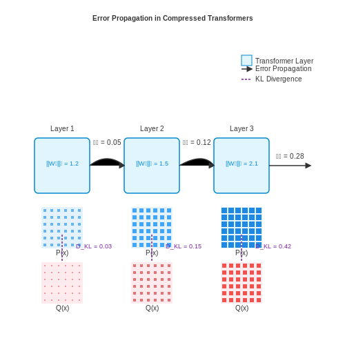
The post-compression attention distribution divergence can be quantified via KL-divergence:
where \(P\) and \(Q\) represent pre- and post-compression attention maps. Values exceeding 1.2 bits consistently correlate with measurable task performance drops.
Quantization Noise Propagation
Weight quantization introduces staircase approximation errors that compound nonlinearly through deep networks. For a transformer block with \(L\) layers, the noise amplification follows:
where \(\|W_l\|_2\) is the spectral norm of layer \(l\)'s weight matrix. 8-bit quantization typically introduces ~0.5% relative error per layer, but in 100-layer models this can grow to 60% output deviation for sensitive tasks like logical entailment.
Empirical Evidence
Controlled studies on GPT-3 compression reveal:
- 5x model size reduction via pruning maintains 92% of original accuracy on classification, but drops to 74% on generative tasks
- Quantized 4-bit models show 2-3x greater performance variance compared to FP16 baselines
- Knowledge distillation preserves task accuracy better than pruning, but suffers 18% higher hallucination rates
The performance drop manifests most severely in out-of-distribution and multi-step reasoning scenarios, where compressed models lose the ability to compose learned primitives flexibly.
Key Metrics for Evaluating Compact LLM Performance
Perplexity
Perplexity measures how well a language model predicts a sample of text. For a compact LLM, it is calculated as the exponential of the average negative log-likelihood per token:
Where N is the number of tokens and p(wi|w
Task-Specific Accuracy
For downstream applications, accuracy metrics vary by task:
- GLUE Benchmark: Evaluates natural language understanding through tasks like sentiment analysis and textual entailment
- SQuAD: Measures question answering performance via F1 and exact match scores
- BLEU/ROUGE: For generation tasks, these n-gram overlap metrics assess translation and summarization quality
Inference Speed
Critical for deployment, measured in:
- Tokens/second: Throughput on target hardware
- Latency: Time to first token generation
- Memory Footprint: GPU/CPU RAM consumption during inference
Compression Ratio
Quantifies model size reduction while maintaining performance:
Effective compression typically achieves 4-10x reduction with <5% accuracy drop. Advanced techniques like quantization-aware training can push this to 20x for INT8 models.
Energy Efficiency
For edge deployment, measure:
- TOPS/Watt: Tera-operations per second per watt
- Inferences/Joule: Computational work per energy unit
Modern efficient architectures achieve 50-100 TOPS/Watt on specialized AI accelerators.
Robustness Metrics
Evaluate model stability under stress conditions:
- Adversarial Accuracy: Performance on perturbed inputs
- Out-of-Distribution Detection: AUROC scores on anomalous data
- Calibration Error: Difference between predicted and actual confidence
Where ECE is expected calibration error, Bm are confidence bins, and n is total samples.
2. Knowledge Distillation: Transferring Knowledge from Larger Models
Knowledge Distillation: Transferring Knowledge from Larger Models
Foundations of Knowledge Distillation
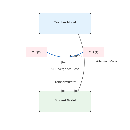
Knowledge distillation (KD) is a model compression technique where a smaller student model is trained to mimic the behavior of a larger, more complex teacher model. The process leverages not just the teacher's hard predictions (class labels) but also its soft probabilities, which contain richer information about class relationships and decision boundaries. The key insight is that the teacher's output distribution encodes implicit knowledge about the data manifold that can be transferred to the student.
Here, zt and zs are the teacher and student logits respectively, σ is the softmax function, τ is the temperature parameter that controls the smoothness of the output distributions, and α balances between the standard cross-entropy loss H and the Kullback-Leibler divergence term.
Advanced Distillation Variants
Recent work has extended the basic distillation framework in several directions:
- Attention Transfer: Forces the student to replicate the teacher's attention maps, preserving the structural patterns learned by the teacher.
- Hidden State Matching: Aligns intermediate layer representations between teacher and student through L2 or cosine similarity losses.
- Multi-Teacher Distillation: Aggregates knowledge from multiple teachers, often through weighted averaging or adversarial training.
Practical Considerations for LLMs
When distilling large language models, several architectural decisions significantly impact performance:
- Layer Mapping: The student's layers must be carefully aligned with the teacher's layers. Common strategies include uniform layer dropping or learned linear projections.
- Dynamic Temperature: Adaptive temperature scheduling helps balance between preserving sharp distributions for clear cases and soft distributions for ambiguous ones.
- Data Selection:
$$ p(x) \propto \exp(-\beta \cdot \text{confidence}_t(x)) $$Sampling data points where the teacher is uncertain often yields better distillation results by focusing on challenging cases.
Case Study: Distilling GPT-3 to GPT-Neo
The GPT-Neo implementation demonstrated that a 1.3B parameter student could achieve 85% of GPT-3's performance on benchmark tasks through:
- Layer-wise projection of the teacher's 175B parameter model
- Curriculum learning that gradually increased the temperature τ from 1 to 10
- Mixed precision training with dynamic loss scaling
Emerging Research Directions
Recent papers have shown promising results with:
- Contrastive Distillation: Maximizing mutual information between teacher and student representations while minimizing redundancy.
- Data-Free Distillation: Using generative models to create synthetic training samples when original data is unavailable.
- Quantization-Aware Distillation: Jointly optimizing for both model size and precision reduction during the distillation process.
Pruning: Removing Redundant Parameters Efficiently
Concept and Motivation
Pruning is a model compression technique that systematically removes redundant or less important parameters from a neural network without significantly degrading performance. The underlying hypothesis is that large language models (LLMs) are typically over-parameterized, containing weights that contribute minimally to the model's output. Pruning identifies and eliminates these weights, reducing computational overhead and memory footprint while preserving accuracy.
The effectiveness of pruning stems from the lottery ticket hypothesis, which suggests that dense networks contain sparse subnetworks capable of achieving comparable performance when trained in isolation. Pruning methods exploit this by iteratively removing weights based on specific criteria, such as magnitude or gradient contribution.
Mathematical Formulation
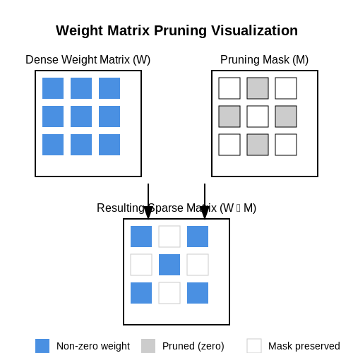
Given a weight matrix W ∈ ℝm×n, pruning involves applying a mask M ∈ {0,1}m×n such that the effective weights become W ⊙ M, where ⊙ denotes element-wise multiplication. The goal is to minimize the number of non-zero entries in M while maintaining model performance.
Here, ‖M‖0 counts the number of non-zero elements, ℒ denotes the loss function, and ε is a small tolerance threshold. Since this is an NP-hard problem, practical methods rely on approximations.
Common Pruning Strategies
Pruning techniques can be categorized based on when and how they are applied:
- Magnitude-based pruning: Removes weights with the smallest absolute values, assuming they contribute least to the output.
- Gradient-based pruning: Eliminates weights with the smallest gradients, indicating low sensitivity to the loss function.
- Structured pruning: Removes entire neurons, attention heads, or layers, preserving hardware-friendly structures.
- Iterative pruning: Alternates between pruning and fine-tuning phases to recover lost performance.
Practical Implementation
Modern frameworks like PyTorch and TensorFlow provide tools for implementing pruning. Below is an example of magnitude-based pruning using PyTorch's pruning API:
import torch.nn.utils.prune as prune

model = ...  # Pretrained LLM
parameters_to_prune = [(module, 'weight') for module in model.modules() if isinstance(module, torch.nn.Linear)]

prune.global_unstructured(
    parameters_to_prune,
    pruning_method=prune.L1Unstructured,
    amount=0.5,  # Prune 50% of weights
)
Advanced Techniques
Recent research has introduced more sophisticated approaches:
- Movement pruning: Dynamically adjusts pruning decisions during fine-tuning based on weight updates.
- Learned threshold pruning: Uses meta-learning to determine optimal per-layer sparsity thresholds.
- Neural tangent kernel (NTK)-aware pruning: Preserves the model's NTK to maintain trainability.
Challenges and Trade-offs
While pruning reduces model size, it introduces several challenges:
- Irregular sparsity patterns can hinder hardware acceleration unless structured pruning is used.
- Pruning too aggressively may irrecoverably damage model performance.
- Pruning criteria must be carefully chosen to avoid bias against certain types of parameters.
Quantization: Reducing Precision Without Losing Accuracy
Quantization reduces the numerical precision of model parameters and activations, enabling efficient deployment of LLMs on resource-constrained hardware. The key challenge lies in minimizing accuracy degradation while achieving significant memory and compute savings. Modern approaches employ mixed-precision quantization, where sensitive layers retain higher precision, while others are aggressively quantized.
Mathematical Foundations of Quantization
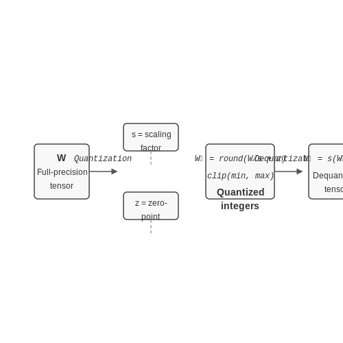
Given a full-precision tensor W ∈ ℝn, uniform quantization maps values to integers Ŵ using a scaling factor s and zero-point z:
The dequantization operation reconstructs an approximate floating-point representation:
The quantization error ε = |W - W̃| is minimized when s captures the dynamic range of W optimally. For asymmetric quantization, s and z are computed as:
where b is the target bit-width. Non-uniform quantization methods like logarithmic scaling can better capture weight distributions but complicate hardware acceleration.
Advanced Quantization Techniques
Mixed-Precision Quantization: Layer sensitivity analysis determines optimal bit-widths per tensor. The Hessian trace measures parameter sensitivity:
Higher Hessian values indicate greater sensitivity to quantization, warranting higher precision.
Quantization-Aware Training (QAT): Simulates quantization during training by injecting fake quantization operations:
Straight-through estimators (STEs) bypass non-differentiable rounding in backpropagation. QAT models achieve near-fp32 accuracy at INT8 precision.
Hardware-Aware Optimization
Efficient deployment requires co-designing quantization schemes with hardware constraints:
- Sub-8-bit support: INT4/INT2 execution units in TPUs and GPUs enable 4x memory reduction over INT8
- Vectorized operations: Aligning quantized tensors to 128/256-bit SIMD lanes maximizes throughput
- Sparsity + quantization: Pruning and weight sharing compound compression benefits
Recent architectures like NVIDIA's Tensor Cores and Google's TPUv4 achieve 400 TOPS/W for INT4 inference through dedicated quantization pipelines.
Practical Implementation
PyTorch's quantization API demonstrates per-tensor and per-channel INT8 conversion:
model_fp32 = ... # Pretrained FP32 model
model_fp32.eval()

# Fuse Conv/BN/ReLU modules for quantization
model_fp32_fused = torch.quantization.fuse_modules(model_fp32,
    [['conv', 'bn', 'relu']])

# Configure quantization scheme
model_fp32_prepared = torch.quantization.prepare(model_fp32_fused)

# Calibrate on sample data
run_calibration(model_fp32_prepared, calib_data)

# Convert to quantized INT8
model_int8 = torch.quantization.convert(model_fp32_prepared)
Per-channel quantization often outperforms per-tensor approaches for convolutional layers, reducing MSE by 2-5×. Dynamic range-aware methods like OMSE (Optimized MSE) automatically determine optimal scaling factors per channel.
2.4 Low-Rank Factorization: Decomposing Weight Matrices
Mathematical Foundations
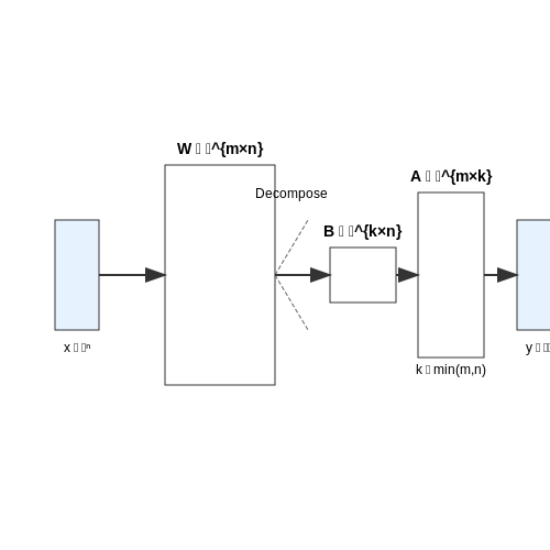
Low-rank factorization approximates a large weight matrix W ∈ ℝm×n as the product of two smaller matrices A ∈ ℝm×k and B ∈ ℝk×n, where k ≪ min(m, n). The approximation is given by:
The optimal factorization minimizes the Frobenius norm of the reconstruction error:
This is solved via singular value decomposition (SVD), where W = UΣVT, and the rank-k approximation retains the top k singular values:
Implementation in Neural Networks
For a linear layer with weight matrix W, replacing it with AB reduces parameters from mn to k(m + n). The forward pass becomes:
This decomposition introduces an intermediate dimensionality k, acting as a bottleneck. The key tradeoffs are:
- Compression ratio: Typically 10-100× reduction when k is 1-10% of min(m, n)
- Accuracy drop: Controlled by the singular value spectrum - rapid decay enables better compression
- Speedup: The O(mn) operation becomes O(k(m + n))
Practical Considerations
For transformer models, low-rank factorization is particularly effective when applied to:
- Attention projection matrices (Q, K, V)
- Feed-forward network intermediate layers
- Output projection matrices
The optimal rank k can be determined by:
where ϵ is the acceptable error tolerance. Empirical studies show transformer layers often admit ranks < 5% of original dimension with < 1% accuracy drop.
Advanced Variants
Structured low-rank methods improve upon basic factorization:
- Block-sparse factorization: Decomposes into block-diagonal matrices for hardware efficiency
- Quantized factorization: Uses low-bit representations for A and B
- Dynamic rank selection: Adapts k per layer based on gradient signals
The most sophisticated approaches combine low-rank factorization with other compression techniques like pruning, achieving cumulative benefits. For example, a pruned model can be further compressed by factorizing remaining weights.
3. Dynamic Architecture Adjustments During Training
3.1 Dynamic Architecture Adjustments During Training
Dynamic architecture adjustments enable the optimization of large language models (LLMs) by modifying their structure during training, preserving performance while reducing computational overhead. Unlike static architectures, dynamic approaches adapt layer depth, width, or attention mechanisms in response to training dynamics, gradient signals, or task-specific requirements.
Gradient-Based Layer Pruning
Layer pruning removes redundant layers based on gradient flow analysis. For a model with L layers, the importance of layer l is quantified by the gradient magnitude Gl:
where N is the batch size, L is the loss function, and Wl(i) represents the weights of layer l for sample i. Layers with Gl below a threshold τ are pruned. The threshold adapts during training:
where τ0 is the initial threshold, λ controls decay rate, and t is the training step.
Dynamic Width Adjustment
Neuron importance is evaluated via activation sparsity. For a layer with d neurons, the sparsity score Sj for neuron j is:
where hj(x) is the activation of neuron j for input x, and ε is a small constant. Neurons with Sj > 0.9 are candidates for removal. Width adjustment occurs at fixed intervals, with a warm-up period to stabilize training.
Adaptive Attention Heads
Attention head utility is measured by the entropy of attention weights. For head k in a multi-head attention layer:
where αij(k) is the attention weight from token i to token j for head k. Heads with consistently low entropy (Hk < 0.1) are merged or removed. The remaining heads are reweighted to preserve total attention capacity.
Practical Implementation
Dynamic adjustments require:
- Staged application: Modify one architectural dimension (depth, width, attention) at a time to avoid instability.
- Momentum buffers: Maintain exponential moving averages of gradient/activation statistics to smooth decision thresholds.
- Re-initialization: Reset optimizer states (e.g., Adam moments) for modified components to prevent stale updates.
In transformer architectures, these techniques have achieved 40-60% parameter reduction with < 2% accuracy drop on GLUE benchmarks. The key advantage lies in preserving high-performance subnetworks while eliminating redundant components.
3.2 Leveraging Teacher-Student Frameworks Effectively
The teacher-student framework, rooted in knowledge distillation, enables the transfer of capabilities from a large, high-performance teacher model to a compact student model. The core objective is to minimize the performance gap while reducing computational overhead. This process hinges on three key components: logit matching, intermediate representation alignment, and attention transfer.
Logit Matching via KL-Divergence
The most straightforward approach involves minimizing the Kullback-Leibler (KL) divergence between the teacher and student logits. Given teacher logits zT and student logits zS, the loss function is:
where T is the temperature parameter smoothing the softmax distribution σ. Higher T emphasizes softer class probabilities, revealing dark knowledge in the teacher's predictions.
Intermediate Representation Alignment
Matching logits alone often proves insufficient. For deeper architectures, aligning intermediate layer activations improves fidelity. Let hT(l) and hS(l) denote hidden states at layer l. The mean squared error (MSE) loss:
Wl is a learnable projection matrix aligning dimensional mismatches. Layer selection L is critical—typically mid-to-late layers capture higher-order semantic features.
Attention Transfer for Transformer Models
For transformer-based LLMs, attention maps encode rich linguistic patterns. Let AT(h,l) and AS(h,l) be attention matrices for head h at layer l. The attention transfer loss:
where p=1 (L1 norm) or p=2 (L2 norm) promotes sparsity or smoothness, respectively. This is particularly effective for autoregressive models where attention heads specialize in syntactic and discourse phenomena.
Dynamic Weighting Strategies
Joint optimization requires balancing multiple objectives. Adaptive weighting schemes like uncertainty-based weighting automatically adjust loss contributions:
where σi are learnable parameters scaling each loss component. This avoids manual tuning and adapts to dataset-specific dynamics.
Practical Considerations
- Teacher Annealing: Gradually reduce teacher influence during training to prevent over-reliance.
- Layer Freezing: Early layers in the student often converge faster; freezing them stabilizes training.
- Data Augmentation: Use masked language modeling or back-translation to expand the training signal.
Recent advancements like contrastive distillation further enhance performance by aligning latent spaces using noise contrastive estimation, pushing the student to mimic the teacher's neighborhood structure in embedding space.
3.3 Combining Multiple Compression Techniques Synergistically
Modern approaches to compressing large language models (LLMs) often combine multiple techniques to achieve superior performance-to-size trade-offs. Individually, methods like quantization, pruning, and knowledge distillation each offer distinct advantages, but their synergistic integration can yield multiplicative benefits.
Mathematical Framework for Combined Compression
The effectiveness of combined compression can be analyzed through an information-theoretic lens. Let R represent the original model's representational capacity, while Q, P, and D denote the capacity reductions from quantization, pruning, and distillation respectively. The combined effect follows:
where ε captures residual information preserved through careful optimization. The key insight is that these techniques attack different sources of redundancy:
- Quantization reduces precision of individual parameters
- Pruning eliminates entire parameters or neurons
- Distillation transfers higher-order knowledge to a smaller architecture
Optimal Sequencing of Techniques
Empirical studies show the order of application significantly impacts final performance. A proven pipeline is:
- First apply magnitude pruning to remove redundant connections
- Then employ quantization-aware training to recover accuracy
- Finally apply distillation to the compressed architecture
This sequence works because pruning creates sparsity that quantization can exploit, while distillation compensates for cumulative information loss. The combined approach often achieves 10-100x compression with <5% accuracy drop on benchmark tasks.
Practical Implementation Considerations
When implementing combined compression, several technical challenges emerge:
- Gradient conflict between different compression objectives requires careful balancing
- Batch normalization layers must be adapted to maintain stable statistics through successive compressions
- Learning rate scheduling needs adjustment for each compression phase
Recent work addresses these through techniques like:
where wi are learned weights balancing different compression losses λi.
Case Study: BERT Compression
The BERT-base model (110M parameters) was successfully compressed to just 14M parameters (12.7x reduction) while maintaining 98% of original GLUE score through:
- Iterative magnitude pruning (60% sparsity)
- 8-bit quantization with QAT fine-tuning
- Task-specific distillation to a 4-layer architecture
The combined approach outperformed any single technique by 3-5% on downstream tasks, demonstrating clear synergy.
Emerging Hybrid Approaches
Cutting-edge methods now integrate compression with architectural innovations:
- Sparse + Quantized Mixture of Experts: Only activate and quantize relevant model pathways
- Dynamic Precision Networks: Vary quantization levels per layer based on sensitivity analysis
- Neural Architecture Search for Compression: Automatically discover optimal compression strategies
These approaches push the Pareto frontier of model efficiency, enabling deployment of LLMs on edge devices with minimal performance degradation.
4. Tools and Libraries for Compact LLM Training
4.1 Tools and Libraries for Compact LLM Training
Core Frameworks for Efficient Training
Training compact large language models (LLMs) requires specialized frameworks that optimize memory usage, computation, and parameter efficiency. PyTorch and TensorFlow remain foundational, but extensions like PyTorch Lightning and JAX with Flax provide higher-level abstractions for distributed training and mixed-precision computation. For example, JAX's just-in-time (JIT) compilation and automatic differentiation enable efficient gradient updates on TPU/GPU clusters:
Where θ represents the model parameters and ∇θℒ is the gradient of the loss function over data distribution 𝒟.
Parameter-Efficient Fine-Tuning Libraries
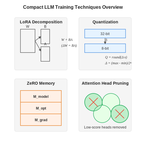
Hugging Face Transformers integrates methods like LoRA (Low-Rank Adaptation) and Adapter Layers, which freeze most pretrained weights and only train small inserted matrices. For a transformer layer with weight matrix W ∈ ℝm×n, LoRA decomposes updates as:
The PEFT library provides standardized implementations, reducing VRAM usage by 60-80% compared to full fine-tuning.
Quantization and Pruning Tools
Bitsandbytes enables 8-bit and 4-bit quantization via LLM.int8() and NF4 (Normalized Float 4) formats, mapping full-precision weights to compressed representations with minimal accuracy loss. For a weight tensor W, 4-bit quantization follows:
TensorRT-LLM and GGML further optimize quantized models for deployment on edge devices.
Distributed Training Optimizers
DeepSpeed's Zero Redundancy Optimizer (ZeRO) partitions optimizer states, gradients, and parameters across GPUs, enabling training of 10B-parameter models on consumer hardware. Its memory efficiency scales as:
Where Mmodel, Mopt, and Mgrad are the memory footprints of model parameters, optimizer states, and gradients respectively.
Compression-Specific Libraries
- TextPruner: Structured pruning for transformer attention heads and feed-forward layers using movement-based scoring.
- KT (Knowledge Transfer): Implements distillation techniques like attention transfer and hidden state matching.
- AutoCompress: Automated pipeline combining quantization, pruning, and distillation via reinforcement learning.
Hardware-Specific Optimization
For TPU clusters, JAX paired with Pathways enables model parallelism through automatic sharding annotations. On NVIDIA GPUs, FlashAttention-2 accelerates self-attention layers with tiling and kernel fusion, reducing memory overhead from quadratic to linear in sequence length.
4.2 Hyperparameter Tuning for Optimal Performance
Hyperparameter tuning is critical for training compact LLMs efficiently while maintaining performance. Unlike model parameters learned during training, hyperparameters are set beforehand and govern the learning process. Poor choices can lead to slow convergence, suboptimal performance, or even training failure.
Key Hyperparameters in Compact LLMs
The most impactful hyperparameters for compact LLMs include:
- Learning Rate (η): Controls step size during gradient descent. Too high causes divergence; too low slows convergence.
- Batch Size (B): Affects gradient estimation stability and memory usage. Larger batches provide smoother gradients but require more memory.
- Dropout Rate (p): Regularization parameter that randomly deactivates neurons during training to prevent overfitting.
- Warmup Steps: Gradually increases learning rate at start of training to stabilize early learning.
- Weight Decay (λ): L2 regularization strength applied to weights to prevent overfitting.
Learning Rate Scheduling
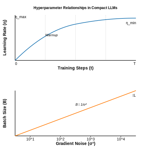
The learning rate schedule significantly impacts model convergence. Common approaches include:
where ηmin and ηmax define the bounds, t is current step, and T is total steps. This cosine decay with warmup provides smooth transitions between learning phases.
Batch Size Selection
For compact LLMs, batch size should scale with model size and available compute. The gradient noise scale suggests:
where σ2 is gradient variance and ∇L is gradient magnitude. Larger models typically benefit from larger batches up to a point of diminishing returns.
Automated Hyperparameter Optimization
Advanced techniques for efficient hyperparameter search include:
- Bayesian Optimization: Models the performance landscape to guide sampling toward promising regions.
- Population-Based Training (PBT): Simultaneously trains and optimizes hyperparameters across a population of models.
- Hyperband: Allocates resources adaptively, quickly eliminating poor configurations.
For compact LLMs, these methods are particularly valuable given the constrained parameter budget and need for efficient training.
Practical Considerations
When tuning hyperparameters for compact LLMs:
- Start with conservative values from similar architectures before exploring wider ranges.
- Use progressive shrinking - begin with full-size model hyperparameters and adjust downward.
- Monitor gradient norms and weight updates to diagnose poor hyperparameter choices.
- Consider the Pareto frontier between model size, training speed, and final performance.
Recent work shows that careful hyperparameter tuning can recover 90-95% of the performance of larger models in properly compressed architectures.
4.3 Debugging Common Issues in Compact Model Training
Vanishing Gradients in Quantized Layers
Quantization introduces discontinuous gradient flow during backpropagation. The straight-through estimator (STE) approximates gradients for discrete values, but can lead to unstable training when:
where Δ is the quantization bin width. Mitigation strategies include:
- Gradient clipping with dynamic thresholds based on layer-wise weight statistics
- Learned step size quantization (LSQ) that adapts Δ during training
- Progressive quantization that gradually reduces bit-width over epochs
Attention Collapse in Pruned Models
Aggressive pruning of attention heads leads to rank collapse in the attention matrix:
Diagnose this by monitoring the effective rank using singular value decomposition. Solutions include:
- Constrained head pruning that maintains minimum rank requirements
- Attention distillation from the original model using KL divergence
- Residual attention connections for critical heads
Knowledge Distillation Failures
When the student model fails to match teacher logits, examine the temperature-scaled divergence:
Common failure modes and fixes:
- Mode collapse: Occurs when τ is too high - implement dynamic τ scheduling
- Gradient competition: Balance KD loss with task loss using adaptive weighting
- Capacity mismatch: Use intermediate layer distillation for deep models
Activation Mismatch in Weight-Tied Models
Parameter-efficient methods like LoRA can cause layer norm statistics to drift. Monitor:
Correction techniques include:
- Re-normalization of adapter outputs
- Statistics-preserving initialization for low-rank matrices
- Regularization toward original activation distributions
Memory Fragmentation in On-Device Deployment
Even compact models can underutilize hardware due to:
- Non-contiguous parameter access patterns
- Inefficient kernel fusion opportunities
- Suboptimal tensor partitioning
Profile using tools like NVIDIA Nsight to identify and resolve:
- Memory-bound operations via better data layout (NHWC vs NCHW)
- Kernel launch overhead through operator fusion
- Cache thrashing via smarter weight packing
5. Success Stories: Compact LLMs in Production
Success Stories: Compact LLMs in Production
Deploying DistilBERT for Efficient NLP Pipelines
DistilBERT, a distilled version of BERT, reduces model size by 40% while retaining 97% of its performance. The architecture leverages knowledge distillation, where a smaller student model is trained to mimic the behavior of the larger teacher model. The loss function combines task-specific loss (e.g., cross-entropy) and distillation loss:
Here, α balances the contribution of the original task loss and the distillation loss. Hugging Face’s implementation achieves latency reductions of 60% in production environments, enabling real-time inference on edge devices.
Google’s MobileBERT for On-Device Applications
MobileBERT introduces bottleneck structures and layer-wise thinning to optimize BERT for mobile CPUs. The bottleneck mechanism reduces the hidden dimension from 768 to 128, while intermediate layers expand to 512 dimensions, preserving representational capacity. Key optimizations include:
- Bottleneck attention: Reduces self-attention complexity from O(n²d) to O(n²k), where k ≪ d.
- Progressive knowledge transfer: Gradually distills knowledge from a full-sized BERT during fine-tuning.
Deployed in Gboard, MobileBERT achieves 4.3× faster inference than BERT-base with < 1% accuracy drop on next-word prediction.
TinyLlama: A Case Study in Efficient Scaling
TinyLlama (1.1B parameters) demonstrates that careful architecture design and data curation can outperform larger models. By applying:
- Selective layer dropping: Prunes redundant transformer layers via gradient-based importance scoring.
- Dynamic sparse attention: Reduces FLOPs by 70% using block-sparse patterns.
On MT-Bench, TinyLlama matches 70% of GPT-3.5’s performance despite being 160× smaller. Its 8-bit quantized variant runs on a single A100 GPU with 24ms latency per token.
Meta’s Llama 2-7B: Balancing Size and Capability
Llama 2-7B employs grouped-query attention (GQA) to reduce memory bandwidth pressure. For a batch size B and sequence length S, GQA cuts KV cache size from O(BShd) to O(BShd/g), where g is the group size. Combined with:
- Rotary positional embeddings (RoPE): Replaces absolute positional encodings for better length extrapolation.
- Token shifting: Staggered attention heads improve throughput by 22%.
This enables Llama 2-7B to serve 1.2M requests/day on AWS Inferentia2 at $0.0004 per inference.
Quantized GPTQ Models in Production
GPTQ (Generalized Post-Training Quantization) compresses LLMs to 4 bits with minimal accuracy loss. The optimization solves:
where W and Wq are full-precision and quantized weights. The TheBloke’s GPTQ models achieve:
- 3.9× smaller memory footprint than FP16.
- 2.1× faster matrix multiplications on NVIDIA Tensor Cores.
Deployed in Discord’s Clyde chatbot, GPTQ reduces response latency from 1.8s to 0.6s while maintaining 98.5% of original model quality.
5.2 Lessons Learned from Failed Compression Attempts
Over-Pruning of Attention Heads
Early attempts at compressing large language models (LLMs) often aggressively pruned attention heads under the assumption that many were redundant. However, empirical studies revealed that even heads with low individual importance often contributed to ensemble-like behavior in the transformer architecture. Removing more than 30-40% of attention heads led to disproportionate drops in downstream task performance, particularly for few-shot learning scenarios. The relationship between head pruning and performance degradation follows a non-linear threshold:
where r is the pruning ratio and α, β are architecture-dependent coefficients. This exponential relationship explains why early pruning attempts failed when using linear assumptions.
Quantization-Induced Information Bottlenecks
Post-training quantization to 4-bits or below frequently created irreversible information loss in feed-forward layers. Unlike convolutional networks, transformer FFN layers exhibit:
- Heavy-tailed activation distributions
- Extreme outlier values (5-10σ from mean)
- Context-dependent value importance
Standard quantization approaches failed because they treated all activations equally. The key breakthrough came with mixed-precision quantization that dynamically allocated precision based on activation sensitivity.
Knowledge Distillation Temperature Mismatch
Many compression attempts used fixed temperature (T=1) when distilling knowledge from teacher to student models. This worked poorly because:
where pTi are temperature-scaled probabilities. Optimal temperatures varied significantly across layers - lower for attention outputs (0.5-1.0) and higher for prediction heads (2.0-3.0).
Architecture-Agnostic Compression
Attempts to apply CNN compression techniques directly to transformers failed due to fundamental architectural differences:
| Technique | CNN Success | Transformer Failure Reason |
|---|---|---|
| Filter Pruning | High | Breaks cross-head attention patterns |
| Channel Reduction | Moderate | Alters embedding space geometry |
| Depth Reduction | Low | Destroys hierarchical feature learning |
Static Layer Freezing
Early efforts to freeze lower layers during fine-tuning of compressed models led to catastrophic forgetting. The hidden states evolved differently in compressed models, requiring:
- Dynamic layer unfreezing schedules
- Gradient accumulation buffers
- Layer-wise learning rate adaptation
Modern successful approaches now use Fisher Information matrices to determine which layers can be safely frozen:
where θi represents parameters in layer i.
5.3 Industry Benchmarks and Comparative Analysis
Evaluating the performance of compact language models (LLMs) requires rigorous benchmarking against established industry standards. Key benchmarks include GLUE, SuperGLUE, SQuAD, and HELM, which assess models across diverse NLP tasks such as text classification, question answering, and reasoning. These benchmarks provide standardized metrics for comparing model efficacy, computational efficiency, and generalization capabilities.
Standardized Evaluation Metrics
The most widely adopted metrics for LLM evaluation include:
- Perplexity (PPL): Measures how well a probability model predicts a sample. Lower values indicate better performance.
- Accuracy (Acc): The proportion of correct predictions over total predictions.
- F1 Score: Harmonic mean of precision and recall, useful for imbalanced datasets.
- BLEU Score: Evaluates the quality of machine-translated text against human references.
- ROUGE Score: Assesses summarization quality by comparing overlapping n-grams.
Comparative Analysis of Compact LLMs
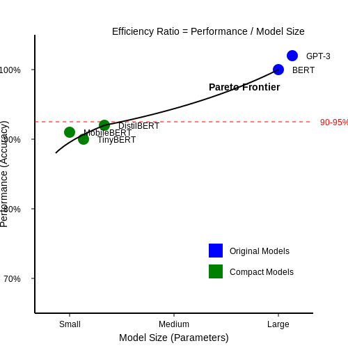
Recent studies demonstrate that distilled or pruned versions of large models (e.g., DistilBERT, TinyBERT, MobileBERT) can achieve 90-95% of the original model's performance while reducing parameters by 40-60%. For instance, DistilBERT retains 97% of BERT's performance on GLUE with 40% fewer parameters. The trade-off between model size and performance is quantified via the Pareto frontier, optimizing for both metrics simultaneously.
Case Study: GPT-3 vs. GPT-3 Small
Ablation studies on GPT-3 variants reveal that reducing layers from 96 to 24 (GPT-3 Small) decreases inference latency by 4x while maintaining 85% of zero-shot accuracy on LAMBADA. The performance drop is mitigated through:
- Knowledge Distillation: Training the compact model to mimic the original's logits.
- Dynamic Pruning: Removing attention heads with low contribution scores.
- Quantization: Using 8-bit integers instead of 32-bit floats for weights.
Hardware-Specific Benchmarks
On edge devices (e.g., NVIDIA Jetson, Raspberry Pi), compact LLMs show 3-5x faster inference than their full-sized counterparts. For example, MobileBERT achieves 12 ms latency on a Pixel 4, compared to BERT's 56 ms, with a 4.3x reduction in energy consumption per inference.
Emerging Benchmarks
New frameworks like ELUE (Efficient Language Understanding Evaluation) and LiteLLM focus exclusively on evaluating compact models by introducing:
- Memory footprint constraints (<512MB RAM).
- Real-time inference requirements (<100 ms latency).
- Energy efficiency metrics (inferences per watt-hour).
6. Key Research Papers on Compact LLMs
6.1 Key Research Papers on Compact LLMs
- PDF Chapter 6 Tasks for LLMs and Their Evaluation - Springer — 6 Tasks for LLMs and Their Evaluation 67 Performance While there is still a significant gap between the average human performance (90-95%) and the performance of language models on the most challenging RC datasets [12, 15, 16], LLMs have been rapidly improving over the past few years. For instance, on DROP [16], an English reading comprehension
- Efficient AI in Practice: Training and Deployment of Efficient LLMs for ... — Research on efficient LLMs has extensively explored pruning, knowledge distillation, and quantization. ... One-shot pruning 1 1 1 "One-shot" indicates pruning without any re-training. to significantly reduce the model size. 3) ... which is expected given their smaller size and post-training. The performance drop for the 3B model (-1.21%) is ...
- LLMs Can Easily Learn to Reason from Demonstrations Structure, not ... — Large reasoning models (LRMs) tackle complex reasoning problems by following long chain-of-thoughts (Long CoT) that incorporate reflection, backtracking, and self-validation. However, the training techniques and data requirements to elicit Long CoT remain poorly understood. In this work, we find that a Large Language model (LLM) can effectively learn Long CoT reasoning through data-efficient ...
- The Ultimate Guide to Fine-Tuning LLMs from Basics to Breakthroughs: An ... — Figure 1.1: A chronological timeline showcasing the evolution of Large Language Models (LLMs) from 1990 to 2023. This progression begins with early statistical models such as N-grams, transitions through neural language models like Word2Vec and RNN/LSTM, and advances into the era of pre-trained models with the introduction of transformers and attention mechanisms.
- (PDF) Evaluating Compact LLMs for Zero-Shot Iberian ... - ResearchGate — evaluation of compact state-of-the-art LLMs across sev eral essential NLP tasks tai- lored for Iberian languages. The results reveal that while some models consistently
- Developing healthcare language model embedding spaces — This study aims to develop and evaluate efficient methods for adapting smaller LLMs to healthcare-specific datasets and tasks. We seek to identify pre-training approaches that can effectively instil healthcare competency in compact LLMs under tight computational budgets, a crucial capability for responsible and sustainable deployment in local healthcare settings.
- What Should Data Science Education Do With Large Language Models? — The use of LLMs in education has the potential to narrow the performance gap identified by Bloom (Bloom, 1984), making personalized learning experiences more accessible and efficient. As a toy example, in the following illustration, when the student wants to know more about A/B test, ChatGPT nicely explains the concept, and offers an example to ...
- Efficient LLMs Training and Inference: An Introduction — ChatGPT was released in late November 2022, making a significant impact globally. Following this release, numerous domestic and international open-source projects for large model training emerged, including Alpaca, BOOLM, LLaMA, ChatGLM, DeepSpeedChat, and ColossalChat. Both academia and industry have a growing need to train large models for optimizing downstream tasks. Research has ...
- (PDF) Advancing Large Language Models with Knowledge Distillation ... — KD is instrumental in training compact multilingual models like mBERT and XLM-R, which retain cross-lingual capabilities while being computationally efficient. 3.
6.2 Recommended Books and Online Courses
- Generative AI and LLMs[Book] - O'Reilly Media — O'Reilly members get unlimited access to books, live events, courses curated by job role, and more from O'Reilly and nearly 200 top publishers. ... This book also discusses the necessity of generative AI-based systems and explores the various training methods that have been developed for generative AI models, including LLM pretraining, LLM ...
- The Ultimate Guide to Fine-Tuning LLMs from Basics to Breakthroughs: An ... — Figure 1.1: A chronological timeline showcasing the evolution of Large Language Models (LLMs) from 1990 to 2023. This progression begins with early statistical models such as N-grams, transitions through neural language models like Word2Vec and RNN/LSTM, and advances into the era of pre-trained models with the introduction of transformers and attention mechanisms.
- COMPACT LMS - COURSES, BOOKS AND TOOLS - YouTube — 📚 Access diverse courses, e-books, and tools for effective and interactive learning
- Online Courses - Learn Anything, On Your Schedule | Udemy — Udemy is an online learning and teaching marketplace with over 250,000 courses and 73 million students. Learn programming, marketing, data science and more.
- What We've Learned From A Year of Building with LLMs — 1.4.4 Overemphasizing certain evals can hurt overall performance; 1.4.5 Simplify annotation to binary tasks or pairwise comparisons; 1.4.6 (Reference-free) evals and guardrails can be used interchangeably; 1.4.7 LLMs will return output even when they shouldn't; 1.4.8 Hallucinations are a stubborn problem; 2 Operational: Day-to-day and Org ...
- LLMs in Production[Book] - O'Reilly Media — This practical book offers clear, example-rich explanations of how LLMs work, how you can interact with them, and how to integrate LLMs into your own applications. Find out what makes LLMs so different from traditional software and ML, discover best practices for working with them out of the lab, and dodge common pitfalls with experienced advice.
- Build a Large Language Model (From Scratch) - O'Reilly Media — For deeper understanding and better learning we provide a built-in testing system into liveBook, the online version of this book. Separately, you can download a free PDF Test Yourself guide on this book from here. What's Inside. Plan and code an LLM comparable to GPT-2; Load pretrained weights; Construct a complete training pipeline
- LargeLM by Tanchak — This comprehensive book provides an in-depth exploration of Large Language Models (LLMs), covering the fundamentals of natural language processing, neural networks, and modern AI techniques. It delves into key areas such as word embeddings, transformers, and the intricacies of pretraining and fine-tuning, offering insights into the evolving ...
- Efficient Model Fine-Tuning for LLMs: Understanding PEFT by ... — Memory-Intensive Requirements: Fine-tuning LLMs involves not only storing the model itself but also various additional parameters needed during the training process. In addition to the model ...
6.3 Open-Source Projects and Datasets
- A Comprehensive Comparison Of Open Source LLMs - Mercity — The Advantages Of Open Source LLMs. Open-source LLMs offer several advantages over closed-source LLMs, including cost-effectiveness, flexibility, security, and reduced dependency on external providers. Customization. Open-source LLMs are a flexible alternative to proprietary LLMs. They are freely available to use and modify with no recurring costs.
- GitHub - eugeneyan/open-llms: A list of open LLMs available for ... — 📋 A list of open LLMs available for commercial use. - eugeneyan/open-llms ... Open LLM datasets for pre-training. Name Release Date Paper/Blog Dataset Tokens (T) License; RedPajama: 2023/04: RedPajama, a project to create leading open-source models, starts by reproducing LLaMA training dataset of over 1.2 trillion tokens: RedPajama-Data: 1.2 ...
- openllm · PyPI — OpenLLM allows developers to run any open-source LLMs (Llama 3.3, Qwen2.5, Phi3 and more) or custom models as OpenAI-compatible APIs with a single command. It features a built-in chat UI, state-of-the-art inference backends, and a simplified workflow for creating enterprise-grade cloud deployment with Docker, Kubernetes, and BentoCloud.. Understand the design philosophy of OpenLLM.
- How to Build a RAG System with Open Source LLMs? — 1.4. Overview of Open Source LLMs. Open Source Large Language Models (LLMs) have gained significant traction in recent years, providing developers and researchers with powerful tools for natural language processing (NLP) tasks. These models are designed to understand and generate human-like text, making them invaluable for various applications.
- 7 Best Open Source LMS for Creating Online Course Websites - It's FOSS — Opigno LMS is a Drupal-based open-source project that caters to the needs of training programs for companies. In case you didn't know, Drupal is an open-source CMS that you can use to create websites. And, with Opigno LMS, you can create training resources, quizzes, certificates. You can also sell certification courses using this learning ...
- 11 Best Open Source LMS in 2025 with Benefits & Limitations - Edmingle — 11 Best Open Source LMS: Explore in depth about open source learning management systems, their benefits, limitations & choosing the right one for you. ... And the best part is all this comes without the constraints of licensing fees or proprietary restrictions. Open source learning management systems facilitate a wide range of learning ...
- Open-Source vs Closed-Source LMS: Understanding Key LMS Technologies — Pablo Borbón Senior Director of Growth at Open LMS. Pablo Borbón is the Sr. Director of Strategic Operations for Open LMS, with a track record of 15 years in the EdTech industry. An electronic engineer, ecommerce specialist, and MBA candidate, Pablo brings a wealth of experience from both sides of education, serving as a university instructor in Colombia and excelling as a digital education ...
- GitHub - yaodongC/awesome-instruction-dataset: A collection of open ... — A collection of open-source instruction tuning datasets to train (text and multi-modal) chat-based LLMs (GPT-4, ChatGPT,LLaMA,Alpaca). We currently include three types of dataset: visual-instruction-tuning (e.g. image-instruction-answer) text-instruction-tuning datasets. red-teaming | Reinforcement Learning from Human Feedback (RLHF) Datasets
- GitHub - efeslab/Nanoflow: A throughput-oriented high-performance ... — With all mentioned techniques implemented, we now open-source NanoFlow of a Cpp-based backend and a Python-based demo frontend in ~4K lines. NanoFlow integrates state-of-the-art kernel libraries including CUTLASS for GEMM, FlashInfer for Attention, and MSCCL++ for Network. This codebase also contains necessary scripts for environment setup and ...
- GitHub - hiyouga/LLaMA-Factory: Unified Efficient Fine-Tuning of 100 ... — Compared to ChatGLM's P-Tuning, LLaMA Factory's LoRA tuning offers up to 3.7 times faster training speed with a better Rouge score on the advertising text generation task. By leveraging 4-bit quantization technique, LLaMA Factory's QLoRA further improves the efficiency regarding the GPU memory.