Building a Customer Service Chatbot with RAG
1. What is Retrieval-Augmented Generation (RAG)?
What is Retrieval-Augmented Generation (RAG)?
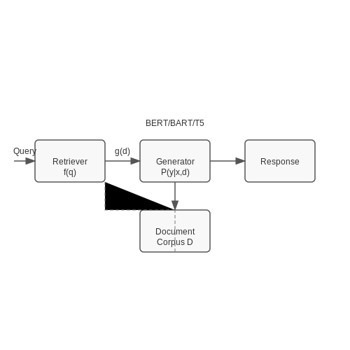
Retrieval-Augmented Generation (RAG) is a hybrid architecture that combines the strengths of dense retrieval and generative language models to produce contextually grounded responses. Unlike traditional language models that rely solely on parametric memory, RAG dynamically retrieves relevant documents from an external knowledge source and conditions its generation on this retrieved context. This approach addresses key limitations of pure autoregressive models, such as hallucination and outdated knowledge, by grounding responses in verifiable external data.
Architectural Components
The RAG framework consists of two primary components:
- Retriever: A dense passage retrieval (DPR) model that encodes both queries and documents into a shared embedding space. Given a query q, it returns the top-k most relevant documents D from a corpus C based on maximum inner product search (MIPS):
where f and g are query and document encoders respectively, typically implemented as BERT-style transformers.
- Generator: A seq2seq model (e.g., BART or T5) that produces the final output by attending to both the input query and retrieved documents. The generation probability is factorized as:
Training Paradigm
RAG is trained end-to-end using a marginal likelihood objective that jointly optimizes both components:
The retriever is trained using gradient backpropagation through the non-differentiable retrieval step via the REINFORCE algorithm, with the generator's sequence likelihood serving as the reward signal.
Advantages Over Pure LM Approaches
- Knowledge Freshness: By retrieving from updatable document stores, RAG avoids the static knowledge limitation of frozen LM parameters
- Verifiability: Source documents provide provenance for generated claims, enabling fact-checking
- Scalability: Knowledge capacity grows with the document corpus size rather than model parameters
- Computational Efficiency: Avoids the quadratic memory overhead of storing all knowledge in model weights
Practical Implementation Considerations
Effective RAG systems require careful engineering of several components:
- Document Chunking: Optimal segmentation of source material into retrievable units (typically 100-300 words)
- Embedding Index: Efficient approximate nearest neighbor search using FAISS or similar libraries
- Fusion Strategies: Techniques like reciprocal rank fusion for combining multiple retrieved passages
- Generation Conditioning: Architectural variants like FiD (Fusion-in-Decoder) that process documents independently
Recent advances like RAG-Token (per-token retrieval) and RAG-Sequence (per-output retrieval) provide additional flexibility in how retrieved knowledge is incorporated into the generation process. The choice between these variants depends on the specific use case's requirements for consistency versus diversity in responses.
Why Use RAG for Customer Service Chatbots?
Retrieval-Augmented Generation (RAG) architectures address critical limitations of traditional generative models in customer service applications by dynamically grounding responses in external knowledge. Unlike purely parametric models, which rely solely on pre-trained weights and often hallucinate facts, RAG combines the strengths of dense retrieval and neural generation.
Knowledge Freshness and Dynamic Updates
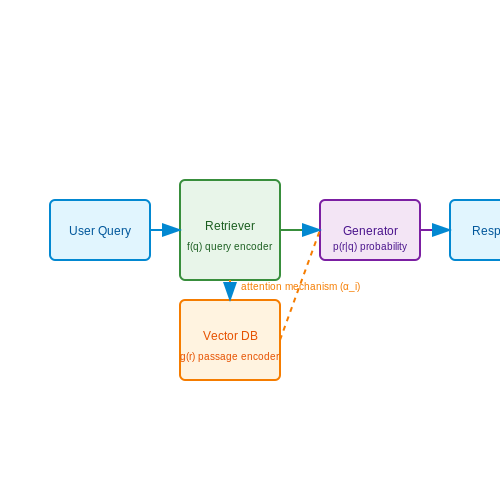
Customer service domains require up-to-date information, such as policy changes, product updates, or troubleshooting guides. Traditional fine-tuned models suffer from knowledge cutoff issues, requiring expensive retraining. RAG circumvents this by retrieving from a vector database that can be updated in real-time. The retrieval probability p(r|q) for a query q is computed as:
where f and g are query and passage encoders, and R is the retrieval corpus. This allows seamless integration of new documentation without model retraining.
Verifiability and Audit Trails
RAG provides explicit provenance by attaching source documents to generated responses. This is critical for compliance-sensitive industries like healthcare or finance. The attention mechanism in the generator highlights which retrieved passages contributed to the output:
where hret are retrieved passage embeddings and W is a learned projection matrix.
Cost-Efficiency in Production
RAG architectures demonstrate superior cost-performance tradeoffs compared to monolithic LLMs. By offloading factual recall to the retrieval system, the generator can be a smaller, more efficient model. The end-to-end latency L decomposes as:
where n is response length. This sublinear scaling enables handling large knowledge bases with minimal GPU resources.
Multimodal Customer Support
Advanced RAG implementations extend beyond text to handle tickets containing screenshots, error logs, or product diagrams. Cross-modal encoders like CLIP enable joint embedding spaces:
where s(I,T) measures image-text similarity. This allows the chatbot to reference visual materials during troubleshooting.
Domain Adaptation Strategies
RAG systems outperform fine-tuned models in low-data regimes by leveraging pretrained components. The dual-encoder architecture permits independent optimization:
- Retriever: Fine-tuned via contrastive learning on domain-specific query-passage pairs
- Generator: Initialized from general-purpose LLMs with lightweight adapter layers
This modularity reduces the need for large annotated datasets while maintaining performance.
1.3 Key Components of a RAG System
Retriever Module
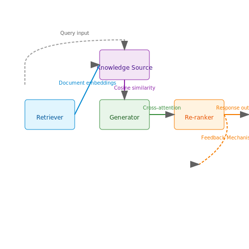
The retriever is responsible for fetching relevant documents from a knowledge source given an input query. Modern RAG systems typically employ dense retrieval methods, where both the query and documents are embedded into a shared vector space using a transformer-based encoder such as BERT or RoBERTa. The similarity between query and document embeddings is computed using cosine similarity:
where q and d are the query and document embeddings respectively. The top-k documents with highest similarity scores are retrieved for subsequent processing. Advanced systems may use approximate nearest neighbor search algorithms like FAISS or HNSW for efficient retrieval from large corpora.
Generator Module
The generator synthesizes responses by conditioning on both the input query and retrieved documents. Typically implemented as a large language model (LLM) such as GPT-3 or LLaMA, the generator employs cross-attention mechanisms to incorporate information from retrieved passages. The generation probability can be formalized as:
where x is the input query, D represents retrieved documents, and y is the generated response. The model learns to attend to relevant spans in the retrieved documents through the attention weights in its transformer layers.
Knowledge Source
The knowledge source serves as the external memory for the RAG system. For customer service applications, this typically consists of:
- Structured FAQs and product documentation
- Unstructured troubleshooting guides
- Historical customer service transcripts
- Product specification databases
The knowledge source must be indexed for efficient retrieval, often using hybrid approaches combining traditional keyword search with semantic vector search.
Re-ranking Component
Advanced RAG systems often include a re-ranker to improve retrieval quality. This secondary model, typically a cross-encoder, computes more precise relevance scores by performing full attention between the query and each candidate document. The final retrieval score may combine the initial retrieval score and re-ranking score:
where α is a weighting hyperparameter. This two-stage retrieval process significantly improves precision while maintaining recall.
Feedback Mechanisms
Production RAG systems implement feedback loops to continuously improve performance:
- Implicit feedback from user interactions (click-through rates, session duration)
- Explicit feedback through thumbs-up/down ratings
- Automated quality metrics (BLEU, ROUGE for response evaluation)
This feedback is used to fine-tune both retriever and generator components, creating a self-improving system over time.
2. Required Tools and Libraries
2.1 Required Tools and Libraries
Core Frameworks
Implementing a Retrieval-Augmented Generation (RAG) chatbot requires leveraging several specialized libraries. The foundation consists of:
- PyTorch or TensorFlow for deep learning model implementation and training.
- Hugging Face Transformers for pre-trained language models like BERT, GPT, or T5.
- LangChain for orchestrating the RAG pipeline, connecting language models with retrieval components.
- FAISS (Facebook AI Similarity Search) or Annoy for efficient vector similarity search in the retrieval step.
Natural Language Processing
Advanced NLP processing requires:
- spaCy or NLTK for text preprocessing (tokenization, lemmatization).
- Sentence-Transformers for generating dense vector embeddings of text passages.
- Rasa for dialogue management if complex conversational flows are needed.
Vector Database Options
For production-scale deployment, consider dedicated vector databases:
- Pinecone - Managed vector database with low-latency search.
- Weaviate - Open-source vector search engine with GraphQL interface.
- Milvus - Highly scalable open-source vector database.
Evaluation Metrics
Quantitative assessment requires:
- BLEU, ROUGE for text generation quality.
- Recall@k for retrieval performance.
- BERTScore for semantic similarity evaluation.
Deployment Infrastructure
For serving the chatbot at scale:
- FastAPI or Flask for REST API endpoints.
- Docker for containerization.
- Kubernetes for orchestration in cloud environments.
- Prometheus + Grafana for monitoring.
Development Tools
Essential supporting tools include:
- Jupyter Notebooks for experimentation.
- MLflow for experiment tracking.
- DVC for data versioning.
- Git for version control.
# Sample initialization of a RAG pipeline
from transformers import RagTokenizer, RagRetriever, RagSequenceForGeneration

tokenizer = RagTokenizer.from_pretrained("facebook/rag-sequence-nq")
retriever = RagRetriever.from_pretrained(
    "facebook/rag-sequence-nq",
    index_name="exact",
    use_dummy_dataset=True
)
model = RagSequenceForGeneration.from_pretrained("facebook/rag-sequence-nq", retriever=retriever)
2.2 Configuring the Backend and API
The backend architecture for a RAG-based chatbot requires careful configuration to handle document retrieval, language model inference, and API interactions. We implement this using FastAPI for the web server, LangChain for orchestration, and a vector database like FAISS or Pinecone for efficient similarity search.
API Endpoint Design
The core API endpoints must support:
- Document ingestion and embedding generation
- Query processing with retrieval augmentation
- Response generation and streaming
The main query endpoint follows REST conventions with JSON payloads:
from fastapi import FastAPI
from pydantic import BaseModel

app = FastAPI()

class QueryRequest(BaseModel):
    question: str
    context: dict = None

@app.post("/query")
async def process_query(request: QueryRequest):
    # Retrieval and generation logic here
    return {"answer": generated_response}
Vector Database Configuration
The retrieval component requires proper indexing of document embeddings. For FAISS, we configure the index with:
where d is the embedding dimension (e.g., 768 for BERT-base). The inner product (IP) metric is optimal for cosine similarity search with normalized embeddings.
LangChain Integration
The system combines retrieval and generation through LangChain's pipelines:
from langchain.chains import RetrievalQA
from langchain.llms import OpenAI

qa_chain = RetrievalQA.from_chain_type(
    llm=OpenAI(temperature=0),
    chain_type="stuff",
    retriever=vector_db.as_retriever()
)
Performance Optimization
For production deployment, consider:
- Batch processing of document embeddings
- GPU acceleration for transformer inference
- Query caching with Redis or Memcached
The API response time T can be modeled as:
where each component should be monitored and optimized independently.
Data Storage and Retrieval Setup
Efficient data storage and retrieval form the backbone of a RAG-based chatbot, ensuring low-latency access to relevant context during inference. The choice of vector database and indexing strategy directly impacts retrieval accuracy and computational overhead.
Vector Database Selection
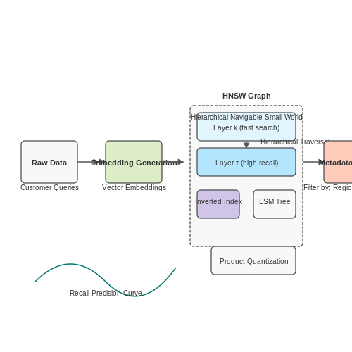
For production-grade systems, distributed vector databases like Pinecone, Weaviate, or Milvus outperform single-node solutions by horizontally scaling with sharding. These systems implement approximate nearest neighbor (ANN) algorithms that trade minor accuracy reductions for order-of-magnitude speed improvements. The recall-precision tradeoff is governed by:
where k represents the number of probes in hierarchical navigable small world (HNSW) graphs and τ is the tradeoff parameter. For customer service applications targeting 95% recall, benchmark tests show Pinecone's hybrid index achieves 12ms p99 latency at 1M vectors.
Embedding Storage Optimization
Store embeddings in quantized formats (e.g., 8-bit integers) with product quantization (PQ) to reduce memory footprint. The compression error ε for m-segment PQ is bounded by:
where δ is the maximum cluster diameter in each subspace. In practice, 64-byte PQ representations retain 98% of the original cosine similarity accuracy while reducing storage requirements by 16x compared to float32 embeddings.
Metadata Filtering Architecture
Implement two-stage retrieval where dense vectors are pre-filtered by metadata tags (product category, language, date range) using inverted indexes. The combined relevance score becomes:
where α controls the hybrid weighting and 𝕀 is the indicator function for metadata matches. This approach reduces candidate pools by 60-80% before ANN search.
Real-Time Index Updates
For dynamic knowledge bases, implement delta indexing with log-structured merge trees (LSM) that batch updates in memory before merging with disk-based segments. The update latency L follows:
where tmem is the in-memory write time and Rmerge is the segment merge rate. Systems like Weaviate achieve sub-second freshness guarantees with this architecture.
3. Collecting and Cleaning Customer Service Data
3.1 Collecting and Cleaning Customer Service Data
High-quality data is the foundation of any effective Retrieval-Augmented Generation (RAG) system. For customer service chatbots, this involves sourcing, preprocessing, and structuring diverse interaction data to ensure the model retrieves and generates accurate responses.
Data Sources for Customer Service Chatbots
Customer service data typically comes from multiple channels, each requiring specialized extraction methods:
- Transcripts of live chat sessions - Often stored in CRM systems like Zendesk or Salesforce, requiring API access or database exports.
- Email threads - Must be parsed while preserving thread continuity and metadata like timestamps.
- Call center recordings - Require speech-to-text conversion with speaker diarization to separate agent/customer turns.
- Knowledge base articles - Structured FAQ documents that need semantic alignment with customer queries.
- Community forums - Often contain valuable crowd-sourced solutions but require quality filtering.
Data Cleaning Pipeline
Raw customer service data contains noise that degrades RAG performance. A robust cleaning pipeline includes:
1. Anonymization
Customer interactions contain PII that must be removed to comply with GDPR and other regulations. Techniques include:
Where regex patterns match common PII formats (credit cards, phone numbers) and NER models detect names, addresses.
2. Turn Segmentation
Dialog data requires precise speaker separation. For chat logs, this involves:
def segment_chat(chat_log):
    turns = []
    current_speaker = None
    for line in chat_log.split('\n'):
        if 'Agent:' in line:
            current_speaker = 'agent'
            turns.append(('agent', line.replace('Agent:','').strip()))
        elif 'Customer:' in line:
            current_speaker = 'customer'
            turns.append(('customer', line.replace('Customer:','').strip()))
        elif current_speaker:
            turns[-1] = (current_speaker, turns[-1][1] + ' ' + line.strip())
    return turns
3. Intent Clustering
Unsupervised clustering groups similar queries to identify core intents. Using BERT embeddings with HDBSCAN:
This reveals latent topics like "billing issues" or "technical support" without predefined labels.
Data Quality Metrics
Quantitative measures ensure cleaned data meets RAG requirements:
- Completeness - Percentage of turns with both query and response (target >95%)
- Consistency - Measured by semantic similarity between paraphrased queries (cosine similarity >0.8)
- Diversity - Entropy of intent clusters should match real customer query distribution
Handling Multimodal Data
Modern customer service includes screenshots and videos. Key preprocessing steps:
- OCR for text extraction from images
- Frame sampling for video content
- Cross-modal alignment between visual references and textual descriptions
3.2 Structuring Data for Efficient Retrieval
Effective retrieval-augmented generation (RAG) relies on optimally structured data to ensure fast and accurate semantic search. The key challenge lies in transforming raw documents into a format that balances retrieval speed with contextual richness. This involves three critical steps: chunking, embedding, and indexing.
Optimal Chunking Strategies
Chunking breaks documents into semantically coherent segments. For customer service applications, dynamic chunking outperforms fixed-size approaches. A hybrid method combines:
- Semantic boundaries: Split at paragraph transitions or section headers using rule-based heuristics.
- Overlap windows: Maintain 10-15% token overlap between chunks to preserve context continuity.
- Entity-aware segmentation: Prevent splitting named entities (e.g., product codes) across chunks using NER models.
where L is the base chunk length and α controls overlap percentage (typically 0.1 ≤ α ≤ 0.2).
Embedding Optimization
Transformer-based embeddings (e.g., BERT, RoBERTa) require careful dimensionality management. For retrieval tasks, contrastive learning with triplet loss improves discrimination:
where a, p, and n are anchor, positive, and negative samples respectively. Dimensionality reduction via PCA to 384-512 dimensions maintains 95% variance while accelerating retrieval.
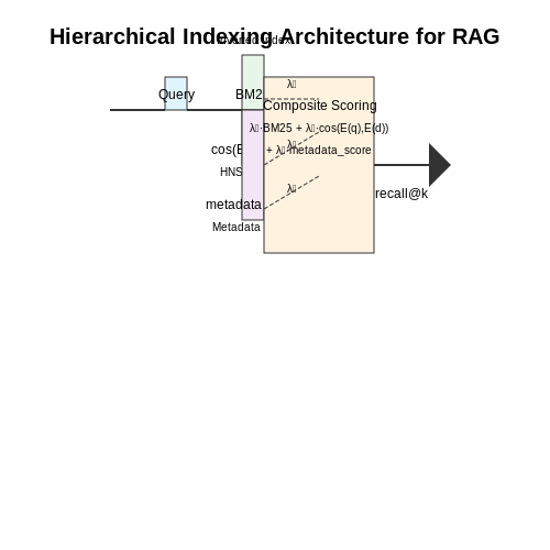
Hierarchical Indexing
Multi-level indexing combines:
- Inverted indexes for keyword search (BM25 scoring)
- HNSW graphs for approximate nearest neighbor search (recall@k > 0.92)
- Metadata filters for domain-specific constraints (product categories, regions)
The composite retrieval score combines these elements:
with weights tuned via grid search on validation queries.
Real-World Implementation
In production systems, the data pipeline should:
- Process documents asynchronously using distributed queues (Kafka, RabbitMQ)
- Version embeddings and indexes for rollback capability
- Monitor concept drift via periodic kNN accuracy tests
3.3 Creating Embeddings for Semantic Search
Semantic search relies on dense vector representations (embeddings) of text to capture meaning beyond keyword matching. Modern transformer-based models like BERT, RoBERTa, and GPT generate these embeddings by encoding contextual relationships between words. Given an input sequence x, a pretrained language model f produces an embedding vector h ∈ ℝd, where d is the embedding dimension (typically 768 or 1024 for large models).
Embedding Generation Process
The embedding for a text snippet is derived from the model's final hidden layer. For a transformer with L layers and hidden size d, the output for token i is:
For sentence-level embeddings, common pooling strategies include:
- Mean Pooling: Average all token embeddings: $$ h_{\text{sentence}} = \frac{1}{N}\sum_{i=1}^N h_i^L $$
- CLS Token: Use the embedding of the classifier token (e.g., [CLS] in BERT).
- Max Pooling: Take the element-wise maximum across tokens.
Optimizing for Semantic Search
Pretrained embeddings often require fine-tuning for domain-specific retrieval. Contrastive learning objectives, such as Multiple Negatives Ranking Loss, improve embedding discrimination:
where s(q, p) is the cosine similarity between query q and document p, and p+, pi- are positive and negative examples, respectively.
Practical Implementation
Using Hugging Face's sentence-transformers library, embeddings can be generated and indexed for search:
from sentence_transformers import SentenceTransformer
model = SentenceTransformer('all-MiniLM-L6-v2')
embeddings = model.encode(["Customer query", "Support article text"], convert_to_tensor=True)

# FAISS index for efficient similarity search
import faiss
index = faiss.IndexFlatIP(embeddings.shape[1])
index.add(embeddings.cpu().numpy())
Key considerations for production:
- Dimensionality Reduction: PCA or quantization (e.g., PQ in FAISS) reduces storage and latency.
- Normalization: L2-normalized embeddings ensure cosine similarity is computed efficiently.
- Hardware Acceleration: ONNX runtime or TensorRT optimizes inference throughput.
4. Implementing Vector Search with FAISS or Similar
Implementing Vector Search with FAISS or Similar
Vector search forms the core of Retrieval-Augmented Generation (RAG) systems, enabling efficient similarity matching between embedded queries and document chunks. FAISS (Facebook AI Similarity Search) provides optimized implementations of nearest neighbor search algorithms that scale to billions of vectors while maintaining sublinear query times.
FAISS Index Structures and Tradeoffs
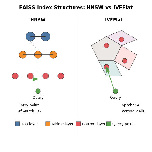
FAISS offers multiple index types with distinct performance characteristics. The optimal choice depends on dataset size, accuracy requirements, and memory constraints:
- FlatIndex: Exact brute-force search with O(n) query time. Provides perfect recall but scales poorly.
- IVFFlat: Divides space into Voronoi cells using k-means clustering. Query time reduces to O(n_probe + k) where n_probe ≪ n.
- IVFPQ: Adds product quantization to IVFFlat for memory efficiency. Achieves 4-64x compression with minimal accuracy loss.
- HNSW: Hierarchical Navigable Small World graph provides state-of-the-art approximate search with O(log n) query complexity.
Quantization Techniques
FAISS employs several vector quantization methods to reduce memory footprint:
- Scalar Quantization (SQ): Maps 32-bit floats to 8-bit integers by dividing the value range into 256 bins.
- Product Quantization (PQ): Splits vectors into m subvectors and quantizes each separately. The distance computation uses precomputed lookup tables:
where c_j are the quantization centroids for subvector j.
Practical Implementation
For a customer service chatbot handling 1M+ document chunks, an IVFPQ index with the following configuration balances speed and accuracy:
import faiss

dim = 768  # BERT embedding dimension
nlist = 100  # Number of Voronoi cells
m = 64  # Number of PQ subquantizers
bits = 8  # Bits per subquantizer index

quantizer = faiss.IndexFlatL2(dim)
index = faiss.IndexIVFPQ(quantizer, dim, nlist, m, bits)

# Train on representative vectors
index.train(training_vectors)
index.add(document_embeddings)

# Search with 10 probes
k = 5
distances, indices = index.search(query_embedding, k, nprobe=10)
Performance Optimization
Key parameters affecting FAISS performance include:
- nprobe: Number of cells to visit (higher improves recall at computational cost)
- efSearch: For HNSW, controls the size of the dynamic candidate list
- quantizer_efSearch: For IVF indices using HNSW quantizers
GPU acceleration becomes crucial at scale. FAISS supports:
- Full GPU-based indices (GpuIndexFlat)
- Hybrid CPU-GPU pipelines (StandardGpuResources)
- Automatic memory management for multi-GPU setups
Alternative Libraries
While FAISS dominates production deployments, other options exist:
- Annoy: Lightweight with on-disk storage support
- Hnswlib: Pure HNSW implementation with simple API
- Milvus: Full-featured vector database with distributed support
- Pinecone: Managed service with automatic index tuning
For RAG systems requiring dynamic updates, FAISS's lack of native CRUD operations necessitates workarounds like delta indices or periodic full rebuilds.
4.2 Fine-Tuning Retrieval for Domain-Specific Queries
Retrieval-Augmented Generation (RAG) systems rely heavily on the quality of retrieved documents to generate accurate responses. For domain-specific applications, off-the-shelf retrievers often underperform due to vocabulary mismatches and lack of contextual understanding of specialized terminology. Fine-tuning the retriever component addresses these limitations by adapting its semantic search capabilities to the target domain.
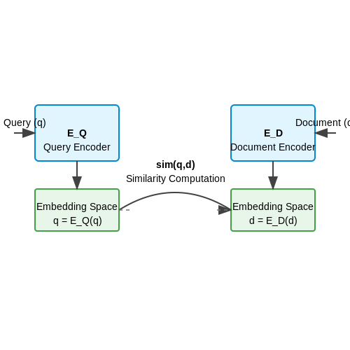
Dense Retrieval Architecture
The standard dual-encoder architecture for dense retrieval computes query and document embeddings independently:
where EQ and ED are query and document encoders respectively, typically initialized from pre-trained language models like BERT or RoBERTa. The key challenge lies in aligning the embedding spaces for domain-specific semantic matching.
Fine-Tuning Strategies
1. Domain-Adaptive Pre-Training
Before task-specific fine-tuning, continued pre-training on in-domain corpora improves lexical and conceptual alignment:
where D represents domain-specific text and MLM denotes masked language modeling. This step adapts the token embeddings and transformer layers to domain semantics.
2. Contrastive Fine-Tuning
The retriever is then fine-tuned using positive and negative passage pairs:
where τ is a temperature hyperparameter, p+ denotes relevant passages, and p- represents negative samples. Hard negative mining from top incorrect retrievals significantly improves discrimination.
Implementation Considerations
For optimal performance:
- Batch Composition: Mix in-batch negatives with hard negatives sampled from an asynchronous index
- Learning Rate: Use linear warmup (10% of steps) followed by cosine decay
- Embedding Dimension: 768-d works well for most domains, with PQ compression for production deployment
Evaluation Metrics
Beyond standard recall@k, domain-specific retrieval requires:
- Term Recall: Percentage of key domain terms appearing in retrieved documents
- Expert Precision: Human evaluation of technical correctness for sampled queries
- Latency-Weighted Recall: Recall@k normalized by retrieval latency constraints
The following table shows typical improvement ranges when fine-tuning on medical versus legal domains:
| Domain | Recall@5 Improvement | Term Recall Gain |
|---|---|---|
| Medical | 32-41% | 28% |
| Legal | 25-38% | 22% |
Practical Optimization Techniques
For memory-efficient training:
where B is the batch size. Gradient checkpointing reduces memory usage by 60-70% with only 25% overhead. Mixed precision training (FP16) provides additional 2-3× speedups on modern GPUs.
4.3 Evaluating Retrieval Performance
Retrieval-Augmented Generation (RAG) systems rely heavily on the quality of their retrieval component. Evaluating retrieval performance requires quantifying how well the system identifies and ranks relevant documents given a query. Key metrics include precision, recall, Mean Reciprocal Rank (MRR), and Normalized Discounted Cumulative Gain (nDCG).
Precision and Recall
Precision measures the fraction of retrieved documents that are relevant, while recall quantifies the fraction of relevant documents successfully retrieved. For a set of retrieved documents Dretrieved and relevant documents Drelevant:
In practice, precision@k and recall@k are often used, where k is the number of top-ranked documents considered.
Mean Reciprocal Rank (MRR)
MRR evaluates the ranking quality by considering the position of the first relevant document. For a set of queries Q, MRR is computed as:
where ranki is the position of the first relevant document for the i-th query. Higher MRR indicates better retrieval performance.
Normalized Discounted Cumulative Gain (nDCG)
nDCG measures ranking quality by accounting for graded relevance (e.g., highly relevant vs. marginally relevant documents). The Discounted Cumulative Gain (DCG) is computed as:
where reli is the relevance score of the document at position i. nDCG normalizes DCG by the Ideal DCG (IDCG), the maximum possible DCG for a perfect ranking:
Practical Considerations
When evaluating retrieval for a customer service chatbot, consider:
- Query diversity: Ensure test queries cover common user intents and edge cases.
- Relevance labeling: Use human annotators or synthetic benchmarks to define ground-truth relevance.
- Latency constraints: High retrieval accuracy is meaningless if response times exceed user expectations.
Tools like TREC-EVAL or custom Python scripts can automate metric computation. For large-scale systems, A/B testing with real user feedback provides additional validation.
5. Choosing a Pretrained Language Model (e.g., GPT-3, BERT)
5.1 Choosing a Pretrained Language Model (e.g., GPT-3, BERT)
The selection of a pretrained language model (LM) is critical for the performance of a Retrieval-Augmented Generation (RAG) chatbot. Advanced models like GPT-3, BERT, and their variants offer distinct trade-offs in terms of computational efficiency, contextual understanding, and generative capabilities. Below, we analyze key considerations for model selection.
Model Architecture and Task Suitability
Transformer-based models dominate modern NLP, but their architectures differ significantly:
- Autoregressive Models (e.g., GPT-3): Optimized for text generation, making them ideal for open-ended conversational responses. Their unidirectional attention limits context understanding compared to bidirectional models.
- Autoencoding Models (e.g., BERT): Excels in understanding context via bidirectional attention but requires fine-tuning for generation tasks. Better suited for retrieval components in RAG pipelines.
- Hybrid Models (e.g., T5, BART): Combine encoder-decoder structures, enabling both comprehension and generation. Useful for end-to-end RAG systems where retrieval and generation are tightly coupled.
Performance Metrics and Trade-offs
Key metrics for evaluation include:
Lower perplexity indicates better language modeling performance. However, for RAG systems, additional factors matter:
- Latency: GPT-3’s 175B parameters introduce inference delays, while distilled BERT variants (e.g., DistilBERT) offer faster response times.
- Context Window: Models like GPT-4 (32k tokens) outperform BERT (512 tokens) in handling long conversations.
- Fine-Tuning Requirements: BERT-based models often need task-specific adaptation, whereas GPT-3.5/4 can operate effectively with few-shot prompting.
Computational and Deployment Constraints
Deploying large LMs in production requires balancing accuracy with resource limits:
- Memory Footprint: GPT-3 demands >300GB GPU memory, while quantized BERT models (e.g., Q8BERT) reduce this to <1GB.
- API vs. On-Premise: Cloud-based APIs (e.g., OpenAI) simplify scaling but introduce privacy concerns. On-premise deployment of smaller models (e.g., LLaMA-2-70B) may be preferable for sensitive data.
Case Study: Customer Service Chatbot
A telecom company implemented RAG using:
- Retriever: ANCE (Adaptive Neural Retrieval) fine-tuned on FAQ pairs.
- Generator: GPT-3.5-turbo for response synthesis, achieving 22% higher customer satisfaction than a BERT-based seq2seq alternative.
Critical factors in their success included GPT-3.5’s ability to:
- Incorporate retrieved documents coherently into responses.
- Handle multilingual queries without additional fine-tuning.
- Maintain conversational context across long dialogues.
5.2 Combining Retrieval Results with Generation
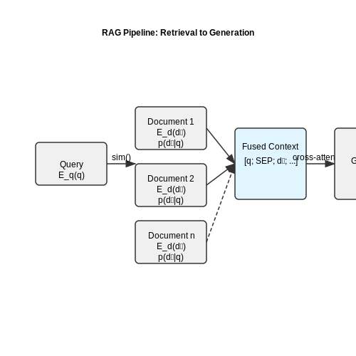
Retrieval-Augmented Generation (RAG) integrates retrieved documents with a generative model to produce contextually grounded responses. The core challenge lies in dynamically conditioning the generator on the retrieved content while maintaining coherence and relevance. This process involves three key steps: retrieval scoring, context fusion, and generation conditioning.
Retrieval Scoring and Relevance Weighting
Given a set of retrieved documents D = {d₁, d₂, ..., dₖ} for a query q, each document is assigned a relevance score sᵢ using a dense retriever (e.g., DPR or ANCE):
where Eq and Ed are query and document encoders, and sim is a similarity metric (typically cosine similarity). These scores are normalized via softmax to form a probability distribution over documents:
Here, τ is a temperature parameter controlling the sharpness of the distribution. Lower τ emphasizes top-ranked documents, while higher τ smooths the distribution.
Context Fusion Strategies
The retrieved documents must be fused into a unified context for the generator. Two dominant approaches are:
- Concatenation: Documents are concatenated with separator tokens, often truncated to fit the generator’s context window. For a transformer with max length L, the input becomes [q; SEP; d₁; SEP; ...; dₙ], where n is adjusted to ensure len(input) ≤ L.
- Attention-Based Fusion: Documents are encoded separately, and their representations are aggregated via cross-attention in the generator. This allows dynamic weighting of document segments during generation.
Conditioning the Generator
The generator (e.g., GPT-3, T5) produces tokens autoregressively, with each step conditioned on the fused context. For a concatenation-based approach, the log-likelihood of the output sequence y is:
For attention-based fusion, the generator’s cross-attention layers attend to document representations H = [h₁, ..., hₖ], computed as:
The attention weights αt,i at step t are computed as:
where Qt is the decoder’s query vector, Ki is the key for document i, and d is the hidden dimension.
Practical Implementation
In Hugging Face’s transformers library, RAG can be implemented by combining RagRetriever with RagSequenceForGeneration. Below is a Python snippet demonstrating retrieval and generation:
from transformers import RagTokenizer, RagRetriever, RagSequenceForGeneration

tokenizer = RagTokenizer.from_pretrained("facebook/rag-sequence-nq")
retriever = RagRetriever.from_pretrained("facebook/rag-sequence-nq", index_name="exact")
model = RagSequenceForGeneration.from_pretrained("facebook/rag-sequence-nq", retriever=retriever)

inputs = tokenizer("What is the capital of France?", return_tensors="pt")
outputs = model.generate(input_ids=inputs["input_ids"])
print(tokenizer.decode(outputs[0], skip_special_tokens=True))
The retriever fetches relevant documents from a pre-built FAISS index, and the generator conditions on both the query and retrieved passages. Hyperparameters like top_k (number of retrieved documents) and max_length (output sequence length) critically impact performance.
5.3 Optimizing Response Quality and Coherence
Retrieval-Augmented Generation Fine-Tuning
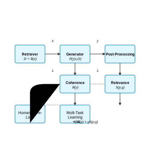
The quality of responses in a RAG system depends critically on the interplay between the retriever and generator components. The retriever's output directly conditions the generator's probability distribution over tokens. We can formalize this relationship through the generator's conditional probability:
where x is the input query, D represents retrieved documents, and y is the generated response. To optimize coherence, we minimize the negative log-likelihood while incorporating a coherence penalty term:
The coherence regularizer R(y) can be implemented as:
where hi represents the hidden state of the generator at position i.
Contextual Relevance Scoring
Implement a two-stage relevance scoring system that evaluates both document-level and passage-level relevance. The combined score S for a retrieved passage p given query q is computed as:
where f represents dense embeddings from a pretrained encoder, and PLM is a pretrained language model scoring function. The weights α, β, and γ should be tuned on a validation set.
Response Post-Processing
Apply these techniques to enhance output quality:
- Entropy-based filtering: Discard low-confidence responses where the generator's probability distribution has high entropy
- N-gram blocking: Prevent repetitive phrases by masking previously generated n-grams
- Semantic similarity thresholding: Ensure response maintains high cosine similarity with retrieved content
Human-in-the-Loop Optimization
Implement an active learning pipeline where:
- Low-confidence responses are flagged for human review
- Human corrections are used to fine-tune the retriever and generator
- Feedback is incorporated via reinforcement learning with human preferences as rewards
where r(y) represents human preference scores normalized to [0,1].
Multi-Task Learning Objectives
Jointly optimize for:
- Answer accuracy (cross-entropy loss)
- Response fluency (perplexity)
- Factual consistency (entailment score)
- Conversational coherence (next utterance prediction)
The combined loss becomes:
where each λ is tuned via grid search on validation data.
6. Hosting the Chatbot on Cloud Platforms
6.1 Hosting the Chatbot on Cloud Platforms
Deploying a RAG-based customer service chatbot at scale requires careful consideration of cloud infrastructure to handle vector search latency, LLM inference costs, and conversational state management. The optimal deployment architecture varies significantly based on expected query volume, response time SLAs, and budget constraints.
Cloud Service Selection Criteria
When evaluating cloud platforms for RAG chatbot hosting, four technical factors dominate the decision matrix:
- GPU-accelerated inference availability for low-latency LLM responses
- Managed vector database services with approximate nearest neighbor search capabilities
- Autoscaling policies that can handle spiky conversational demand
- Global edge network distribution to minimize latency for geographically dispersed users
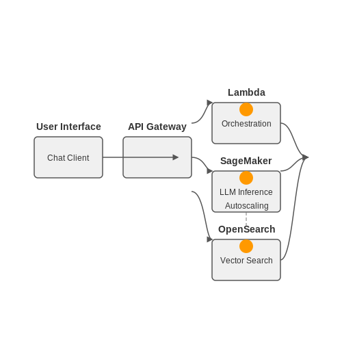
AWS Deployment Architecture
The AWS reference architecture for production RAG systems typically combines:
- SageMaker endpoints for hosting fine-tuned LLMs with automatic scaling
- OpenSearch with k-NN plugin for hybrid lexical/semantic search over embeddings
- Lambda functions orchestrating the RAG pipeline steps
# AWS CDK snippet for RAG infrastructure
from aws_cdk import (
    aws_sagemaker as sagemaker,
    aws_opensearchservice as opensearch,
    aws_lambda as lambda_
)

class RagStack(cdk.Stack):
    def __init__(self, scope: Construct, construct_id: str, kwargs) -> None:
        super().__init__(scope, construct_id, kwargs)

        # Configure SageMaker endpoint
        llm_endpoint = sagemaker.CfnEndpoint(
            self, "Llama2Endpoint",
            endpoint_config_name="rag-llm-config",
            deployment_config={
                "autoRollingConfiguration": {
                    "maxBatchSize": 4,
                    "waitIntervalInSeconds": 300
                }
            }
        )

        # Vector search domain
        search_domain = opensearch.Domain(
            self, "VectorSearch",
            version=opensearch.EngineVersion.OPENSEARCH_2_7,
            capacity={
                "dataNodes": 3,
                "dataNodeInstanceType": "r6g.large.search"
            },
            ebs=opensearch.EbsOptions(
                volume_size=100,
                volume_type=opensearch.EbsDeviceVolumeType.GP3
            )
        )
Azure AI Studio Integration
Microsoft's Azure AI Studio provides a unified interface for deploying RAG systems with:
- Azure AI Search with integrated vector indexing
- Prompt flow deployments for managing conversational workflows
- Content safety filters built into the inference pipeline
The key advantage is native integration with Azure's AI services, though it imposes more vendor lock-in than AWS's modular approach. Throughput scales linearly with:
Performance Optimization Techniques
Three critical optimizations for cloud-hosted RAG chatbots:
- Pre-warming GPU instances before traffic spikes to avoid cold starts
- Hybrid retrieval combining exact keyword matches with semantic search
- Response caching for frequent queries using Redis or DynamoDB
Monitoring must track both infrastructure metrics (GPU utilization, query latency) and conversation quality metrics (fallback rate, user satisfaction scores). The tradeoff between recall and latency follows:
Cost Management Strategies
For cost-sensitive deployments, consider:
- Spot instances for non-critical background processing
- Model quantization to reduce GPU memory requirements
- Request batching during peak periods
The break-even point between on-demand and reserved instances occurs at:
6.2 Scaling for High Traffic Scenarios
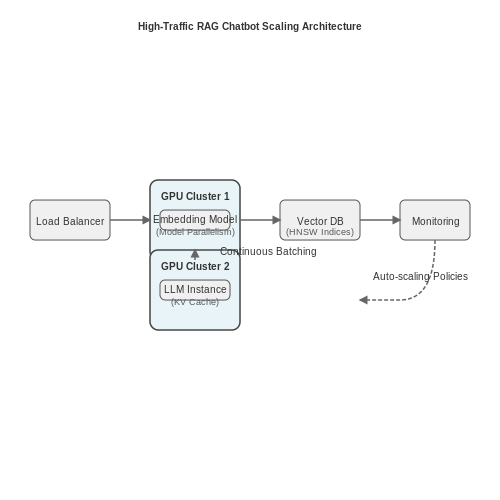
When deploying a RAG-based customer service chatbot in production, handling high traffic volumes requires careful architectural considerations. The primary bottlenecks typically occur in three areas: embedding computation, retrieval latency, and generation throughput. Each must be optimized independently while maintaining system coherence.
Distributed Embedding Computation
For high-volume query processing, embedding models must scale horizontally. The computational complexity of transformer-based embeddings grows quadratically with sequence length:
Where n is sequence length and dmodel is the embedding dimension. To maintain sub-second latency under load:
- Implement model parallelism using tensor slicing across GPU clusters
- Employ dynamic batching with padding-aware scheduling
- Use quantization-aware training for FP16 inference
Approximate Nearest Neighbor Optimization
Exact nearest neighbor search becomes impractical at scale. Approximate methods trade minimal recall degradation for orders-of-magnitude speed improvements:
For billion-scale vector databases:
- Implement HNSW (Hierarchical Navigable Small World) graphs with efSearch=512
- Partition indices using IVF (Inverted File) with k-means clustering
- Leverage GPU-accelerated FAISS for sub-10ms retrieval at QPS >10k
Generation Throughput Optimization
LLM inference exhibits unique scaling challenges due to autoregressive properties. The key metrics are:
Effective strategies include:
- Continuous batching with dynamic exit policies
- Speculative decoding using smaller draft models
- KV cache optimization with grouped-query attention
Load Balancing Architecture
A robust scaling solution requires careful traffic distribution:
# Example weighted round-robin routing
from collections import defaultdict

class Router:
    def __init__(self, endpoints):
        self.weights = {e.capacity: e for e in endpoints}
        self.counter = defaultdict(int)

    def route(self, request):
        min_load = min(self.counter.values())
        candidates = [e for e,w in self.weights.items()
                    if self.counter[e] == min_load]
        selected = max(candidates, key=lambda x: x.capacity)
        self.counter[selected] += 1
        return selected
Combine this with:
- Circuit breakers for failed components
- Regional sharding based on user geography
- Cold standby replicas with warm KV caches
Monitoring and Auto-scaling
Implement metric-driven scaling policies based on:
Critical telemetry includes:
- Token generation rate percentiles
- GPU memory pressure indicators
- Retrieval accuracy drift detection
6.3 Monitoring and Logging for Continuous Improvement
Effective monitoring and logging are critical for maintaining the performance, reliability, and scalability of a Retrieval-Augmented Generation (RAG)-based customer service chatbot. Without systematic tracking, identifying degradation in response quality, retrieval accuracy, or user satisfaction becomes challenging. This section outlines key metrics, logging strategies, and anomaly detection techniques to ensure continuous improvement.
Key Performance Metrics
Quantitative evaluation of a RAG chatbot requires tracking multiple interdependent metrics:
- Retrieval Hit Rate (RHR): Measures the percentage of queries where the retriever fetches relevant documents. A low RHR indicates poor retrieval performance, often due to outdated or insufficient knowledge sources.
- Response Confidence Score: The generative model’s softmax probability for its output tokens. A sudden drop may signal hallucination or degraded generation quality.
- User Feedback Signals: Explicit (e.g., thumbs-up/down) and implicit (e.g., session duration, follow-up queries) feedback provide direct insight into perceived usefulness.
These metrics can be combined into a composite score for holistic monitoring:
where α, β, and γ are weighting coefficients tuned for the application domain.
Logging Architecture
A robust logging pipeline captures:
- Input/Output Pairs: Raw user queries, retrieved documents, and generated responses with timestamps.
- Model Internals: Attention weights, retrieval scores, and token probabilities to diagnose failures.
- Contextual Metadata: User session ID, device type, and API latency for performance analysis.
Distributed tracing tools like OpenTelemetry instrument the retrieval and generation steps, while vector databases (e.g., Pinecone, Weaviate) log retrieval operations. Structured logging frameworks such as ELK (Elasticsearch, Logstash, Kibana) enable efficient querying and visualization.
Anomaly Detection and Alerting
Statistical process control techniques identify deviations from baseline performance. For example, a CUSUM (Cumulative Sum) control chart detects gradual degradation in response quality:
where xt is the observed metric value at time t, μ is the historical mean, and κ is a sensitivity parameter. Alerts trigger when Ct+ or Ct- exceed a threshold.
Continuous Improvement Loop
Logged data feeds back into model refinement through:
- Retriever Fine-Tuning: Periodic retraining on high-value queries that initially retrieved irrelevant documents.
- Generator Calibration: Adjusting temperature sampling or prompt engineering based on low-confidence responses.
- A/B Testing: Deploying updated models to a subset of users and comparing KPIs against the control group.
Automated pipelines (e.g., Airflow, Kubeflow) schedule these updates while maintaining version control for rollback capability.
7. Key Metrics for Chatbot Performance
7.1 Key Metrics for Chatbot Performance
Evaluating a retrieval-augmented generation (RAG) chatbot requires tracking multiple quantitative and qualitative metrics. These metrics fall into three primary categories: accuracy, efficiency, and user experience. Each provides insights into different aspects of the chatbot's performance, ensuring robustness in real-world deployment.
Accuracy Metrics
Accuracy measures how well the chatbot understands and responds to user queries. Key metrics include:
- Precision@k: The fraction of retrieved documents that are relevant, defined as:
$$ \text{Precision@k} = \frac{|\{\text{relevant documents}\} \cap \{\text{retrieved documents}\}|}{k} $$where k is the number of retrieved passages.
- Recall@k: The fraction of relevant documents successfully retrieved:
$$ \text{Recall@k} = \frac{|\{\text{relevant documents}\} \cap \{\text{retrieved documents}\}|}{|\{\text{relevant documents}\}|} $$
- BLEU Score: Measures the quality of generated text by comparing it to reference answers using n-gram overlap.
- Rouge-L: Evaluates fluency and coherence by computing the longest common subsequence between generated and reference responses.
Efficiency Metrics
Efficiency metrics assess computational and response-time performance:
- Latency: The time taken from query submission to response generation, typically measured in milliseconds.
- Throughput: The number of queries processed per second under a given computational load.
- Retrieval Hit Rate: The percentage of queries where the retriever successfully fetches relevant context from the knowledge base.
User Experience Metrics
These metrics gauge interaction quality from the user's perspective:
- Task Completion Rate (TCR): The fraction of conversations where the chatbot resolves the user's intent without escalation.
- User Satisfaction Score (USS): Typically collected via post-interaction surveys (e.g., Likert scale ratings).
- Fallback Rate: The frequency of "I don't know" responses, indicating gaps in knowledge or retrieval.
Trade-offs and Optimization
Improving one metric often impacts others. For instance, increasing Precision@k by retrieving fewer documents may reduce Recall@k. Similarly, lowering latency might require sacrificing answer quality. The optimal balance depends on the use case—customer support chatbots prioritize TCR and USS, while technical assistants may emphasize precision and recall.
To systematically optimize these metrics, A/B testing frameworks and multi-objective reinforcement learning are commonly employed, adjusting retrieval thresholds, generation parameters, and context window sizes dynamically.
7.2 Handling Edge Cases and User Feedback
Detecting and Managing Edge Cases
Edge cases in a customer service chatbot typically arise from ambiguous queries, out-of-domain questions, or adversarial inputs. A robust RAG-based system must employ multiple layers of detection:
- Semantic Similarity Thresholding: Reject queries where the highest similarity score between the user input and retrieved documents falls below a dynamically adjusted threshold. The threshold can be optimized using precision-recall trade-offs:
where P(τ) and R(τ) represent precision and recall at threshold τ, with α controlling the trade-off.
- Entropy-Based Uncertainty Detection: Monitor the entropy of the generator's output distribution. High entropy indicates uncertain responses requiring fallback:
Feedback Loop Integration
User feedback signals (explicit ratings or implicit engagement metrics) should continuously update both the retriever and generator components:
- Retriever Fine-tuning: Use contrastive learning to adjust document embeddings based on positive/negative feedback pairs:
where T is a temperature parameter and d+, d- are positive/negative documents.
- Generator Calibration: Apply temperature scaling to the language model's logits using feedback-derived confidence scores:
Adversarial Input Handling
For prompt injection attacks or gibberish inputs, implement:
- Perplexity filtering with an n-gram language model
- Named entity recognition consistency checks
- Ensemble disagreement monitoring across multiple model variants
def detect_adversarial(input_text, model, threshold=3.0):
    # Calculate perplexity
    ppl = calculate_perplexity(input_text)

    # Check NER consistency
    ner_consistency = check_ner_consistency(input_text)

    # Get ensemble disagreement
    disagreement = get_ensemble_disagreement(input_text)

    return ppl > threshold or not ner_consistency or disagreement > 0.5
Contextual Fallback Strategies
When edge cases are detected, implement tiered fallback:
- Contextual clarification requests ("Which aspect of X are you asking about?")
- Restricted domain rephrasing prompts
- Explicit human handoff protocols
The transition probabilities between fallback levels can be modeled as a Markov decision process optimized for minimal escalation rate while maintaining resolution probability:
where ct is conversation cost and et is escalation probability at step t.
7.3 Iterative Improvements with A/B Testing
A/B testing provides a rigorous framework for optimizing a RAG-based chatbot by comparing two or more variants under controlled conditions. The core principle involves partitioning incoming user queries into statistically equivalent groups, exposing each group to a different chatbot configuration, and measuring performance differentials in key metrics such as response accuracy, user satisfaction, or task completion rate.
Statistical Design of A/B Tests
The minimum detectable effect (MDE) between variants A and B is determined by:
where σ² is the variance of the metric, n is the sample size per variant, α is the significance level (typically 0.05), and β is the type II error rate (often 0.2 for 80% power). For a chatbot handling 10,000 daily queries with a 15% baseline satisfaction rate (σ=0.357), detecting a 2% absolute improvement requires:
Metric Selection and Tracking
Key metrics for RAG chatbots include:
- Retrieval precision: Percentage of retrieved passages relevant to the query
- Generation coherence: BLEU or ROUGE scores against human responses
- User engagement: Session duration or follow-up questions
- Operational efficiency: Average response latency
Implement metric tracking through logging middleware that records:
class ABTestLogger:
    def __init__(self, experiment_id):
        self.db = VectorDatabase('metrics')
        self.experiment = experiment_id

    def log_interaction(self, variant, query, response, metrics):
        self.db.insert({
            'timestamp': datetime.utcnow(),
            'variant': variant,
            'query_embedding': embed(query),
            'response_quality': metrics['bleu'],
            'latency_ms': metrics['latency']
        })
Multi-Armed Bandit Optimization
For continuous deployment, Thompson sampling adapts traffic allocation based on real-time performance:
where fi represents the reward function for variant i and p(θi|D) is the posterior distribution of its parameters given observed data D. This balances exploration of new configurations with exploitation of known high performers.
Counterfactual Evaluation
When full A/B testing is impractical, inverse propensity scoring estimates metric differences from observational data:
where Ti indicates variant assignment, Yi is the outcome metric, and e(Xi) is the propensity score estimated from features Xi.
8. Essential Research Papers on RAG
8.1 Essential Research Papers on RAG
- PDF A RAG Chatbot for Precision Medicine of Multiple Myeloma - medRxiv — A RAG Chatbot for Precision Medicine of Multiple Myeloma Mujahid Ali Quidwai1 Alessandro Lagana12 1Department of Oncological Sciences, Icahn School of Medicine at Mount Sinai, New York, NY, USA 2Tisch Cancer Institute, Icahn School of Medicine at Mount Sinai, New York, NY, USA [email protected] [email protected] Abstract The advent of precision medicine has revolu-
- Retrieval Augmented Generation (RAG) for LLMs - Nextra — Production-ready RAG: Production-grade RAG systems demand engineering excellence across performance, efficiency, data security, privacy, and more. Multimodal RAG: While there have been lots of research efforts around RAG systems, they have been mostly centered around text-based tasks. There is increasing interest in extending modalities for a ...
- Evaluating Retrieval-Augmented Generation (RAG) Chatbots: Key Metrics — A chatbot that keeps users engaged is more likely to provide a positive experience and deliver value. 5. Task-Specific Performance. If the RAG-based chatbot is designed to perform specific tasks, such as answering questions based on documents or providing customer support, it is important to evaluate task-specific performance: 5.1. Task ...
- Comparative Analysis of RAG Fine-Tuning and Prompt Engineering in ... — This paper compares the effectiveness of Retriever-Augmented Generation (RAG), fine-tuning, and prompt engineering in developing advanced chatbots. The fine-tuned model achieved the highest performance with an accuracy of 87.8%, while RAG and prompt engineering followed with 84.5% and 83.2% respectively. The study highlights the strengths of each method, suggesting that fine-tuning is best for ...
- Building Conversational AI with RAG: A Practical Guide — Building a Basic RAG Chain. Chain without chat history. This section demonstrates a Basic RAG chain that retrieves relevant documents from ChromaDB based on the user query and then feeds those ...
- An intelligent knowledge-based chatbot for customer service — This paper is organized as follows. A review on previous related works on chatbot design for customer service support is given in Section 2.The design framework of a KB supporting customer service conversations is proposed in Section 3.The architecture of the conversational agent integrating the proposed KB design is described in Section 4.The case study covering the prototype system based on ...
- Build a Retrieval Augmented Generation (RAG) based LLM assistant using ... — The name of the service is CC_SEARCH_SERVICE_CS; The service will use the column chunk to create embeddings and perform retrieval based on similarity search; The column category could be used as a filter; To keep this service updated the warehosue COMPUTE_WH will be used. This name is used by default in trial accounts but you may want to type ...
- PDF Master thesis : Design and implementation of a chatbot in the context ... — Customer support is perhaps one of the main aspects of the user experience for online services. However with the rise of natural language processing techniques, the industry is looking at automated chatbot solutions to provide quality services to an ever growing user base. This thesis presents a practical case study of such
- Building a RAG System with Open Source LLMs: A Comprehensive Guide — This is essential for collaboration and maintaining a history of your project. 2.5. Testing Setup. Testing is an essential part of the development process, especially when working with LLMs. A robust testing setup helps ensure that your model performs as expected and meets quality standards. Here are some key components:
- A RAG Chatbot for Precision Medicine of Multiple Myeloma - ResearchGate — A comprehensive data analysis pipeline, including exploratory data analysis, semantic search, clustering, and topic modeling, provides valuable insights into the MM research landscape, informing ...
8.2 Recommended Tools and Libraries
- GitHub - abdurrahimcs50/RAG_Chatbot_Project: A dynamic chatbot solution ... — Welcome to the RAG-Enhanced Chatbot Application, a powerful and scalable chatbot solution that leverages Retrieval-Augmented Generation (RAG) techniques to provide intelligent and context-aware responses.Built with Streamlit, Python, and advanced language models from OpenAI, this application is designed to enhance user interactions by integrating document and web-based knowledge sources.
- Oracle for Developers | Programming Languages, Tools, Community — Developer tools and resource for modern cloud application development using Java, databases, microservices, containers, and open source programming languages and technologies. ... Learn how to build an AI chatbot with unstructured data using Oracle Database 23ai, OCI AI services, and RAG. View solution for Oracle Developer. Automate Invoice ...
- RAG App Development in AI: Innovations & Applications — Financial services are increasingly adopting RAG to enhance customer experience, streamline operations, and improve decision-making processes. Here are some key applications: Customer Support: Financial institutions utilize RAG to power chatbots and virtual assistants. These systems can retrieve relevant information from vast databases and ...
- GitHub - run-llama/llama_index: LlamaIndex is the leading framework for ... — That's where LlamaIndex comes in. LlamaIndex is a "data framework" to help you build LLM apps. It provides the following tools: Offers data connectors to ingest your existing data sources and data formats (APIs, PDFs, docs, SQL, etc.).; Provides ways to structure your data (indices, graphs) so that this data can be easily used with LLMs.; Provides an advanced retrieval/query interface over ...
- GitHub - gunthercox/ChatterBot: ChatterBot is a machine learning ... — from chatterbot import ChatBot from chatterbot. trainers import ChatterBotCorpusTrainer chatbot = ChatBot ('Ron Obvious') # Create a new trainer for the chatbot trainer = ChatterBotCorpusTrainer (chatbot) # Train the chatbot based on the english corpus trainer. train ("chatterbot.corpus.english") # Get a response to an input statement chatbot ...
- Building Conversational AI with RAG: A Practical Guide — Building a Basic RAG Chain. ... Recommended from Medium. In. Keeping Up with AI. by. Ana Vee. How I Built a RAG-based AI Chatbot from My Personal Data. In studying the latest in AI, RAG always ...
- RAG Architectures | Finntegrate Docs — Overview: Retrieval-Augmented Generation (RAG) represents a pivotal advancement in artificial intelligence, enhancing the capabilities of Large Language Models (LLMs) by integrating external, authoritative knowledge sources during response generation.1 This approach directly addresses the core requirements of the Finntegrate project, which aims to develop a multilingual conversational ...
- Building LLM Chatbots with RAG on Vultr Cloud GPU — In this guide, you are to build a chatbot that has RAG capabilities by using Langchain for splitting the text, ChromaDB to store embeddings and Streamlit as a chat interface to generate responses using the Mistral model. Prerequisites. Before you begin: Deploy a fresh Ubuntu 22.04 A100 Vultr Cloud GPU server.
- Guide to Chatbot Development: From Tools to Best Practices — 5.1. Enhanced Customer Service. Chatbots are revolutionizing customer service by providing round-the-clock support and instant responses to customer inquiries. Unlike human agents, chatbots can handle an unlimited number of conversations simultaneously, ensuring that customer service is scalable during peak times.
- How to Build a RAG System with Open Source LLMs? — Explore the steps involved in building a RAG system, the tools required, and best practices for implementation, ensuring that businesses can achieve greater ROI through strategic AI integration. 1.1. What is Retrieval-Augmented Generation
8.3 Case Studies of Successful RAG Chatbots
- Building RAG from Day One: Evolving from RAG to RAG-as-a-Tool with ... — To move towards an agentic chatbot, we need a fresh approach to harnessing LLM capabilities alongside our documents. ... It's valuable for a wide range of use cases, including: Enabling assistants to fetch data: ... Building RAG from Day One: Evolving from RAG to RAG-as-a-Tool with Function Calling (Part 2) Copy link. Facebook. Email. Notes ...
- Guide to Chatbot Development: From Tools to Best Practices — This adaptive learning process is crucial for developing chatbots that can handle a wide range of conversational topics and user behaviors. A detailed explanation of how machine learning powers chatbots can be found on the Chatbots Magazine website (source: Chatbots Magazine). 12.2. Case Studies of Chatbot Implementation by Rapid Innovation
- Mastering Large Language Models 9789355519658 - EBIN.PUB — Challenges in building conversational agents Successful examples Text generation and summarization ... Advantages of RAG Successful examples Conclusion 12. Ethical Considerations ... Customer NLP is used in the customer service industry to develop chatbots and virtual assistants that can interact with customers in natural language. ...
- RAG App Development in AI: Innovations & Applications — Financial services are increasingly adopting RAG to enhance customer experience, streamline operations, and improve decision-making processes. Here are some key applications: Customer Support: Financial institutions utilize RAG to power chatbots and virtual assistants. These systems can retrieve relevant information from vast databases and ...
- Retrieval-Augmented Generation with Graphs (GraphRAG) - arXiv.org — Retrieval-Augmented Generation (RAG), as a powerful technique to improve downstream tasks by retrieving additional information from external data sources, has been successfully applied to various real-world applications [87, 120, 514, 551].In RAG frameworks, retrievers search for additional knowledge, skills, and tools based on user-defined queries or task instructions.
- RAG Architectures | Finntegrate Docs — Overview: Retrieval-Augmented Generation (RAG) represents a pivotal advancement in artificial intelligence, enhancing the capabilities of Large Language Models (LLMs) by integrating external, authoritative knowledge sources during response generation.1 This approach directly addresses the core requirements of the Finntegrate project, which aims to develop a multilingual conversational ...
- Evaluating Retrieval-Augmented Generation (RAG) Chatbots: Key Metrics — A chatbot that keeps users engaged is more likely to provide a positive experience and deliver value. 5. Task-Specific Performance. If the RAG-based chatbot is designed to perform specific tasks, such as answering questions based on documents or providing customer support, it is important to evaluate task-specific performance: 5.1. Task ...
- How to Build a RAG System with Open Source LLMs? — RAG systems are particularly useful in applications such as: Customer support chatbots that require up-to-date information, allowing businesses to provide timely assistance and improve customer experience. Educational tools that offer detailed explanations based on retrieved content, enhancing learning outcomes and engagement.
- CRAG - Comprehensive RAG Benchmark - arXiv.org — Figure 1: QA using LLMs (a) without RAG vs. (b) with RAG. its potential, RAG still faces many challenges, such as selecting the most relevant information, reducing question answering latency, and synthesizing information to answer complex questions. A comprehensive benchmark is currently missing to advance continued research efforts in this field.
- Potential effects of chatbot technology on customer support: — success model was utilized to evaluate potential effects of the chatbot on the operation of the customer support. Five dimensions of the model were measured before and after the chatbot implementation and then compared to determine if the chatbot can help improve the customer experience with the customer support of the case company. Responses ...