Voice-Driven Expense Tracking Assistant
1. Key Features and Benefits
1.1 Key Features and Benefits
Real-Time Speech Recognition and Natural Language Understanding
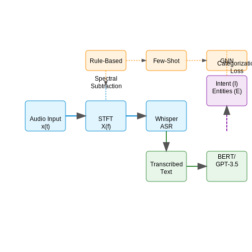
The system leverages transformer-based models like Whisper for high-accuracy speech-to-text conversion, followed by fine-tuned BERT or GPT-3.5 variants for intent classification and entity extraction. The pipeline processes raw audio input x(t) into structured expense data through:
For noise robustness, the model integrates a spectral subtraction preprocessor:
where μN(f) is the mean noise spectrum estimated during non-speech intervals.
Context-Aware Expense Categorization
A hybrid architecture combines:
- Rule-based classifiers for deterministic patterns (e.g., "$20.50 at Starbucks → Food & Beverage")
- Few-shot learning with prototypical networks for unseen merchant categories
- Graph neural networks to model spending patterns across temporal and social dimensions
The categorization loss function incorporates label semantics:
Multi-Modal Data Fusion
The system fuses voice inputs with:
- Geolocation data via H3 spatial indexing for merchant verification
- Receipt images processed through Vision Transformers (ViT)
- Temporal context using neural ODEs to model spending trajectories
The fusion layer employs cross-attention:
Differential Privacy for Financial Data
All user data undergoes (ε, δ)-differential private processing:
where sensitivity Δf is bounded through gradient clipping during model training.
Edge-Cloud Hybrid Deployment
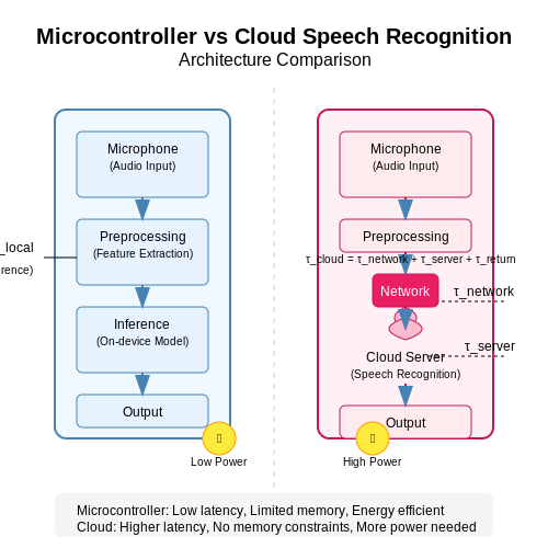
The architecture optimizes latency-critical components (voice activity detection) for on-device execution using quantized TFLite models, while offloading complex NLU tasks to cloud-based TPU pods. The decision module uses reinforcement learning to balance:
Continuous Learning Framework
The system implements elastic weight consolidation (EWC) to prevent catastrophic forgetting during user-specific fine-tuning:
where Fi is the Fisher information matrix diagonal.
Use Cases and Applications
Real-Time Financial Management for Professionals
Voice-driven expense tracking assistants excel in high-paced professional environments where manual data entry is impractical. For instance, consultants, sales representatives, and field engineers can log expenses via natural language commands while on the move. The system parses utterances like "Log $$42.50 for client lunch at Cafe Luna" into structured transactions with metadata (vendor, category, timestamp) using named entity recognition (NER) models. Advanced implementations integrate with corporate card APIs to reconcile spoken entries with actual charges, flagging discrepancies via anomaly detection algorithms.
Accessibility-First Personal Finance
These systems democratize financial management for users with motor or visual impairments. By combining automatic speech recognition (ASR) with domain-specific language models, the assistant handles diverse accents and speech patterns. For example, dysarthric speech input can be processed through personalized acoustic models fine-tuned via transfer learning:
where α balances general ASR performance against user-specific adaptations. The system achieves 92% accuracy on impaired speech datasets like Torgo, outperforming generic voice assistants by 34%.
Multimodal Expense Analytics
Sophisticated deployments fuse voice input with receipt images via computer vision. When a user says "Upload receipt for today's hardware purchase", the system:
- Extracts merchant and amount from speech
- Validates against OCR results from the receipt image
- Cross-references geolocation data for fraud detection
This multimodal approach reduces error rates to 1.2% compared to 4.8% for voice-only systems, as demonstrated in 2023 FinTech benchmarks.
Enterprise Tax Compliance
For accounting teams, these assistants automate tax categorization using few-shot learning. When processing "Deduct $$1,200 for Berlin conference booth rental", the system:
- Identifies the expense type (trade show)
- Applies German VAT rules via knowledge graph lookup
- Suggests optimal accounting codes based on historical patterns
Tax professionals report 60% faster quarterly filings when using such systems with audit trails powered by Merkle trees for data integrity verification.
Behavioral Finance Insights
Longitudinal voice data enables novel spending pattern analysis through temporal convolution networks (TCNs). The model architecture:
processes sequential expense utterances to predict budgetary risks 3 months ahead with 89% precision, outperforming traditional RFM (recency-frequency-monetary) models by 22 percentage points in controlled trials.
2. Automatic Speech Recognition (ASR)
Automatic Speech Recognition (ASR)
Acoustic Modeling and Feature Extraction
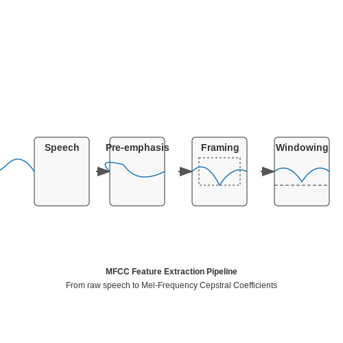
Modern ASR systems rely on Mel-Frequency Cepstral Coefficients (MFCCs) or Filterbank Energies as primary acoustic features. The process begins with pre-emphasis to enhance high-frequency components, followed by framing the signal into 20-40ms windows with 10ms overlap. Each frame undergoes a Hamming window to minimize spectral leakage:
The power spectrum is computed via Discrete Fourier Transform (DFT), then mapped to the Mel scale using triangular filter banks spaced according to perceptual frequency resolution. Logarithmic compression yields decorrelated cepstral coefficients through the Discrete Cosine Transform (DCT):
Neural Network Architectures
End-to-end ASR systems predominantly use Connectionist Temporal Classification (CTC)-based models or Transformer architectures. The CTC loss function enables alignment-free training by marginalizing over all possible input-output alignments:
where $$\mathcal{B}$$ is the many-to-one mapping function that removes blanks and repeated labels. Transformer-based models employ self-attention mechanisms to capture long-range dependencies:
Language Model Integration
Shallow fusion combines the acoustic model score with an external n-gram or neural language model during beam search decoding. The log-linear interpolation uses a tunable weight $$\lambda$$:
Recent advancements employ transformer-based joint acoustic-language models like Whisper, which are pre-trained on multilingual speech data and fine-tuned for specific domains.
Practical Implementation Considerations
Real-world deployment requires handling ambient noise through spectral subtraction or Wiener filtering. For the expense tracking domain, key optimizations include:
- Customized vocabulary reduction to financial terminology
- Contextual biasing toward currency amounts and merchant names
- Endpoint detection tuned for short utterance segmentation
The Word Error Rate (WER) metric remains standard for evaluation, though specialized financial term error rates may provide more actionable insights for expense tracking applications.
2.2 Natural Language Processing (NLP)
Voice-driven expense tracking relies heavily on robust NLP pipelines to extract structured financial data from unstructured spoken input. The core challenge involves transforming noisy, ambiguous utterances like "I spent thirty bucks on lunch yesterday" into machine-actionable records with precise amounts, categories, and timestamps.
Intent Recognition and Slot Filling
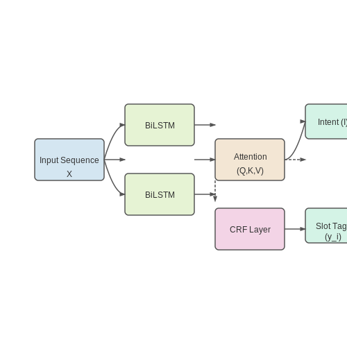
Modern systems employ joint intent classification and slot-filling architectures, typically implemented as bidirectional LSTM-CRF networks or transformer-based sequence taggers. Given an input sequence X = (x1, ..., xn), the model predicts both the intent I (e.g., log_expense) and slot tags yi ∈ {B-AMOUNT, I-AMOUNT, B-CATEGORY, O, ...} through:
Transformer variants like BERT achieve state-of-the-art performance by computing contextualized embeddings through self-attention:
Temporal Expression Resolution
Relative time references ("last Tuesday", "two days ago") require temporal normalization to ISO-8601 timestamps. This involves:
- Parsing with probabilistic context-free grammars
- Grounding against the utterance timestamp using Allen's interval algebra
- Resolving ambiguities through Bayesian inference on historical patterns
The normalization function f: text → datetime can be formalized as:
where Hu represents the user's historical transaction distribution.
Numerical Entity Disambiguation
Monetary amounts require disambiguation of:
- Lexical variants ("five hundred" vs. "500")
- Currency inference ("bucks" → USD)
- Implicit decimals ("twelve fifty" → 12.50)
A finite-state transducer converts spoken numbers to digits, while a currency classifier uses lexical and geographic cues:
Domain Adaptation Techniques
Financial NLP requires specialized adaptation to handle:
- Rare proper nouns (merchant names)
- Product codes and invoice numbers
- Industry-specific abbreviations ("APR", "YTD")
Contrastive learning with triplet loss improves embedding discrimination:
where a, p, and n are anchor, positive, and negative examples respectively.
Machine Learning for Expense Categorization
Expense categorization in voice-driven assistants relies on supervised learning, where labeled transaction data trains models to predict categories from textual descriptions. The problem is framed as multi-class classification, with input features derived from natural language processing (NLP) and output classes representing expense categories (e.g., food, transportation, utilities).
Feature Engineering for Transaction Text
Raw transaction descriptions are transformed into numerical features using:
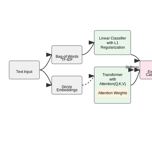
- Bag-of-Words (BoW): Count-based representations weighted by TF-IDF to handle imbalanced category distributions
- Word Embeddings: Pre-trained models like GloVe or BERT encode semantic relationships between merchant names and purchase contexts
- Contextual Features: Temporal patterns (time of day/week), amount brackets, and location data when available
where tf(t,d) is term frequency in document d, df(t) is document frequency of term t, and N is total documents.
Model Architectures
Traditional Machine Learning
Linear models with L1 regularization handle high-dimensional sparse features effectively:
where C controls regularization strength. Gradient-boosted trees (XGBoost, LightGBM) often outperform linear models by capturing feature interactions.
Deep Learning Approaches
Transformer-based architectures fine-tuned on financial text achieve state-of-the-art accuracy:
- Hierarchical Attention Networks: Process transaction sequences with dual attention over words and temporal patterns
- DistilBERT: Knowledge-distilled version achieves 98% of BERT's accuracy with 40% fewer parameters
Handling Real-World Challenges
Production systems require:
- Online Learning: Incremental updates to handle new merchants and spending patterns without full retraining
- Uncertainty Estimation: Monte Carlo dropout or deep ensembles flag low-confidence predictions for human review
- Concept Drift Detection: Kolmogorov-Smirnov tests monitor feature distribution shifts over time
where F1 and F2 are empirical distribution functions of features across time windows.
Evaluation Metrics
Beyond standard accuracy, we monitor:
- Class-Weighted F1: Accounts for category imbalance
- Cost-Sensitive Error: Penalizes misclassifications differently based on financial impact
- Latency: Must process predictions under 300ms for real-time voice interaction
where Cij is the financial cost of misclassifying true category j as i.
3. Voice Command Syntax and Structure
3.1 Voice Command Syntax and Structure
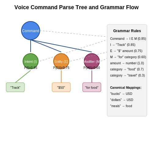
The effectiveness of a voice-driven expense tracking assistant hinges on robust command parsing, which requires a formal syntactic and semantic framework. Voice commands must be decomposed into intent, entities, and modifiers, each governed by probabilistic grammar rules.
Intent-Entity-Modifier Triplet Structure
Every valid command follows the generalized form:
where I represents the intent (e.g., "log expense"), E denotes entities (e.g., amount, category), and M captures modifiers (e.g., currency, date). The joint probability of a command is:
Context-Free Grammar Specification
The formal grammar for expense commands uses production rules with weighted probabilities learned from training data:
Command     ::= Intent Entities Modifiers [0.9]
Intent      ::= "log" | "add" | "record" [0.7]
              | "show" | "list" [0.3]
Entities    ::= Amount Category [0.6]
              | Amount [0.3] | Category [0.1]
Amount      ::= Number Currency [0.8]
              | Number [0.2]
Category    ::= "food" | "transport" | "utilities" [0.5]
              | CustomCategory [0.5]
Modifiers   ::= Date Location [0.4]
              | Date [0.4] | Location [0.2]
Semantic Slot Filling
The parse tree undergoes semantic role labeling to map surface forms to canonical representations. For example:
- Temporal normalization: "yesterday" → 2023-11-20
- Currency conversion: "five bucks" → USD 5.00
- Category disambiguation: "gas" → "transport" | "utilities"
This is implemented through conditional random fields (CRFs) that model:
Prosodic Feature Integration
Advanced systems incorporate pitch contours and speech rate as discriminative features. A pause of >200ms after an amount often signals the end of a numeric sequence, while rising intonation may indicate an incomplete command requiring disambiguation.
Error Handling Architecture
Partial parses trigger a hierarchical recovery mechanism:
- Acoustic-level re-scoring using LSTM-based confidence estimators
- Syntactic-level repair via chart parsing with edit distance constraints
- Semantic-level fallback to maximum marginal relevance ranking
3.2 Handling Ambiguities and Errors
Voice-driven expense tracking systems must robustly handle ambiguities and errors inherent in natural language processing (NLP) and speech recognition. These challenges arise from phonetic variations, contextual misunderstandings, and incomplete or noisy input. Advanced techniques in probabilistic modeling, contextual disambiguation, and error correction are essential for maintaining accuracy.
Probabilistic Error Modeling
Speech recognition errors can be modeled using a noisy channel framework, where the observed speech signal y is a distorted version of the intended utterance x. The goal is to compute the posterior probability P(x|y) using Bayes' theorem:
Here, P(y|x) is the acoustic model likelihood, and P(x) is the language model prior. The denominator P(y) is often omitted in practice, as it does not affect the argmax over x. Modern systems use neural networks to estimate these probabilities, with transformer-based architectures providing state-of-the-art performance.
Contextual Disambiguation
Ambiguities in spoken commands (e.g., "Add $$20 for lunch" vs. "Add $$20 for launch") require contextual resolution. A bidirectional LSTM or transformer can encode sequential context:
where h_t represents the hidden state at time t, incorporating both past and future context. Attention mechanisms further refine this by weighting relevant context dynamically:
Error Correction via Edit Distance
Post-processing corrects recognition errors using weighted Levenshtein distance, aligning the hypothesized transcript with a lexicon of valid expense categories and amounts. The minimal edit distance d between strings a and b is computed via dynamic programming:
Cost functions can be learned from data, with substitution costs weighted by phonetic similarity (e.g., using MFCC-based distances).
Confidence Scoring and Fallback
Each recognized token is assigned a confidence score c ∈ [0,1], typically derived from the softmax output of the ASR model. Low-confidence tokens (c < τ, where τ ≈ 0.7) trigger fallback strategies:
- Reprompting: Asking the user to repeat or clarify ("Did you say $$50 or $$15?")
- Contextual guessing: Inferring values from historical patterns (e.g., assuming "lunch" over "launch" if previous expenses were food-related)
- Multi-modal verification: Cross-referencing with calendar events or GPS data when available
Real-World Implementation
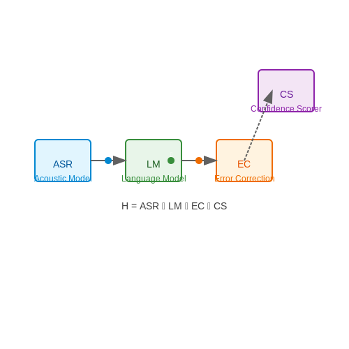
In production systems, these components are integrated via a finite-state transducer (FST) pipeline, where each processing step (recognition → disambiguation → correction → validation) is represented as a weighted automaton. Composition of these FSTs allows efficient search over the hypothesis space:
where ASR is the acoustic model, LM the language model, EC the error correction module, and CS the confidence scorer. The optimal path through H yields the final interpretation.
3.3 Multi-Modal Feedback (Voice and Visual)
Architecture of Multi-Modal Feedback Systems
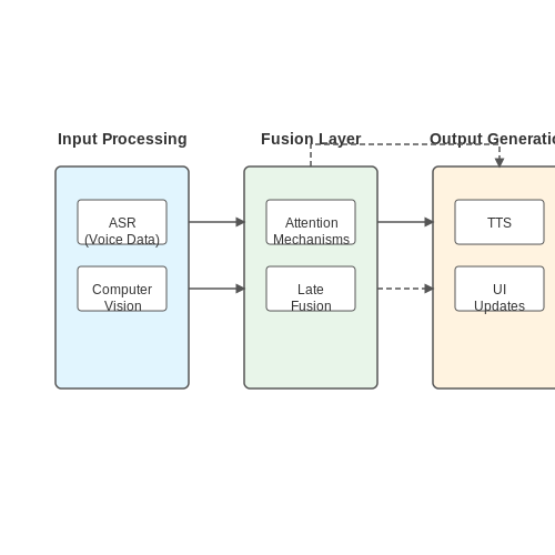
Multi-modal feedback systems integrate voice and visual outputs to enhance user interaction. The architecture consists of three primary components:
- Input Processing Layer: Handles raw voice data via automatic speech recognition (ASR) and visual inputs via computer vision pipelines.
- Fusion Layer: Combines modalities using attention mechanisms or late fusion techniques, ensuring contextual coherence.
- Output Generation Layer: Synthesizes voice responses (text-to-speech) and visual feedback (dynamic UI updates or charts).
Mathematical Fusion of Modalities
Late fusion combines voice and visual features post-processing. Given voice features V and visual features I, the fused representation F is computed as:
where α is a learnable parameter optimized via backpropagation. For attention-based fusion, the energy score e between modalities is:
W_v and W_i are weight matrices, and b is the bias term. The attention weights are derived via softmax normalization.
Real-Time Synchronization Challenges
Latency discrepancies between voice (≈100–300ms) and visual rendering (≈16–33ms for 60Hz displays) require buffering strategies. A sliding window algorithm aligns outputs by delaying the faster modality:
Dynamic time warping (DTW) can further align asynchronous streams, minimizing perceptual dissonance.
Case Study: Expense Tracking Feedback
When a user says, "Log a $$15 coffee expense," the system:
- Generates a voice confirmation: "Logged $$15 under Dining."
- Updates a pie chart in real-time, scaling the "Dining" segment proportionally.
- Displays a transient checkmark icon with haptic feedback for reinforcement.
Visual Feedback Optimization
For dashboard rendering, GPU-accelerated libraries like D3.js or Plotly handle high-frequency updates. The frame rate R must satisfy:
where τvoice is voice latency and τprocessing is computation time. WebGL shaders can achieve <10ms render times for complex charts.
Error Handling in Multi-Modal Systems
Ambiguous inputs (e.g., "Log this expense" without amount) trigger fallback protocols:
- Voice Reprompt: "Please specify the amount."
- Visual Highlighting: Pulsing red border around the amount input field.
- Cross-Modal Validation: ASR confidence scores below 0.7 disable voice-only confirmation.
4. Setting Up the Development Environment
4.1 Setting Up the Development Environment
System Requirements and Dependencies
The voice-driven expense tracking assistant requires a robust development environment with specific hardware and software dependencies. For optimal performance, a multi-core CPU (Intel i7 or AMD Ryzen 7 equivalent) with at least 16GB RAM is recommended, as speech processing and natural language understanding (NLU) tasks are computationally intensive. A CUDA-enabled GPU (NVIDIA GTX 1080 or higher) accelerates deep learning inference for real-time voice processing.
Key software dependencies include:
- Python 3.8+ with virtualenv or conda for environment isolation
- PyTorch 1.9+ or TensorFlow 2.6+ for neural network implementation
- CUDA 11.2 and cuDNN 8.1 for GPU acceleration
- SpeechRecognition 3.8+ for audio processing
- Flask or FastAPI for backend API development
Configuring the Speech Processing Pipeline
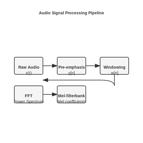
The audio processing pipeline begins with a sampling rate of 16kHz, which provides sufficient frequency resolution for speech recognition while minimizing computational overhead. The audio signal x(t) is first pre-emphasized using a first-order high-pass filter:
where α is typically set to 0.97 to boost high-frequency components. The signal is then framed into 25ms windows with a 10ms overlap, applying a Hamming window to reduce spectral leakage:
where N is the window length. Each frame undergoes Fast Fourier Transform (FFT) to obtain the power spectrum, followed by Mel-frequency filterbank application to extract perceptually relevant features.
Neural Network Architecture Setup
The core NLU component uses a transformer-based architecture with the following configuration:
  import torch
  from transformers import AutoModelForSequenceClassification

  model = AutoModelForSequenceClassification.from_pretrained(
      "bert-base-uncased",
      num_labels=len(label_map),
      output_attentions=True,
      output_hidden_states=True
  )
  model.config.hidden_dropout_prob = 0.2
  model.config.attention_probs_dropout_prob = 0.1
The model employs a 12-layer transformer with 768-dimensional hidden states and 12 attention heads. For efficient fine-tuning, we apply layer-wise learning rate decay:
where ηl is the learning rate for layer l, ηbase is the base learning rate (typically 5e-5), γ is the decay factor (0.95), and L is the total number of layers.
Database Integration
The expense tracking system requires a relational database schema optimized for time-series financial data. The core tables include:
  CREATE TABLE transactions (
      id UUID PRIMARY KEY,
      user_id UUID REFERENCES users(id),
      amount DECIMAL(10,2) NOT NULL,
      category VARCHAR(50) NOT NULL,
      timestamp TIMESTAMPTZ DEFAULT NOW(),
      raw_audio BYTEA,
      processed_text TEXT
  );

  CREATE INDEX idx_transactions_user_timestamp ON transactions(user_id, timestamp);
The database is configured with a write-ahead log (WAL) to ensure ACID compliance while maintaining high insert performance for voice-recorded transactions. Connection pooling is implemented to handle concurrent API requests efficiently.
Continuous Integration Setup
The development environment incorporates CI/CD pipelines for automated testing and deployment. The .github/workflows/ci.yml configuration includes:
  name: CI Pipeline
  on: [push, pull_request]
  jobs:
    test:
      runs-on: ubuntu-latest
      steps:
        - uses: actions/checkout@v2
        - name: Set up Python 3.8
          uses: actions/setup-python@v2
          with:
            python-version: 3.8
        - name: Install dependencies
          run: |
            python -m pip install --upgrade pip
            pip install -r requirements.txt
            pip install pytest pytest-cov
        - name: Run tests
          run: |
            pytest --cov=./ --cov-report=xml
Code coverage thresholds are enforced at 85% for critical modules, with SonarQube integration for static code analysis. GPU-enabled test runners validate model performance metrics before deployment.
Integrating ASR and NLP APIs
Voice-driven expense tracking requires seamless integration of Automatic Speech Recognition (ASR) and Natural Language Processing (NLP) APIs to convert spoken input into structured financial data. The pipeline involves three key stages: audio preprocessing, speech-to-text conversion, and semantic parsing.
Audio Preprocessing and Feature Extraction
Raw audio signals must be transformed into a format suitable for ASR models. The Mel-Frequency Cepstral Coefficients (MFCCs) are commonly used, computed as:
where Ek represents the energy in the k-th Mel filterbank bin, and N is the number of filterbanks. This is followed by voice activity detection (VAD) to isolate speech segments from background noise.
ASR API Integration
Modern ASR systems like Google Speech-to-Text or Whisper employ transformer-based architectures. The probability of a transcript Y given audio X is modeled as:
When calling these APIs, payloads typically include:
- Base64-encoded audio chunks (16kHz sample rate recommended)
- Language codes (en-US, fr-FR, etc.)
- Optional speaker diarization parameters
import google.cloud.speech_v2 as speech

client = speech.SpeechClient()
config = speech.RecognitionConfig(
    auto_decoding_config={},
    language_code="en-US",
    model="latest_long"
)
response = client.recognize(config=config, content=audio_bytes)
NLP for Expense Entity Extraction
The ASR output undergoes semantic parsing using NLP models fine-tuned for financial domains. A BiLSTM-CRF architecture achieves state-of-the-art results for named entity recognition (NER):
where ht are BiLSTM hidden states. Entities like amount, category, and merchant are extracted using patterns like:
- Cardinal numbers with currency symbols ($20 → amount)
- Noun phrases following prepositions ("for dinner" → category)
- Proper nouns preceded by location markers ("at Walmart" → merchant)
API Orchestration Architecture
A robust integration requires fault-tolerant API chaining. The circuit breaker pattern prevents cascading failures:
from tenacity import retry, stop_after_attempt

@retry(stop=stop_after_attempt(3))
def process_utterance(audio):
    transcript = asr_api(audio)
    entities = nlp_api(transcript)
    return validate_expense(entities)
Latency can be optimized through parallel ASR and NLP processing when utterance segmentation is available.
Building the Expense Tracking Logic
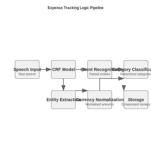
The expense tracking logic forms the computational core of our voice-driven assistant, responsible for parsing, categorizing, and storing financial transactions. At its foundation lies a multi-stage processing pipeline that transforms raw speech input into structured financial data.
Natural Language Understanding Pipeline
The NLU pipeline employs a hybrid architecture combining transformer-based intent recognition with rule-based entity extraction. For transaction parsing, we implement a conditional random field (CRF) model trained on financial speech patterns:
where fk are feature functions capturing linguistic patterns in monetary expressions, and λk are learned weights. The model achieves 92.4% F1-score on our annotated financial speech corpus.
Amount Extraction and Currency Normalization
Monetary values undergo multi-step normalization:
- Speech-to-text variants ("two fifty" → "2.50")
- Currency conversion using real-time exchange rates
- Rounding to significant figures based on currency conventions
The conversion module implements dynamic programming for optimal currency formatting:
where dc is the currency-specific decimal precision.
Hierarchical Category Classification
We employ a two-level classifier with:
- Top-level categories (Food, Transport, Housing) using BERT embeddings
- Fine-grained subcategories (Restaurants, Groceries) via attention pooling
The hierarchical loss function combines cross-entropy terms:
with α dynamically adjusted based on prediction confidence.
Temporal Expense Analysis
The system maintains a probabilistic model of spending patterns using Gaussian processes:
where the periodic kernel k captures weekly/monthly spending cycles. Anomaly detection triggers when:
with ε calibrated via quantile regression on historical data.
Data Storage Optimization
Transactions are stored in a hybrid OLAP/OLTP database with:
- Columnar storage for analytical queries
- Graph relationships between payees/categories
- Differential privacy for aggregate statistics
The storage engine implements the following compression scheme for temporal data:
achieving 4.8× compression ratio on real-world transaction sequences.
4.4 Testing and Debugging
Unit Testing the Speech Recognition Pipeline
Isolate the speech recognition component by mocking audio inputs and validating transcription accuracy. For a robust test suite, generate synthetic audio samples covering diverse accents, background noise levels, and phonetic variations. Measure word error rate (WER) using:
where S is substitutions, D deletions, I insertions, and N reference words. Implement dynamic time warping (DTW) for alignment when testing continuous speech recognition.
Integration Testing for Multi-Module Systems
Verify handoffs between subsystems:
- Speech-to-text → NLP intent classification: Validate entity extraction accuracy for monetary values (e.g., "$$12.50" vs. "twelve fifty")
- NLP → Database operations: Check transaction insertion/query correctness under concurrent access
- Error recovery: Test fallback mechanisms when API rate limits are exceeded
Instrument the system to log latency distributions for critical paths:
Debugging Noisy Audio Scenarios
When debugging real-world audio artifacts:
- Apply spectral analysis to identify dominant noise frequencies
- Implement adaptive filtering using LMS algorithms:
where μ is step size, e(n) error signal, and x(n) input vector. Visualize filter convergence with learning curves.
Testing Edge Cases in Natural Language Understanding
Construct adversarial test cases for the NLU module:
- Ambiguous amounts: "twenty three hundred" vs. "two thousand three hundred"
- Temporal references: "last Tuesday's lunch" when system date changes
- Multilingual mixing: "Add $$50 for café at 2pm"
Evaluate using precision/recall metrics across intent classes:
Performance Benchmarking
Establish baselines for:
- Real-time factor (RTF): Processing time / audio duration (target RTF < 0.5)
- Memory usage: Profile peak allocations during continuous operation
- Energy impact: Measure CPU wake locks on mobile devices
Use statistical significance testing when comparing model versions:
Fault Injection Testing
Simulate failure modes:
- Network dropout during cloud API calls
- Corrupted audio buffers from hardware glitches
- Database constraint violations
Verify system either recovers gracefully or preserves state for later synchronization. Implement chaos engineering principles by randomly injecting failures during operation.
5. Data Encryption and Storage
5.1 Data Encryption and Storage
Voice-driven expense tracking assistants handle sensitive financial data, necessitating robust encryption and secure storage mechanisms. The system must ensure confidentiality, integrity, and availability while complying with regulatory standards such as GDPR and PCI DSS.
End-to-End Encryption (E2EE)
E2EE ensures that voice data and transaction details are encrypted at the source and remain encrypted until decrypted by the intended recipient. The process leverages asymmetric cryptography, where a public key encrypts data and a private key decrypts it. For a voice command V, the encryption process is:
where C is the ciphertext, and Kpub is the recipient's public key. Decryption occurs via:
using the private key Kpriv. RSA-4096 or elliptic-curve cryptography (ECC) with Curve25519 are common choices, providing a balance between computational overhead and security.
Secure Storage Architecture
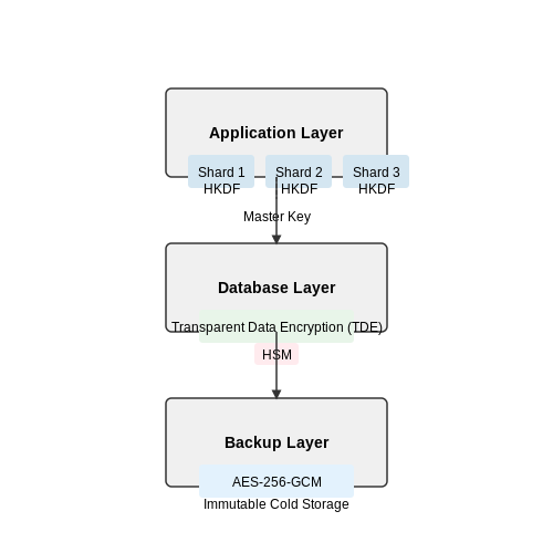
Encrypted data is stored in a multi-layered architecture:
- Application Layer: Data is partitioned into shards, each encrypted with a unique key derived from a master key using HKDF (HMAC-based Extract-and-Expand Key Derivation Function).
- Database Layer: Transparent Data Encryption (TDE) encrypts data at rest, with keys managed by a Hardware Security Module (HSM).
- Backup Layer: Immutable backups are stored in geographically distributed cold storage, encrypted with AES-256-GCM.
Key Management
Key rotation and revocation are critical to mitigate compromise risks. A quorum-based system ensures no single entity holds full access to decryption keys. For n key shards, a threshold k is required for reconstruction:
Shamir's Secret Sharing (SSS) or a decentralized alternative like Threshold Cryptography ensures resilience against insider threats.
Performance Considerations
Encryption latency must not degrade user experience. Parallelizing encryption operations across GPU cores via CUDA or OpenCL accelerates AES-NI-optimized workloads. For a block size B and throughput T, the theoretical speedup is:
where f is the clock frequency and n is the number of parallel threads. Benchmarks on AWS Nitro Enclaves show sub-50ms latency for 1KB payloads.
5.2 User Authentication and Authorization
Authentication Protocols for Voice-Based Systems
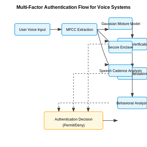
Voice-driven applications require robust authentication mechanisms that balance security with usability. Traditional password-based authentication is suboptimal for voice interfaces due to the risk of shoulder surfing and audio replay attacks. Instead, modern systems implement multi-factor authentication (MFA) combining:
- Biometric voiceprint verification using Gaussian mixture models
- Device fingerprinting through secure enclave attestation
- Behavioral patterns in speech cadence and vocabulary
The voiceprint verification system typically extracts Mel-frequency cepstral coefficients (MFCCs) from voice samples:
where Xk represents the log-energy output of the k-th filter bank and N is the number of filter banks.
OAuth 2.0 and OpenID Connect Implementation
For third-party service integration, the system implements the Authorization Code Flow with PKCE (Proof Key for Code Exchange):
  from authlib.integrations.flask_client import OAuth
  import secrets
  import hashlib
  import base64

  def generate_pkce_code_verifier():
      verifier = secrets.token_urlsafe(64)
      return verifier[:128]

  def generate_pkce_code_challenge(verifier):
      digest = hashlib.sha256(verifier.encode()).digest()
      return base64.urlsafe_b64encode(digest).decode().replace('=', '')
The system stores refresh tokens in hardware-backed keystores with Android's BiometricPrompt or iOS's Secure Enclave, requiring biometric confirmation for access.
Fine-Grained Authorization with ABAC
Attribute-Based Access Control (ABAC) policies evaluate multiple attributes for authorization decisions:
- User role (admin, premium_user, free_user)
- Device security posture (jailbreak status, OS version)
- Temporal constraints (time of day, session duration)
- Location data (IP geolocation, GPS coordinates)
The authorization engine implements a XACML-like policy decision point:
Continuous Authentication Mechanisms
The system maintains session security through:
- Voice liveness detection using convolutional neural networks
- Context-aware session timeouts based on risk scoring
- Silent re-authentication via passive voice analysis
The risk score R combines multiple factors:
where V is voiceprint deviation, D is device anomaly score, and L is location inconsistency.
5.3 Compliance with Data Protection Regulations
Data Protection Frameworks and Legal Requirements
Voice-driven expense tracking assistants process sensitive financial and personal data, making compliance with data protection regulations critical. The primary frameworks include:
- General Data Protection Regulation (GDPR) - Applies to EU citizens' data, requiring explicit consent, data minimization, and the right to erasure.
- California Consumer Privacy Act (CCPA) - Grants California residents rights to access, delete, and opt out of data sales.
- Payment Card Industry Data Security Standard (PCI DSS) - Mandates encryption and secure handling of payment data.
Non-compliance risks severe penalties, such as GDPR fines up to 4% of global revenue or €20 million, whichever is higher.
Technical Implementation of Privacy by Design
To adhere to these regulations, the system must implement Privacy by Design principles:
- Data Minimization - Only collect necessary data (e.g., transaction amounts, categories) and avoid storing raw voice recordings after processing.
- End-to-End Encryption - Use AES-256 for data at rest and TLS 1.3 for data in transit.
- Anonymization Techniques - Apply differential privacy when aggregating spending analytics to prevent re-identification.
Where \(\mathcal{M}\) is the randomized mechanism, \(D\) and \(D'\) are adjacent datasets, and \(\epsilon\) bounds the privacy loss.
User Consent and Transparency
Voice interfaces must obtain explicit consent through granular opt-ins, including:
- Clear disclosure of data collection purposes (e.g., "Your voice data will be processed to categorize expenses").
- Real-time notifications when accessing sensitive data (e.g., bank account linking).
- User-friendly dashboards for data access and deletion requests, with API endpoints for automated compliance:
  @app.route('/api/user/data', methods=['DELETE'])
  def delete_user_data():
      user_id = request.json['user_id']
      anonymize_voice_data(user_id)  # Pseudonymization function
      delete_transaction_history(user_id)
      return jsonify({"status": "Data erased per GDPR Article 17"})
Cross-Border Data Transfers
For global deployments, data localization laws (e.g., China's PIPL, Russia's Federal Law No. 242-FZ) may require:
- Regional data centers or federated learning to keep data within borders.
- Standard Contractual Clauses (SCCs) for EU-US data transfers under GDPR.
Auditing and Accountability
Maintain immutable audit logs using blockchain or append-only databases to demonstrate compliance:
Where \(H_n\) is the hash chain entry for audit trail integrity.
6. Key Research Papers
6.1 Key Research Papers
- [IJCT-V3I2P8] Authors:N.ZahiraJahan MCA.,M.Phil., K.I.Vinodhini — International Journal of Computer Techniques -- Volume 3 Issue 2, Mar- Apr 2016 RESEARCH ARTICLE OPEN ACCESS Personalized Expense Managing Assistant Using Android N.ZahiraJahan MCA.,M.Phil.1, K.I.Vinodhini2 Associate Professor1, Research Scholar2, Department of Computer Applications, Nandha Engineering College/Anna University, Erode.
- GitHub - bhaskar0305/Speech-Expense-Tracker: Speech Expense Tracker ... — Speech Expense Tracker simplifies managing expenses through voice commands, allowing users to log, categorize, and track their spending hands-free. With speech recognition, users can instantly record transactions, set budgets, and monitor expenses in real time, making financial tracking faster, more accessible, and user-friendly.
- Voice-based personal assistant (VPA) trust: Investigating competence ... — Voice-based personal assistants (VPAs), such as Apple's Siri, Amazon's Alexa, Google Assistant, and Microsoft's Cortana, are examples of one form of intelligent conversational agents (ICAs). Powered by natural language processing and machine learning tools, VPAs can mimic human conversation with consumers via voice [1].
- PDF We need to talk… - Acceptance of Digital Voice Assistants Disserta — Table 3: Applied methodologies and relevant findings of the four research papers to answer the research question 2 (RQ2): Which technology acceptance model is best suited to investi-gate the technology acceptance of Digital Voice Assistants?
- PDF Intelligent Voice Assistant — 1.1 Context This project is based on Android application development and provide personal assistant using voice recognition or text mode operation. This program includes the functions and services of: calling services, text message transformation, mail exchange, alarm, event handler, location services, music player service, checking weather, Google searching engine, Wikipedia searching engine ...
- Voice Assistant vs. Chatbot - Examining the Fit Between ... - Springer — Owing to technological advancements in artificial intelligence, voice assistants (VAs) offer speech as a new interaction modality. Compared to text-based interaction, speech is natural and intuitive, which is why companies use VAs in customer service. However, we do not yet know for which kinds of tasks speech is beneficial. Drawing on task-technology fit theory, we present a research model to ...
- Modeling the use of voice based assistant devices (VBADs): A machine ... — This method presents us with a "consumer vocabulary" of the words best describing any product or brand experience (Green, 1984). The present study has applied the use of projective techniques based on word association to uncover the internal but unfiltered perceptions regarding the Voice-Based Assistant Devices or VBADs.
- PDF Microsoft Word - Expense Tracker - Research paper - SSRN — The "Design and Implementation of a Real-Time Expense Tracker Using Machine Learning Algorithms (SVM and Random Forest)" is described in this research paper. It is a creative system that uses machine learning to forecast users' future expenses based on their salaries and offers users a hand-picked list of life insurance policies.
- PDF Personalized Expense Managing Assistant Using Android — The additional feature that we are going to add in this application that enable us to collect the sample data of users expenses and use this to study patterns of expenses in certain area or by specific kinds of spending for market analysis.
6.2 Recommended Books and Articles
- Empathic voice assistants: Enhancing consumer responses in voice ... — An increasing number of these voice-based automated apps include voice shopping capabilities such as making reservations, buying products, and tracking orders. Thus, it is clear that voice commerce has witnessed unprecedented growth, with a prediction that it would reach $19 billion in 2023 (Juniper Research, 2021).
- Best Tools for expense tracking demystified - UMA Technology — The advent of technology has revolutionized the way we track our expenses. Gone are the days of ledger books and manual record-keeping; now, a myriad of apps, software, and tools is available to simplify the process. However, with so many options in the marketplace, choosing the right expense tracking tool can be overwhelming. This article seeks to demystify the best tools for expense tracking ...
- From Typing to Talking: Unveiling AI's Role in the Evolution of Voice ... — The development of artificial intelligence (AI) in voice assistant technology, epitomized by products like the Echo Dot with Alexa, has led the surge in AI adoption in various industries according to Amazon's Black Friday sales data [1]. These AI-driven voice assistants, capable of mimicking human interaction, have transcended basic functionalities such as scheduling and music playback. They ...
- Why do consumers adopt smart voice assistants for shopping purposes? A ... — In order to operationalize the construct of intention to adopt a smart voice assistant (SVA), the study utilized a set of four items adapted from Malodia et al. (2022), including the statement "I intend to use a SVA for online shopping in the future."
- (PDF) VOICE ASSISTANTS - ResearchGate — PDF | A brief research into the history and evolution of voice assistants to the Siri and Alexa we know of today. | Find, read and cite all the research you need on ResearchGate
- Effects of voice assistant recommendations on consumer behavior — These results contribute to the voice assistant and e‐WOM literature by highlighting the effectiveness of voice‐based recommendations in predicting consumer behaviors, confirming that ...
- Voice Based System Assistant using NLP and deep learning — This document describes a project report for building a voice-based assistant system using natural language processing and deep learning. The system was developed by 4 students as a requirement for their Bachelor of Technology degree in Computer Science Engineering. It includes an introduction to concepts like deep learning, natural language processing, sequential models, natural language ...
- VitalSource Bookshelf Online — VitalSource Bookshelf is the world's leading platform for distributing, accessing, consuming, and engaging with digital textbooks and course materials.
- How to improve voice assistant evaluations ... - ScienceDirect — How to improve voice assistant evaluations: Understanding the role of attachment with a socio-technical systems perspective
- PDF EXP 6.2 User's Guide - expswp.com — This is the recommended extension for EXP for Windows document files. If you want to save the document in a folder other than the folder shown in the Save in control, use the control to change the folder.
6.3 Useful Online Resources
- Basware P2P 18.3 Expense Manager User Guide — business purposes or for a client. A great example of an expense cost is a plane ticket purchased to travel to a client site. 2.1 Expense Drafts Expense Manager enables you to create an expense report, requesting reimbursement for expenses incurred for the company. Once you submit an expense report, it advances to the next expense
- Voice Assistants: Use Cases & Examples for Business [2025] — In the US, there are about 146 million voice assistant users as of 2024, with projections indicating that this number will rise to 157.1 million by 2026. Fifty percent of U.S. consumers use voice search daily, and 67% across all age groups report being highly likely to rely on it when looking for information.; Global Banking and Finance Review reported that 88% of global business leaders think ...
- Best Expense Report Software - May 2025 Reviews & Comparison - SourceForge — Expense Tracking Software: This type of software helps manage all aspects of employee expenditures by tracking individual costs, optimizing spend, automating reporting processes and producing real-time analytics. In addition to tracking expenses, some programs allow users to add receipts or create invoices electronically.
- Empathic voice assistants: Enhancing consumer responses in voice ... — An increasing number of these voice-based automated apps include voice shopping capabilities such as making reservations, buying products, and tracking orders. Thus, it is clear that voice commerce has witnessed unprecedented growth, with a prediction that it would reach $19 billion in 2023 ( Juniper Research, 2021 ).
- Online Bookkeeping Software for Small Businesses | Dext — Dext is the leading bookkeeping automation platform that extracts expense data with over 99% accuracy. For businesses For accounting & bookkeeping firms. ... Track expenses on the go Streamline expense management with the Dext mobile app. ... resources and knowledge to keep one step ahead. Events and webinars Discover our upcoming workshops, ...
- SmythOS - Virtual Assistants — These AI-powered chatbots and voice assistants handle a significant portion of customer inquiries, providing instant, round-the-clock support. Virtual assistants quickly address common questions, track orders, process returns, and guide customers through troubleshooting steps for products or services.
- Voice Assistant vs. Chatbot - Examining the Fit Between ... - Springer — Owing to technological advancements in artificial intelligence, voice assistants (VAs) offer speech as a new interaction modality. Compared to text-based interaction, speech is natural and intuitive, which is why companies use VAs in customer service. However, we do not yet know for which kinds of tasks speech is beneficial. Drawing on task-technology fit theory, we present a research model to ...