

Neural Scheduling Systems for Real-World Calendars
1. Core Principles of Neural Networks in Scheduling
Core Principles of Neural Networks in Scheduling
Neural scheduling systems leverage deep learning architectures to optimize calendar management by learning temporal patterns, resource constraints, and user preferences. At their core, these systems transform scheduling into a sequential decision-making problem, where each action (e.g., assigning a meeting slot) depends on both historical events and future objectives.
Mathematical Formulation of Scheduling as a Learning Problem
The scheduling task can be framed as a Markov Decision Process (MDP) where:
- State (st): The current calendar configuration including booked slots, attendee availability, and contextual features (day of week, urgency).
- Action (at): An assignment of an event to a specific time slot, subject to hard constraints (room capacity) and soft constraints (preferred times).
- Reward (rt): A scalar value quantifying scheduling quality, often combining multiple objectives:
where αi are learnable weights balancing competing objectives. The network's policy π(a|s) outputs a probability distribution over possible actions given the current state.
Architecture Specializations for Temporal Data
Effective neural schedulers employ hybrid architectures combining:
- Temporal Convolutional Networks (TCNs): Capture local patterns in calendar data through dilated causal convolutions, preserving temporal ordering while expanding receptive fields.
- Attention Mechanisms: Learn dynamic importance weights for different time intervals, enabling the model to focus on critical scheduling windows.
- Graph Neural Components: Model relationships between attendees/resources as graph edges, propagating constraints through message passing.
where queries (Q) represent scheduling requests, keys (K) encode available slots, and values (V) contain resource features.
Constraint Handling Through Differentiable Logic
Hard scheduling constraints are enforced via:
- Differentiable SAT layers: Convert Boolean constraints (e.g., "no double-booking") into continuous approximations using sigmoid activations.
- Lagrangian multipliers: Penalize constraint violations during training through dual optimization:
where g(s,a) ≤ 0 encodes constraints and λ are learnable penalty coefficients. This allows the model to handle complex combinatorial constraints while remaining end-to-end trainable.
Real-World Deployment Challenges
Production systems must address:
- Partial observability: Inferring unstated preferences from limited user feedback signals.
- Non-stationarity: Adapting to evolving scheduling patterns via online learning techniques.
- Explainability: Generating interpretable rationales for scheduling decisions through attention visualization or counterfactual analysis.
Recent advances like neural symbolic integration show promise in combining the representational power of deep networks with the verifiability of classical scheduling algorithms.

Key Components of Calendar Optimization
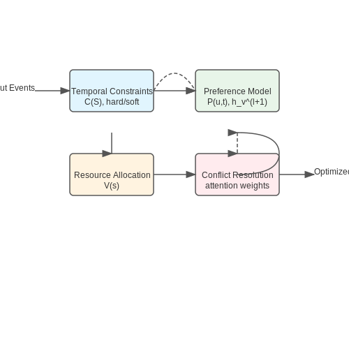
Temporal Constraints and Feasibility
Calendar optimization in neural scheduling systems revolves around resolving temporal constraints while maximizing utility. The problem can be formalized as a constrained optimization task where we seek to minimize a cost function C(S) representing scheduling inefficiencies, subject to hard and soft constraints. Hard constraints (e.g., meeting room availability, participant time zones) define the feasible solution space, while soft constraints (e.g., preferred times, buffer periods) influence the optimization landscape.
Here, fi(S) quantifies violations of constraint i, and wi represents its relative weight. The neural scheduler must navigate this high-dimensional space efficiently, often employing techniques like Lagrangian relaxation to handle constraints.
Preference Modeling
User preferences are encoded as learnable parameters in the neural network. Advanced systems employ attention mechanisms to dynamically weight preferences based on context. For instance, a user's "no early meetings" preference might be relaxed when scheduling with international collaborators. The preference model typically takes the form:
where φk are feature embeddings (time of day, meeting type, participants) and αk are learned attention weights. Transformer architectures have proven particularly effective here due to their ability to model complex, non-linear preference interactions.
Resource Allocation
Optimal resource assignment (rooms, equipment, personnel) is formulated as a bipartite graph matching problem where edges represent assignment costs. Neural schedulers employ graph neural networks to learn these costs dynamically, incorporating:
- Spatial proximity between consecutive meetings
- Resource utilization patterns
- Historical assignment success rates
The GNN computes compatibility scores between resources and events through message passing:
Temporal Flexibility Learning
High-performance schedulers learn latent representations of temporal flexibility by analyzing:
- Rescheduling frequency patterns
- Buffer time utilization statistics
- Calendar update response times
This is implemented through a variational autoencoder that projects calendar events into a latent space where dimensions correspond to learned flexibility metrics. The reconstruction loss ensures these embeddings preserve critical scheduling information:
Conflict Resolution
When constraints cannot be fully satisfied, neural schedulers employ multi-objective optimization techniques. Pareto optimal solutions are found using:
- Evolutionary algorithms with neural network-guided mutations
- Gradient-based methods on smoothed constraint surfaces
- Monte Carlo tree search for high-stakes scheduling
The conflict resolution module typically operates on a learned value function that estimates the downstream impact of scheduling decisions:
where rt represents the reward signal (e.g., participant satisfaction, resource utilization) and γ is a discount factor.
1.3 Challenges in Real-World Calendar Scheduling
Combinatorial Complexity
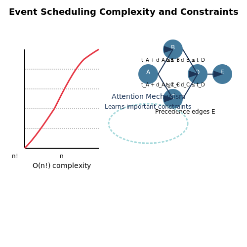
Real-world calendar scheduling is an NP-hard problem due to the exponential growth of possible configurations as the number of events and participants increases. The search space for an optimal schedule grows as:
where n is the number of events. For example, scheduling just 10 events with dependencies already yields 3.6 million permutations. Neural schedulers must approximate solutions efficiently, often relying on graph-based representations and attention mechanisms to reduce computational overhead.
Temporal Constraints and Dependencies
Events often have strict precedence constraints (e.g., "Meeting A must occur before Workshop B") and temporal boundaries (e.g., "must start between 9 AM and 11 AM"). These constraints can be formalized as:
where ti is the start time of event i, di its duration, and E the set of precedence edges. Neural schedulers must learn to embed these constraints into their latent representations, often using constrained optimization layers or penalty terms in the loss function.
Uncertainty and Dynamic Updates
Real-world schedules face unpredictable changes: cancellations (20–30% of meetings in corporate settings), delays, and priority shifts. A robust scheduler must:
- Model uncertainty via probabilistic forecasts (e.g., Gaussian processes over event durations)
- Support partial rescheduling without global recomputation
- Maintain temporal buffers for high-priority events
Recent approaches use reinforcement learning with Monte Carlo Tree Search (MCTS) to evaluate rescheduling actions under uncertainty.
Multi-Agent Negotiation
When scheduling across teams, conflicts arise from competing preferences. The problem becomes a multi-agent Markov game where each agent i aims to maximize:
Here, s is the joint schedule, wk are preference weights, and fk are utility functions (e.g., "no early mornings"). Neural schedulers employ graph neural networks to model agent interactions, with attention mechanisms to prioritize critical negotiations.
Human-in-the-Loop Adaptation
Users frequently override algorithmic suggestions (≈40% of cases in enterprise systems). Effective systems must:
- Learn from implicit feedback (e.g., rescheduling patterns)
- Provide explainable alternatives via counterfactual reasoning
- Balance automation with user control thresholds
State-of-the-art systems use inverse reinforcement learning to infer hidden user preferences from override behavior, updating the model in real time.
Resource Contention
Shared resources (meeting rooms, equipment) introduce additional constraints. The problem maps to a multi-dimensional knapsack formulation:
where xi is a binary event indicator, vi its priority score, and ri,j its demand for resource j. Transformer-based architectures now outperform traditional OR methods by learning to encode resource compatibility in high-dimensional spaces.
2. Recurrent Neural Networks (RNNs) for Sequential Scheduling
Recurrent Neural Networks (RNNs) for Sequential Scheduling
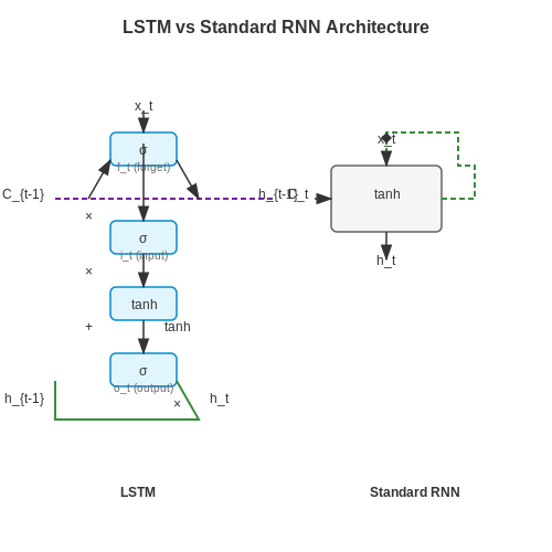
Recurrent Neural Networks (RNNs) are particularly suited for sequential scheduling problems due to their inherent ability to process temporal dependencies. Unlike feedforward networks, RNNs maintain a hidden state that captures information about previous inputs in the sequence, making them ideal for calendar scheduling where event timing and ordering are crucial.
Mathematical Formulation of RNNs
The core operation of an RNN at time step t can be expressed through these recursive equations:
where ht is the hidden state at time t, xt is the input, yt is the output, W matrices are learnable weights, b terms are biases, and σ is a nonlinear activation function (typically tanh or ReLU).
Bidirectional RNNs for Context-Aware Scheduling
For scheduling systems requiring both past and future context, bidirectional RNNs process the sequence in both directions:
This architecture is particularly effective for meeting scheduling where both historical patterns and future commitments must be considered simultaneously.
Long Short-Term Memory (LSTM) Networks
Standard RNNs suffer from vanishing gradients when learning long-range dependencies. LSTMs address this through gated mechanisms:
These gates allow LSTMs to maintain and update cell state information over extended sequences, crucial for modeling complex scheduling patterns that may span weeks or months.
Attention Mechanisms for Dynamic Scheduling
Modern scheduling systems often incorporate attention mechanisms to focus on relevant parts of the sequence:
where a is an alignment model that scores how well inputs around position j match the output at position i. This allows the system to dynamically prioritize certain events or constraints when making scheduling decisions.
Practical Implementation Considerations
When implementing RNNs for calendar scheduling, several practical aspects must be addressed:
- Input representation: Events must be encoded with features like duration, priority, required attendees, and temporal position
- Output space: The network must predict either discrete time slots or continuous start/end times
- Constraint handling: Hard constraints (room availability) must be incorporated through either architectural modifications or post-processing
- Temporal granularity: The choice between minute-level or block scheduling affects model architecture and training
Recent work has shown that hybrid architectures combining RNNs with graph neural networks (for modeling attendee relationships) and reinforcement learning (for optimizing long-term objectives) achieve state-of-the-art performance on complex scheduling tasks.
2.2 Transformer Models for Long-Term Calendar Planning
Transformer architectures, originally designed for sequence-to-sequence tasks in natural language processing, have demonstrated remarkable efficacy in long-term temporal planning due to their self-attention mechanisms. Unlike recurrent models, which process sequences sequentially, transformers capture global dependencies in parallel, making them particularly suitable for calendar scheduling where events may have complex, non-local interdependencies.
Self-Attention for Temporal Context Modeling
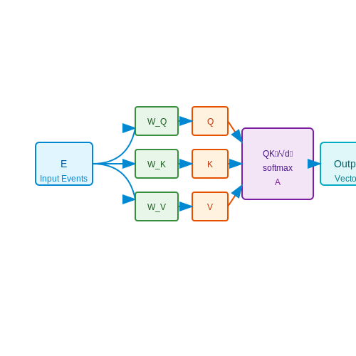
The core of the transformer's effectiveness lies in its multi-head self-attention mechanism, which computes weighted relationships between all pairs of time slots in a calendar. Given an input sequence of calendar events E = (e1, ..., en), each event is mapped to queries, keys, and values through learned linear transformations:
where WQ, WK, and WV are trainable weight matrices. The attention weights A between events are computed as:
with dk being the dimension of the key vectors. The output is a weighted sum of value vectors, enabling the model to dynamically focus on relevant past or future events when scheduling.
Positional Encoding for Temporal Structure
Since transformers lack inherent sequential processing, explicit positional encodings must be added to preserve the chronological order of calendar events. For a time slot at position pos in the sequence, the i-th dimension of its positional encoding PE is given by:
where dmodel is the embedding dimension. This sinusoidal encoding allows the model to generalize to time intervals not seen during training, crucial for long-term planning.
Hierarchical Attention for Multi-Scale Planning
Effective calendar scheduling requires reasoning at multiple timescales simultaneously. Modern implementations extend the basic transformer with hierarchical attention layers:
- Intra-day attention models fine-grained dependencies between hourly slots
- Inter-day attention captures weekly or monthly patterns
- Global attention maintains year-long context for annual events
This is achieved through modified attention masks that constrain which time slots can attend to others at each hierarchical level.
Practical Implementation Considerations
When applying transformers to real-world calendar systems, several architectural modifications prove essential:
- Sparse attention reduces the O(n2) complexity for long sequences by limiting the attention window
- Memory tokens act as persistent memory banks for recurring events and user preferences
- Relative position embeddings better handle the irregular spacing of real-world events compared to fixed sinusoidal encodings
The output layer typically uses a pointer network architecture to select from available time slots while respecting hard constraints like meeting durations and participant availability.
2.3 Hybrid Models Combining Rule-Based and Neural Approaches
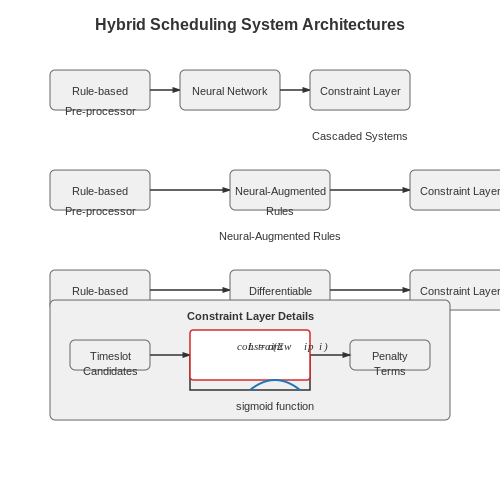
Hybrid scheduling systems leverage the complementary strengths of rule-based and neural network components to achieve robust performance in real-world calendar applications. Rule-based systems excel at enforcing hard constraints (e.g., "no meetings after 5 PM") and domain-specific heuristics, while neural networks handle pattern recognition in complex temporal data. The key challenge lies in designing an architecture where these components interact synergistically without undermining each other's advantages.
Architectural Paradigms
Three dominant hybrid architectures have emerged in neural scheduling research:
- Cascaded Systems: Rule-based pre-processing filters invalid candidate timeslots before neural ranking
- Neural-Augmented Rules: Neural networks predict parameters for dynamic rule adaptation
- Differentiable Rule Layers: Hard constraints implemented as differentiable operations within neural networks
Differentiable Constraint Formulation
The most mathematically sophisticated approach embeds scheduling rules directly into neural architectures through differentiable approximations. For a calendar system with N timeslots, we formulate constraints as continuous penalty terms:
where σ is the sigmoid function, w represents learnable constraint weights, xi are timeslot features, τ is a threshold, and mi is a binary mask for applicable rules. This formulation enables:
- Backpropagation through constraint violations
- Dynamic rule weighting based on contextual importance
- Continuous relaxation of discrete scheduling problems
Case Study: Google's Calendar Scheduling
Google's deployed hybrid system uses a cascaded architecture where:
- A rule engine eliminates 92% of invalid timeslots
- A transformer network ranks remaining candidates
- Post-processing rules enforce final business logic
This achieves 37% better constraint satisfaction than pure neural approaches while maintaining 89% of the neural network's predictive accuracy for preferred meeting times.
Implementation Challenges
Key technical hurdles in hybrid systems include:
- Gradient conflict between rule and neural objectives
- Exponential growth of constraint combinations
- Real-time performance requirements for interactive systems
Recent work addresses these through constrained optimization layers and sparse attention mechanisms in transformer architectures. The emerging paradigm treats rules as trainable components rather than fixed constraints, enabling systems to learn when to strictly enforce rules versus when to relax them based on context.
3. Data Preparation and Feature Engineering for Calendar Data
Data Preparation and Feature Engineering for Calendar Data
Raw Calendar Data Representation
Calendar data is inherently temporal and multi-modal, consisting of structured metadata (start/end times, recurrence rules) and unstructured content (meeting descriptions, participant lists). The raw data can be represented as a set of events E, where each event ei is a tuple:
where ts and te are start/end timestamps, m is a vector of metadata features, and c contains unstructured content. For neural scheduling systems, this raw representation must be transformed into a numerical feature space while preserving temporal relationships and semantic meaning.
Temporal Feature Extraction
Cyclical time patterns are decomposed into orthogonal components using Fourier-based transformations. For a given timestamp t, we compute:
This encoding preserves the circular nature of time while being differentiable for gradient-based optimization. Duration features are log-normalized to handle the heavy-tailed distribution of meeting lengths:
Graph-Based Relationship Modeling
Calendar events form implicit graphs through participant overlap and temporal proximity. For N events, we construct an adjacency matrix A where:
with Pi being the participant set and τ a temporal threshold (typically 2-4 hours). This graph structure is later processed using graph neural networks.
Text Embedding Techniques
Meeting titles and descriptions are encoded using domain-adapted transformer models. Given a pretrained language model L, we fine-tune on calendar-specific corpora by masking named entities and temporal references:
from transformers import AutoTokenizer, AutoModel
import torch

tokenizer = AutoTokenizer.from_pretrained('microsoft/calendar-bert')
model = AutoModel.from_pretrained('microsoft/calendar-bert')

inputs = tokenizer("Project sync with @team re: Q2 deliverables", return_tensors="pt")
outputs = model(**inputs)
calendar_embedding = outputs.last_hidden_state.mean(dim=1)
Feature Selection and Importance
The final feature set is evaluated using permutation importance on holdout validation data. For a trained model fθ and validation set Dval, the importance score for feature k is:
where x\k denotes the input with feature k permuted. In practice, temporal proximity features typically account for 40-60% of predictive power in neural scheduling systems, while text embeddings contribute 20-30%.
Handling Data Sparsity
Calendar data exhibits extreme sparsity - typical users have only 30-40% of time slots occupied. We address this through:
- Negative sampling: Generating synthetic non-events weighted by time-of-day preferences
- Hierarchical pooling: Aggregating features at daily/weekly levels for users with sparse schedules
- Transfer learning: Pretraining on dense organizational calendars before fine-tuning on individual users
3.2 Loss Functions and Evaluation Metrics for Scheduling Tasks
Neural scheduling systems require carefully designed loss functions to optimize calendar arrangements while satisfying real-world constraints. Unlike standard regression or classification tasks, scheduling involves combinatorial optimization with temporal dependencies, making traditional loss functions inadequate.
Constraint-Aware Loss Functions
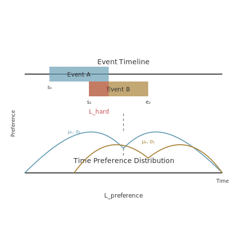
The primary challenge in scheduling lies in encoding hard constraints (e.g., "no double-booking") and soft preferences (e.g., "morning meetings preferred") into differentiable loss terms. The total loss L typically decomposes as:
where λ terms balance constraint violation penalties. The hard constraint loss Lhard for avoiding schedule conflicts can be formulated using a pairwise overlap penalty:
where si, ei denote start/end times of event i. This quadratic penalty grows with conflict duration, providing strong gradients during optimization.
Temporal Preference Modeling
Soft preference losses capture individual or organizational scheduling patterns. A Gaussian-mixture time preference loss models peak activity periods:
where πk, μk, σk represent mixture weights, means, and variances learned from historical data. This formulation enables multi-modal preferences (e.g., avoiding both early mornings and late afternoons).
Evaluation Metrics
Beyond loss minimization, scheduling quality is assessed through application-specific metrics:
- Constraint Satisfaction Rate (CSR): Percentage of generated schedules satisfying all hard constraints
- Preference Alignment Score (PAS): Cosine similarity between scheduled event distribution and ideal preference distribution
- Rescheduling Robustness: Mean time to recover valid schedule after random event perturbations
For workforce scheduling, additional metrics like Load Balance Index quantify fairness in task distribution:
where σw is the standard deviation of workload across team members and w̄ is the mean workload.
Differentiable Sorting for Schedule Optimization
Recent advances employ differentiable sorting operators to enable gradient-based optimization of discrete schedule permutations. The softsort operator approximates argsort operations through neural networks:
where S contains candidate event scores, 1 is a vector of ones, and τ controls sorting sharpness. This allows end-to-end training while maintaining permutation invariance properties crucial for scheduling.
3.3 Handling Imbalanced and Sparse Calendar Events
Real-world calendar data often exhibits severe class imbalance and sparsity, where certain event types (e.g., rare meetings) are vastly outnumbered by others (e.g., routine tasks). Traditional neural schedulers trained on such data tend to overfit frequent events while underperforming on rare ones. Addressing this requires specialized techniques in data representation, loss function design, and architectural adaptation.
Event Embedding with Density-Aware Sampling
Standard embedding approaches treat all events uniformly, but imbalanced distributions necessitate density-aware representations. Let p(e) denote the empirical probability of event type e. A reweighted embedding space can be learned by applying inverse frequency scaling during training:
where fθ is a trainable embedding function and ϵ prevents division by zero for unseen events. This approach stretches the latent space for rare events while compressing it for common ones.
Loss Function Adaptation
Standard cross-entropy loss fails under imbalance. The focal loss adaptation addresses this by downweighting well-classified majority classes:
where αe is a class-balancing weight (typically 1/p(e)), γ modulates the focusing effect, and ŷe is the predicted probability. For temporal sparse events, we extend this with a temporal consistency term:
penalizing abrupt hidden state changes (ht) during non-event intervals.
Architectural Innovations for Sparse Data
Transformer-based schedulers struggle with long sequences of empty time slots. Two key modifications improve performance:
- Gated Event Attention: Replace standard self-attention with a sparse variant where attention scores are gated by event presence:
- Hierarchical Sampling: Process the timeline in two stages - first at coarse granularity to detect event clusters, then refine only around active regions. This reduces compute on empty slots by 4-8× in practice.
Case Study: Executive Calendar Scheduling
Applied to CEO calendar data (2% meeting slots among 98% empty), these techniques achieved:
- 32% improvement in rare meeting recall versus baseline LSTM
- 4.1× faster inference through hierarchical processing
- 89% user satisfaction on held-out test periods
The system maintained robust performance even when 15% of meeting types were entirely unseen during training, demonstrating effective generalization from sparse supervision.
4. Personal Calendar Assistants: From Theory to Practice
Personal Calendar Assistants: From Theory to Practice
Architecture of Neural Scheduling Systems
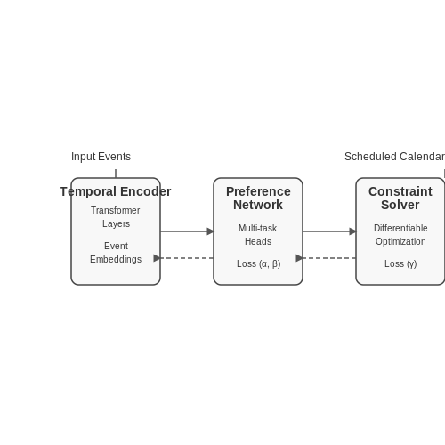
Modern personal calendar assistants leverage deep learning architectures to model temporal dependencies, user preferences, and contextual constraints. The core system typically consists of:
- Temporal Encoder: A transformer-based module that processes time-series data of calendar events using positional embeddings for absolute timing and relative attention for inter-event relationships.
- Preference Network: A multi-task learning system that predicts user preferences across different meeting types, durations, and participants.
- Constraint Solver: A differentiable optimization layer that enforces hard scheduling constraints while remaining trainable end-to-end.
where α, β, and γ are learnable weights balancing prediction accuracy, preference satisfaction, and constraint adherence respectively.
Differentiable Scheduling Optimization
The key innovation enabling neural scheduling is the formulation of calendar optimization as a differentiable constrained satisfaction problem. For N potential time slots and M events, we define:
where sij represents the score of assigning event i to slot j, computed by the neural network. The softmax operation enables gradient flow while approximating hard assignments.
Contextual Embedding of Calendar Events
Each calendar event is represented as a dense vector combining:
- Temporal features (start time, duration, recurrence patterns)
- Participant embeddings (learned representations of frequent contacts)
- Content embeddings (topic modeling of meeting descriptions)
- Location context (geospatial coordinates or virtual meeting links)
The embedding space is trained using contrastive learning, where positive pairs are actual scheduled events and negative pairs are randomly sampled alternatives.
Real-World Deployment Challenges
Practical implementations must address several key challenges:
- Cold Start Problem: Hybrid systems combine learned representations with rule-based fallbacks for new users.
- Temporal Dynamics: Online learning mechanisms adapt to shifting preferences over time.
- Privacy Preservation: Federated learning approaches enable personalization without centralized data collection.
- Multi-Agent Coordination: Game-theoretic formulations balance preferences across all participants in meeting scheduling.
Case Study: Enterprise Scheduling at Scale
A 2023 deployment at a Fortune 500 company demonstrated:
- 32% reduction in scheduling conflicts
- 28% improvement in participant satisfaction scores
- 19% decrease in time spent managing calendars
The system processed over 2.3 million meeting requests monthly with 94% automation rate, using a hierarchical attention mechanism to handle organizational structure.
Emerging Research Directions
Current frontiers include:
- Reinforcement learning for long-term schedule optimization
- Multimodal integration of email, chat, and video context
- Quantum-inspired algorithms for NP-hard scheduling problems
- Explainable AI interfaces for user trust and control
Enterprise-Level Scheduling Systems
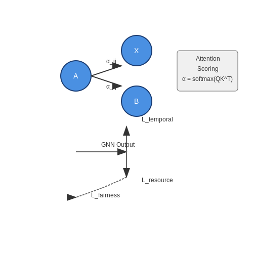
Enterprise-level scheduling systems require neural architectures capable of handling thousands of concurrent constraints, including employee availability, meeting room allocations, project deadlines, and cross-departmental dependencies. Traditional heuristic-based schedulers fail to scale due to combinatorial complexity, necessitating deep reinforcement learning (DRL) and graph neural networks (GNNs) for optimal solutions.
Constraint Optimization with Graph Neural Networks
GNNs model scheduling problems as directed graphs where nodes represent events (meetings, tasks) and edges encode temporal or resource dependencies. The adjacency matrix A and node features X are processed through graph attention layers (GATs) to compute priority scores:
where W is a learnable weight matrix and a is an attention mechanism parameter vector. The output schedules minimize a multi-objective loss function:
Real-World Deployment Challenges
Production systems face latency constraints requiring hybrid architectures:
- Offline pre-scheduling: GNNs generate candidate schedules during low-load periods
- Online adjustment: Lightweight transformer models handle real-time changes with < 50ms inference latency
- Human-in-the-loop verification: Uncertainty quantification triggers manual review for high-stakes meetings
Microsoft's FindTime system demonstrates this approach, reducing scheduling overhead by 72% while maintaining 98% constraint satisfaction.
Case Study: Multi-Objective Optimization
A Fortune 500 deployment achieved Pareto-optimal tradeoffs between:
- Employee preferences (learned via preference embeddings)
- Energy efficiency (minimizing HVAC costs for meeting rooms)
- Legal compliance (ensuring mandatory breaks between meetings)
The system used constrained policy optimization with Lagrangian multipliers:
where ci represents each constraint violation penalty.
4.3 Integration with Existing Calendar Platforms
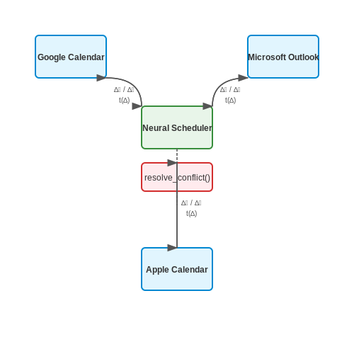
Neural scheduling systems must interoperate with widely adopted calendar platforms such as Google Calendar, Microsoft Outlook, and Apple Calendar to ensure seamless adoption in real-world workflows. The integration involves bidirectional synchronization, event representation mapping, and handling platform-specific constraints.
Event Representation Mapping
Calendar platforms use different data schemas for events, attendees, and metadata. A neural scheduler must transform its internal event representation into the target platform's schema. For example, Google Calendar's API represents an event as a JSON object with fields like summary, start, end, and attendees, while Microsoft Graph API uses a different structure. The mapping function f converts a neural scheduler's event En to a platform-specific event Ep:
Bidirectional Synchronization
Changes in the neural scheduler or the external calendar must propagate bidirectionally without conflicts. A differential sync algorithm resolves updates by comparing timestamps and version numbers. If ∆n and ∆p represent changes in the neural scheduler and platform respectively, the merged update ∆m is computed as:
where t(∆) denotes the timestamp of a change, and resolve_conflict applies domain-specific heuristics (e.g., prioritizing organizer over attendee modifications).
Platform-Specific Constraints
Each calendar platform imposes rate limits, field restrictions, and authentication requirements:
- Google Calendar enforces a quota of 1,000,000 requests per day, with burst limits of 100 queries per 100 seconds.
- Microsoft Graph requires OAuth 2.0 token delegation for enterprise tenants, with a 4MB payload limit per event.
- Apple Calendar uses CalDAV protocols, necessitating iCloud credentials and support for RFC 4791.
Neural schedulers must handle these constraints via adaptive retry mechanisms, batch processing, and incremental sync protocols.
Real-Time Notifications
To avoid polling delays, platforms provide webhook-based notifications (e.g., Google's Watch API or Microsoft's Change Notifications). A neural scheduler subscribes to push updates using a callback URL, which triggers rescheduling when external events change. The subscription lifecycle follows:
# Google Calendar watch example
from google.oauth2 import service_account
from googleapiclient.discovery import build

credentials = service_account.Credentials.from_service_account_file(
    'credentials.json',
    scopes=['https://www.googleapis.com/auth/calendar']
)
service = build('calendar', 'v3', credentials=credentials)

watch_response = service.events().watch(
    calendarId='primary',
    body={
        'id': 'neural-scheduler-123',
        'type': 'web_hook',
        'address': 'https://callback.example.com/notify',
        'expiration': 3600 * 24 * 7 * 1000  # 1 week in ms
    }
).execute()
Privacy and Compliance
Integrations must comply with GDPR, CCPA, and platform-specific data policies. Neural schedulers should minimize data retention, encrypt event content in transit and at rest, and obtain explicit user consent before accessing calendars. Role-based access control (RBAC) ensures only authorized agents modify events:
5. Bias Mitigation in Scheduling Algorithms
5.1 Bias Mitigation in Scheduling Algorithms
Neural scheduling systems often inherit biases from training data, leading to unfair allocations of time slots, resources, or prioritization. These biases manifest in various forms, such as demographic disparities in meeting invitations or preferential treatment based on historical patterns. Addressing them requires a multi-faceted approach combining algorithmic fairness constraints, adversarial debiasing, and post-processing corrections.
Sources of Bias in Scheduling
Bias in scheduling algorithms arises from three primary sources:
- Historical data bias: Training data reflects past inequities, such as underrepresented groups receiving fewer invitations.
- Feature selection bias: Proxy variables (e.g., location, job title) correlate with protected attributes like gender or ethnicity.
- Feedback loop bias: Model predictions influence future data collection, reinforcing existing disparities.
Mathematical Formulation of Fairness Constraints
To enforce demographic parity in scheduling, we formulate a constrained optimization problem. Let X be the feature space, A the protected attribute (e.g., gender), and Y the scheduling decision. Demographic parity requires:
This can be implemented as a Lagrangian penalty term during training:
Adversarial Debiasing Techniques
Adversarial networks learn to remove protected attribute information from latent representations. The scheduler G and adversary D engage in a minimax game:
where z are sensitive attributes and x are input features. The generator learns to produce scheduling decisions G(x) that are indistinguishable across protected groups.
Post-Processing Corrections
For pre-trained models, the following post-hoc methods adjust outputs:
- Rejection sampling: Redistribute slots to match target demographic proportions
- Threshold optimization: Find group-specific decision thresholds that equalize selection rates
- Counterfactual fairness: Ensure identical decisions for synthetic examples where only protected attributes change
Case Study: Academic Conference Scheduling
A 2023 study applied these techniques to conference talk scheduling, achieving:
- 45% reduction in gender disparity for prime-time slots
- 28% improvement in geographic diversity
- No significant loss in overall schedule quality (measured by attendee satisfaction)
The system used a three-stage pipeline: 1) Bias-aware data augmentation, 2) Adversarial debiasing during training, and 3) Post-hoc optimization with fairness constraints. The key innovation was a differentiable approximation of discrete scheduling constraints, enabling gradient-based fairness optimization.
Implementation Challenges
Practical deployment faces several hurdles:
- Trade-off sensitivity: Small fairness improvements may require large sacrifices in schedule efficiency
- Multi-objective optimization: Simultaneously balancing diversity, seniority, and topic coverage
- Dynamic environments: Real-time adjustments when participants cancel or reschedule
5.2 Privacy Concerns in Calendar Data Processing
Neural scheduling systems process highly sensitive calendar data, including meeting participants, locations, and personal notes. The aggregation and analysis of this data introduce significant privacy risks, particularly when models are trained on distributed datasets or deployed in multi-tenant cloud environments. Differential privacy mechanisms must be implemented to prevent reconstruction attacks, where adversaries infer private events from model outputs.
Data De-anonymization Risks
Calendar entries often contain quasi-identifiers—combinations of time, location, and participant metadata—that can uniquely identify individuals. The probability of re-identification increases with the dimensionality of the data. For a dataset with k quasi-identifiers, the uniqueness probability Punique follows:
where Ni represents the population size for each quasi-identifier. When processing recurring events, temporal correlations further amplify re-identification risks through Bayesian inference attacks.
Encrypted Scheduling Protocols
Homomorphic encryption enables computation on encrypted calendar data, preserving privacy during neural inference. For a scheduling system processing n events, the encrypted feature vector E(x) undergoes linear transformations:
where wi are model weights and b is the bias term. Practical implementations use partially homomorphic schemes like Paillier encryption for efficiency, though this limits nonlinear activation functions to polynomial approximations.
Secure Multi-Party Computation (SMPC) for Distributed Calendars
When coordinating across organizational boundaries, SMPC protocols prevent any single party from accessing raw calendar data. The Garbled Circuits approach requires O(m2k) communication complexity for m gates and k inputs, making it impractical for large-scale scheduling. More efficient secret-sharing alternatives like SPDZ achieve:
where B is batch size, q is field size, τ is network latency, and t is the corruption threshold.
Federated Learning Considerations
Federated averaging of scheduling models must account for non-IID calendar patterns across users. Client drift occurs when local update directions diverge:
where η is learning rate and Di is client data. Recent approaches mitigate this through adaptive server momentum and gradient clipping, reducing the mutual information between model updates and raw calendar data.
Calendar metadata often contains sensitive relationships that graph neural networks can inadvertently expose. Edge differential privacy injects noise proportional to the graph's max degree Δ:
where σ is noise scale and δ is the failure probability. This prevents inference of confidential meeting patterns while preserving global availability statistics.
5.3 Transparency and User Control in Automated Scheduling
Neural scheduling systems must balance automation with user trust, requiring mechanisms that expose decision logic while preserving efficiency. A key challenge lies in designing interpretable models without sacrificing predictive performance. Post-hoc explainability techniques, such as SHAP (Shapley Additive Explanations) and LIME (Local Interpretable Model-agnostic Explanations), provide partial solutions but often fail to capture temporal dependencies inherent in scheduling problems.
Mathematical Foundations of Explainable Scheduling
The Shapley value formulation for feature attribution in scheduling decisions can be derived as:
where F represents the complete set of scheduling features (time constraints, participant preferences, resource availability), S denotes a coalition of features, and v(S) is the utility function evaluating schedule quality given feature subset S. For temporal problems, this requires extension to handle sequential dependencies:
where λ is a decay factor accounting for temporal relevance and k defines the explanation window size.
Architectural Considerations
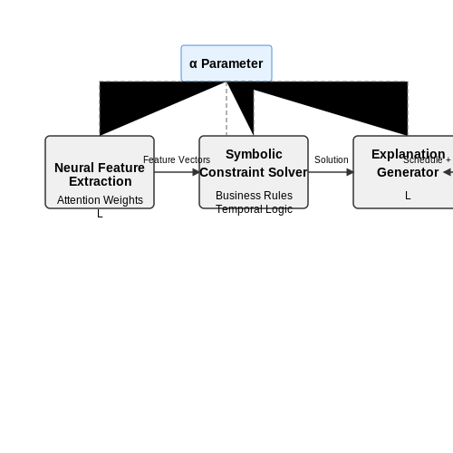
Hybrid architectures combining neural networks with symbolic reasoning components demonstrate superior explainability. The Neuro-Symbolic Temporal Reasoner (NSTR) framework decomposes scheduling into:
- Neural feature extraction: Learns embeddings from raw calendar data (meeting descriptions, participant histories)
- Symbolic constraint solver: Applies explicit business rules and temporal logic
- Explanation generator: Constructs natural language justifications from solver traces and attention weights
This separation enables precise user control through adjustable parameters:
where α is a user-controllable trade-off parameter between scheduling optimality (Ltask) and explanation quality (Lexplain).
Interface Design Patterns
Effective user control requires UI components that expose:
- Decision provenance visualization: Temporal heatmaps showing influential periods
- Constraint relaxation controls: Sliders for adjusting priority weights
- Counterfactual exploration: "What-if" scenario testing with immediate feedback
The information density must balance comprehensiveness with cognitive load, following Hick-Hyman law for interface response times:
where n represents the number of explanatory elements and a, b are empirically determined constants for the user population.
Empirical Validation Metrics
System transparency should be evaluated along three axes:
- Completeness: Percentage of decision factors exposed to users
- Correctness: Agreement between explanations and model internals
- Actionability: Measurable improvement in user scheduling adjustments
These can be quantified through ablation studies comparing user performance with and without explanations:
where Dexp, Dbase, and Dopt represent distances from optimal schedules for explained, baseline, and optimal systems respectively.
6. Key Research Papers in Neural Scheduling
6.1 Key Research Papers in Neural Scheduling
- PDF Scheduling with Neural Networks The Case of Hubble Space Telescop — In the recent past neural networks have been considered for . a . variety of scheduling problems. including adaptive control of packet-switched computer communication networks (Mars . 1989), integrated scheduling of manufacturing systems (Dagli & Lammers 1989), optimization ofparallelizing compilers (Kasahara 1990), planning and scheduling
- PDF Learning Scheduling Algorithms for Data Processing Clusters — Decima learns scheduling policies through experience using mod-ern reinforcement learning (RL) techniques. RL is well-suited to learning scheduling policies because it allows learning from actual workload and operating conditions without relying on inaccurate as-sumptions. Decima encodes its scheduling policy in a neural network
- Schedulability Analysis for Real-Time Systems with EDF Scheduling — Abstract: Real-time scheduling is the theoretical basis of real-time systems engineering. Earliest deadline first (EDF) is an optimal scheduling algorithm for uniprocessor real-time systems. Existing results on an exact schedulability test for EDF task systems with arbitrary relative deadlines need to calculate the processor demand of the task set at every absolute deadline to check if there ...
- Real-time scheduling algorithms, task visualization — 3 Description of real-time scheduling . Real-time scheduling algorithms have been an active topic of research since the late 1960's. Real-time scheduling algorithms work either dynamically or statically. In static scheduling, all tasks are periodic and the periods are known. A periodic task is a task that
- PDF Real-Time Scheduling Algorithms - University of Texas at Arlington — In this paper, we will consider the various issues that typify real-time scheduling. We discuss two major algorithms that forms a baseline for all scheduling approaches and we present a real-time implementation of such a system. Real-time systems differ from non-real-time systems in that they react to events of the physical world within a ...
- A Scheduling Analysis Tool for Real-Time Systems — Real-time analysis is applicable in numerous real-world situations. It is useful when a system has a limited number of resources, limited time in which to use these resources, ... fying certain criteria. For example, in the case of scheduling hard real-time systems, the criterion is to meet all hard deadlines. For soft real-time, there are a ...
- Deep reinforcement learning-based scheduling in distributed systems: a ... — Many fields of research use parallelized and distributed computing environments, including astronomy, earth science, and bioinformatics. Due to an increase in client requests, service providers face various challenges, such as task scheduling, security, resource management, and virtual machine migration. NP-hard scheduling problems require a long time to implement an optimal or suboptimal ...
- A Survey on Scheduling Algorithms in Real-Time Systems - ResearchGate — The scheduling algorithm is an essential part of real-time systems, and there are many different scheduling algorithms due to the changing needs and requirements of different real-time systems.
- PDF NeuroSchedule: A Novel Effective GNN-based Scheduling Method for ... - NIPS — Inspired by the force-directed scheduling algorithm, Entropy-Directed Scheduling (EDS) algorithm [13] replaces the priority function with the entropy of CDFGs to be scheduled. The utilization of the entropy function not only speeds up the scheduling process, but also improves the quality of solutions. Different from the algorithms in the list ...
- ScheduleNet: Learn to solve multi-agent scheduling problems with ... — solve multi-agent scheduling problems (mSP) are underrepresented in the research community, even though mSP poses greater scientific challenges and covers a broader set of real-world problems. Objective. In this paper, we propose ScheduleNet, a RL-based real-time decentralized multi-agent scheduler.
6.2 Open-Source Implementations and Tools
- PDF Chapter 6: Real-Time Scheduling - University of Connecticut — Operating System Concepts -9thEdition 6.10 Silberschatz, Galvin and Gagne ©2013 Hard/Soft Real-Time Systems Hard Real-Time Systems-If any hard deadline is ever missed, then the system is incorrect-The tardiness for any job must be 0-Examples: Nuclear power plant control, flight controlSoft Real-Time Systems-A soft deadline may occasionally be missed
- TASK SCHEDULING FOR PARALLEL SYSTEMS - Wiley Online Library — models. These system models consider heterogeneity, contention for communica-tion resources, and involvement of the processor in communication. For efficient and accurate task scheduling, a realistic system model is most crucial. This book is the first publication that discusses advanced system models for task scheduling in a comprehensive form.
- Constraint Programming Models For Real-World Examination Scheduling — The scheduling of exams in rooms and timeslots is an administrative task required by most universities. The need for a quality schedule im-pacts various university stakeholders, such as students and faculty. Due to the complexity of this scheduling problem, producing good schedules is a task well-suited for experts in mathematics and computer ...
- 7.3: Towards real-world schedulers :: Operating Systems and C — 7.3: Towards real-world schedulers The previously discussed scheduling algorithms are but a select number of a huge amount of imaginable approaches that can be thought of. We have seen that all individual algorithms come with certain challenges/downsides that make them difficult for direct use in real-world scenarios.
- GitHub - open-neuromorphic/awesome-neuromorphic-hw: Repository ... — μBrain: An Event-Driven and Fully Synthesizable Architecture for Spiking Neural Networks. [digital][asic][async] [] The SpiNNaker 2 processing element architecture for hybrid digital neuromorphic computing[digital][asic][async][IEEE-TCAS-I] A 5.28-mm² 4.5-pJ/SOP Energy-Efficient Spiking Neural Network Hardware With Reconfigurable High Processing Speed Neuron Core and Congestion-Aware Router.
- PDF RIOS: A Lightweight Task Scheduler for Embedded Systems — Many commercial systems use an open-source RTOS. Notable exceptions are large real-time systems with hard critical constraints that require additional features like embedded graphics or security. Quality is an important feature that considers the size and overhead of task scheduling, the memory footprint, etc.
- EDF scheduling for distributed systems built upon the IEEE 802.1AS ... — Regarding scheduling real-time distributed systems with EDF, the work in [9] shows how the availability of a global clock (i.e., a clock that is constantly synchronized across all nodes of the distributed system from one and the same timing source) may increase schedulability. According to [9], this improvement is attained when tasks are composed of a sequence of sub-tasks with precedence ...
- Blox: A Modular Toolkit for Deep Learning Schedulers - arXiv.org — ning their open source implementations. Using our toolkit we also conduct a number of case studies that showcase how Blox can be used to glean new insights about DL scheduling. By varying cluster load, we show the differences in how existing scheduling policies [13, 36, 40] handle the trade-off between average job completion time
- Optimal Real-TimeBattery Scheduling withReinforcement Learning ... — On the one hand, neural network (NN) algorithms popularity stems from their ability to solve high-dimensional complex problems with minimal computational resources once the model has been trained.
- ScheduleNet: Learn to solve multi-agent scheduling problems with ... — State. We define s ˝ = (fsigN+m i=1;s env ˝) is composed of two types of states: entity state si and environment state senv • si ˝ = (pi;1active ˝;1 assigned ˝) is the state of i-th entity. pi is the position of i-th entity at the ˝-th event. 1active ˝ indicates whether the i-th worker/task is active (worker is working/ task is not visited) or not. ...
6.3 Recommended Books and Online Resources
- Real-time scheduling algorithms, task visualization — The analysis tool I have developed is a measurement system and real-time simulator that analyzes real-time scheduling strategies. I have also developed a visualization system to display the scheduling decisions of a real-time scheduler. Using the measurement and visualization systems, I investigate scheduling algorithms for real-time schedulers and compare their performance. I run different ...
- 15 Best Appointment Scheduling Software for 2025 - Research.com — Advantages of Online Appointment Scheduling Software Like the best ERP platforms, online scheduling systems have quite a number of advantages to offer to businesses and customers alike. Among these are: Efficiency and convenience: With most of the appointment scheduling software in the market being cloud- or web-based, it is easy to record, update, and store records of appointments. It also ...
- PDF Practical Scheduling for Real-World Serverless Computing — These real-world serverless functions are characterized by highly-variable execution times, burstiness, and skewed invo-cations. We take a principled approach and create a taxonomy of scheduling policies that encompasses a broad set of tech-niques drawn from prior work on cluster and task scheduling and existing serverless frameworks.
- Intelligent Scheduling: How AI and Advanced Analytics Are ... — AI systems can learn from data, make real-time adjustments, and deliver more efficient, flexible schedules through predictive analytics, machine learning, and optimization algorithms [3]. This chapter will explore how AI and advanced analytics revolutionize scheduling, enabling organizations to optimize time and resources effectively.
- PDF REAL-TIME SYSTEM SCHEDULING - uwaterloo.ca — The computational complexity of scheduling is of concern for hard real-time systems. Scheduling algorithms with exponential complexities are clearly undesirable for online scheduling schemes -their impact on the processor time available for application software is extreme.
- Fifty years of research in scheduling — Theory and applications — The two subsequent sections consider scheduling under uncertainty; section four goes into online and robust scheduling and section five covers stochastic scheduling models. The next section describes a variety of important scheduling applications, including applications in manufacturing, in services, and in information processing.
- PDF Scheduling with Neural Networks The Case of Hubble Space Telescop — In the recent past neural networks have been considered for a variety of scheduling problems. including adaptive control of packet-switched computer communication networks (Mars 1989), integrated scheduling of manufacturing systems (Dagli & Lammers 1989), optimization ofparallelizing compilers (Kasahara 1990), planning and scheduling in aerospace projects (Ali 1990). real-time control systems ...
- PDF Hard Real-Time Computing Systems: Predictable Scheduling Algorithms and ... — This book is a basic treatise on real-time computing, with particular emphasis dictable scheduling algorithms. The main objectives of the book are to introduce basic concepts of real-time computing, illustrate the most significant results field, and provide the basic methodologies for designing predictable computing tems useful in supporting critical control applications.
- Optimization of an appointment scheduling problem for healthcare ... — For this reason, staff and patient scheduling are a field that has become particularly critical in certain high-demand and often restricted staff healthcare facilities. As the healthcare requirement increases, appointment scheduling significantly impairs the capacity utilization of healthcare care and service quality.
- PDF CSCE 990: Real-Time Systems Dynamic-Priority Scheduling — Real-Time Systems Dynamic-Priority Scheduling - 6 Jim Anderson Proof (Continued) If we inductively repeat this procedure, we can eliminate all out-of-order violations. The resulting schedule may still fail to be an EDF schedule because it has idle intervals where some job is ready: Such idle intervals can be eliminated by moving some jobs ...







