Sparse Mixture-of-Experts Routing
1. Key Concepts and Architecture
1.1 Key Concepts and Architecture
Core Idea of Sparse Mixture-of-Experts
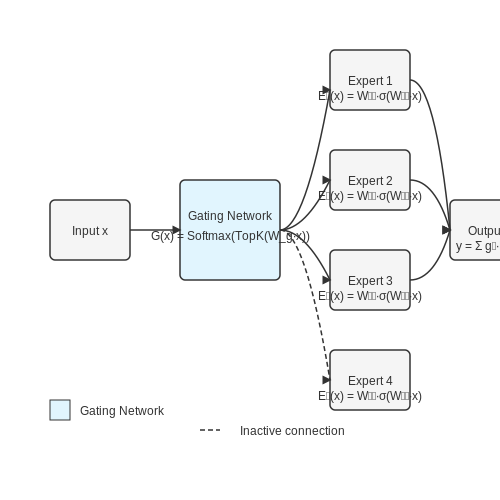
The sparse Mixture-of-Experts (MoE) model is a neural network architecture that dynamically routes input data to specialized subnetworks (experts) rather than processing all inputs through every parameter. Unlike dense models, MoE achieves computational efficiency by activating only a subset of experts per input. The routing mechanism is governed by a trainable gating network that produces sparse combinations, enabling the model to scale to thousands of experts while maintaining tractable computation.
where G(x) is a sparse gating function selecting k out of n experts Ei, and y is the weighted output. The sparsity constraint ensures G(x) has only k non-zero entries, typically with k ≪ n (e.g., k=2 for models like Switch Transformers).
Gating Mechanisms
The gating network computes expert selection probabilities via a softmax over learned weights. For input x, the gating logits Wgx are transformed into probabilities:
TopK retains only the k highest values, and ε is optional noise for load balancing (e.g., as in Noisy Top-K Gating). The sparsity introduces challenges in gradient estimation, often addressed via straight-through estimators or reinforcement learning techniques.
Expert Architecture
Each expert Ei is typically a feedforward network (FFN) with independent parameters. For a Transformer-based MoE layer, experts replace the standard FFN sublayer, with identical input/output dimensions to ensure compatibility. The experts operate in parallel, and their outputs are aggregated by the gating weights:
Load Balancing
A critical challenge is ensuring equal utilization of experts. Imbalanced routing can lead to underused or overloaded experts, degrading performance. Common solutions include:
- Importance loss: Penalizes deviations from uniform expert usage.
- Capacity factor: Limits the number of tokens per expert.
- Noise-based exploration: Adds stochasticity to gating decisions.
Scalability and Efficiency
Sparse MoE models achieve sublinear compute growth with respect to parameter count. For n experts and k-active selection, the compute cost scales as O(d2k + dn) per token (vs. O(d2n) for dense models), where d is the hidden dimension. This enables models like Google's Switch Transformer (1.6 trillion parameters) to remain feasible for training and inference.
Historical Context and Evolution
The concept of Mixture-of-Experts (MoE) originated in the early 1990s as a modular neural network architecture designed to improve computational efficiency and specialization. The foundational work by Jacobs et al. (1991) introduced the idea of partitioning a learning system into multiple expert networks, each responsible for a subset of the input space, with a gating mechanism dynamically routing inputs to the most relevant experts. This approach aimed to mitigate the limitations of monolithic neural networks, such as poor scalability and inefficient resource utilization.
Early Developments and Theoretical Foundations
Initial MoE models relied on soft, differentiable gating mechanisms, typically implemented via a trainable softmax function. The gating weights G(x) for an input x were computed as:
where W_g and b_g are learnable parameters. While effective, these models faced challenges in scaling to large numbers of experts due to the quadratic growth in computational complexity. The introduction of sparsity constraints in the late 2000s, particularly through top-k routing, marked a pivotal shift. Instead of activating all experts, only the top k experts with the highest gating scores were selected, reducing computation to O(k) per input:
Modern Advances and Large-Scale Applications
The resurgence of MoE models in the 2010s was driven by their integration into large-scale language models. Google's Switch Transformer (2021) demonstrated that sparse MoE routing could achieve state-of-the-art performance while maintaining computational efficiency. Key innovations included:
- Dynamic Routing: Input-dependent expert selection, enabling adaptive computation.
- Load Balancing: Techniques like auxiliary loss terms to prevent expert underutilization.
- Hardware-Aware Design: Optimizations for distributed training across GPUs/TPUs.
Recent work has further refined routing algorithms, incorporating reinforcement learning (Shazeer et al., 2023) and differentiable sparsity mechanisms (Lepikhin et al., 2022). These advances have solidified sparse MoE as a cornerstone of efficient large-scale deep learning.
1.3 Advantages Over Dense Models
Sparse Mixture-of-Experts (MoE) models fundamentally differ from dense architectures by activating only a subset of parameters per input, enabling superior computational efficiency without sacrificing model capacity. The key advantages stem from dynamic routing mechanisms that selectively engage expert networks, in contrast to dense models that uniformly process all inputs through every layer.
Computational Efficiency and Scalability
The computational cost of a dense model scales linearly with its parameter count, as every input must propagate through all layers. In contrast, sparse MoE models achieve sub-linear compute scaling by activating only k out of N experts per input. The effective computation follows:
where Crouter represents the overhead from gating operations. For large N (e.g., 2048 experts) and small k (e.g., 2-4), this reduces FLOPs by orders of magnitude while maintaining model capacity. Empirical studies show that MoE models can achieve comparable performance to dense models with 4-10x fewer FLOPs during inference.
Specialization and Multi-Task Learning
Expert networks naturally specialize in distinct input domains without explicit supervision. The routing mechanism clusters semantically similar inputs to the same experts, as demonstrated by the emergence of:
- Linguistic feature specialists (e.g., syntax vs. semantics)
- Domain-specific experts (e.g., scientific vs. conversational text)
- Task-oriented partitions in multi-task learning scenarios
This contrasts with dense models that must encode all features in shared parameters, often leading to interference between unrelated tasks. The sparse gradient updates in MoEs further mitigate catastrophic forgetting during continual learning.
Memory Efficiency and Distributed Training
While total parameter counts may be larger, sparse MoEs enable more efficient memory utilization through:
- Parameter offloading: Inactive experts can be paged to CPU or secondary storage
- Distributed parallelism: Experts naturally map to different devices with minimal communication
- Dynamic batch sizing: Variable compute per sample enables better hardware utilization
The memory access pattern becomes:
compared to dense models requiring full parameter loading (Mdense). This allows training models with trillions of parameters that would be infeasible with dense architectures.
Robustness and Noise Immunity
Sparse activation confers inherent robustness benefits:
- Fault tolerance: The failure of individual experts affects only their specialized subdomains
- Noise filtering: Routing networks learn to avoid corrupted or out-of-distribution inputs
- Adaptive computation: Difficult inputs can engage more experts dynamically
This contrasts with dense models where any parameter corruption affects all predictions uniformly. The sparse gradient flow also makes MoEs less susceptible to adversarial perturbations that require coordinated changes across many parameters.
Practical Deployment Advantages
In production systems, sparse MoEs enable:
- Dynamic load balancing by adjusting k based on latency requirements
- Incremental updates by retraining only relevant experts
- Hardware efficiency through expert-specific quantization and pruning
The routing mechanism effectively creates a content-addressable memory system, where similar inputs consistently activate the same expert subsets. This property enables novel caching strategies and reduces redundant computation for recurring input patterns.
2. Principles of Sparse Gating
Principles of Sparse Gating
Sparse gating is a fundamental mechanism in mixture-of-experts (MoE) models that dynamically routes input tokens to a small subset of expert networks. Unlike dense routing, which activates all experts for every input, sparse gating enforces sparsity by selecting only the top-k experts, reducing computational cost while maintaining model capacity. The gating function G(x) computes expert selection probabilities for an input x, typically using a softmax over learned gate weights.
Mathematical Formulation
The sparse gating function G(x) is defined as:
where Wg is a trainable weight matrix, ε is optional noise (e.g., for load balancing), and Topk retains only the k highest values. The softmax is applied to the sparsified logits, ensuring the output is a valid probability distribution. For a model with N experts, this reduces computation from O(N) to O(k) per token.
Noisy Top-k Gating
To encourage balanced expert utilization, a common variant adds tunable Gaussian noise before applying Topk:
The noise standard deviation σ is often annealed during training. This stochasticity prevents the "rich-get-richer" phenomenon where a few experts dominate the routing decisions.
Differentiability and Gradient Flow
Though Topk is non-differentiable, the gating mechanism remains trainable via straight-through estimation (STE). During the backward pass, gradients are propagated as if the selection were continuous. The expert weights Wg are updated using these proxy gradients, enabling end-to-end training.
Practical Considerations
- Expert Capacity: Each expert processes a variable number of tokens. Fixed-capacity buffers prevent memory overflow but may drop tokens when oversubscribed.
- Load Balancing: Auxiliary losses penalize uneven routing distributions to maintain expert utilization.
- Hardware Efficiency: Sparse routing enables conditional computation, where only activated experts execute, reducing FLOPs on specialized accelerators like TPUs.
Top-k Routing Strategies
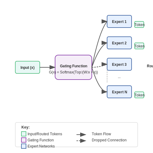
Top-k routing is a widely adopted strategy in sparse Mixture-of-Experts (MoE) models to balance computational efficiency with model performance. Unlike dense models where all parameters are active for every input, MoE models selectively activate only a subset of experts per input. The top-k mechanism achieves this by routing each input token to the k most relevant experts based on a learned gating function.
Gating Mechanism and Routing Probability
The gating function G(x) computes a score for each expert, typically using a softmax over a learned weight matrix. For an input x, the gating scores are computed as:
where Wg is the gating weight matrix and ϵ is optional noise (e.g., Gaussian or Gumbel noise) for exploration during training. The top-k experts are selected based on the highest scores in G(x).
Mathematical Formulation
Given the gating scores G(x) = [g1, g2, ..., gN] for N experts, the top-k routing can be formalized as:
The selected experts process the input, and their outputs are combined via a weighted sum:
where Eij(x) is the output of the j-th selected expert.
Practical Considerations
Top-k routing introduces several trade-offs:
- Computational Efficiency: Only k experts are active per input, reducing FLOPs compared to dense models.
- Expert Utilization: Without additional constraints, some experts may be underutilized (e.g., "expert imbalance"). Techniques like load balancing or auxiliary losses address this.
- Gradient Estimation: The top-k operation is non-differentiable. Straight-through estimators or Gumbel-softmax tricks are often used during training.
Variants and Extensions
Several variants improve upon basic top-k routing:
- Noisy Top-k: Adds stochasticity by sampling k experts proportionally to their scores, improving exploration.
- Top-k with Capacity: Limits the number of tokens per expert to avoid overload, critical for distributed training.
- Adaptive k: Dynamically adjusts k per input based on gating confidence or task complexity.
Case Study: Switch Transformers
Google's Switch Transformer uses top-1 routing (k=1) for extreme sparsity, achieving faster inference while maintaining model quality. The gating function is trained with auxiliary losses to ensure balanced expert usage.
Dynamic vs. Static Routing
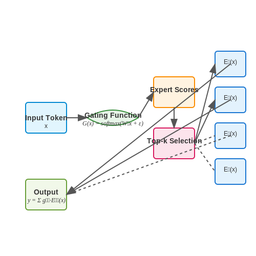
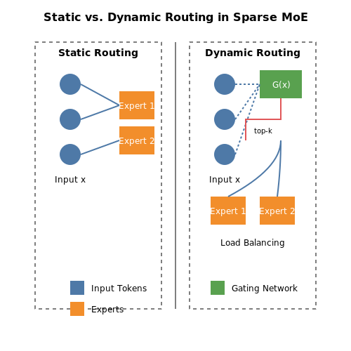
In sparse Mixture-of-Experts (MoE) models, routing mechanisms determine how input tokens are assigned to expert networks. The choice between dynamic and static routing fundamentally impacts model performance, computational efficiency, and adaptability to varying input distributions.
Static Routing
Static routing predefines expert assignments based on fixed rules or heuristics, independent of input data. A common approach partitions the input space uniformly or via clustering during training. For example, if experts are indexed by k and inputs lie in d-dimensional space, static routing might assign input x to expert k via:
where w is a learned projection vector and σ is a sigmoid function. This method is computationally efficient but lacks adaptability, as expert assignments remain rigid during inference regardless of input characteristics.
Dynamic Routing
Dynamic routing adjusts expert assignments based on input features, typically using a trainable gating network. The gating function G(x) computes a probability distribution over experts, often via a softmax over learned scores:
where W_g and b_g are gating parameters. To enforce sparsity, top-k routing selects only the k experts with highest probabilities, reducing computation by activating a subset of the model. The routing loss L_r may include auxiliary terms like load balancing to ensure equitable expert utilization:
where CV is the coefficient of variation of expert assignments f_k, and λ controls the balancing strength.
Trade-offs and Practical Considerations
Static routing excels in low-latency applications where deterministic behavior is critical, such as embedded systems. Dynamic routing, while more computationally intensive, adapts to heterogeneous data—e.g., in multilingual NLP tasks where input language distribution varies. Recent hybrid approaches combine static partitioning with dynamic fine-tuning, such as BASE layers, which use static blocks but dynamically route within them.
Empirical studies show dynamic routing improves model quality by 10-30% on perplexity metrics in language modeling, at the cost of 15-20% higher FLOPs per token. Techniques like expert caching or gradient accumulation mitigate this overhead by reusing expert computations across tokens with similar routing paths.
3. Balancing Expert Utilization
Balancing Expert Utilization
In sparse Mixture-of-Experts (MoE) models, routing mechanisms must ensure balanced workload distribution across experts to prevent underutilization or overloading. The primary challenge lies in maintaining high model capacity while avoiding scenarios where a small subset of experts dominates computation. This section examines key techniques for achieving balanced expert utilization.
Load Balancing Loss
The most common approach introduces an auxiliary loss term during training to penalize imbalanced routing. For a batch of N inputs, let f_i be the fraction of inputs routed to expert i, and p_i be the desired target distribution (typically uniform). The load balancing loss L_balance is computed as:
where λ controls the trade-off between task performance and balance. This KL-divergence formulation pushes the router to distribute workload according to p_i while preserving the model's ability to make input-dependent routing decisions.
Expert Capacity Constraints
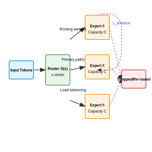
Practical implementations often enforce hard constraints on expert capacity to prevent overload. For a system with E experts processing N tokens, each expert is allocated a fixed capacity C = k·N/E, where k > 1 is a buffer factor. Tokens exceeding an expert's capacity are either:
- Dropped (reducing computation but potentially losing information)
- Re-routed to the next-best expert (maintaining model capacity at higher computational cost)
- Handled via auxiliary buffers (increasing memory overhead)
Adaptive Routing Strategies
Advanced routing mechanisms dynamically adjust expert selection based on real-time load conditions. The gating function G(x) can be modified to incorporate expert utilization feedback:
where u is a vector of current expert utilization rates and α controls the strength of the balancing effect. This approach creates a negative feedback loop - as an expert's utilization increases, its selection probability decreases.
Importance Weighting
Some implementations differentiate tokens by importance when enforcing balance. The router assigns each token an importance score I(x), typically derived from the gating weights themselves:
High-importance tokens receive priority during expert assignment, while low-importance tokens may be re-routed or dropped when capacity constraints are encountered. This preserves model performance on critical inputs while maintaining overall balance.
Empirical Considerations
In practice, the optimal balancing strategy depends on the specific architecture and task:
- Models with many experts (>64) typically require stronger balancing constraints
- Tasks with high input variability benefit from adaptive routing
- Distributed systems must consider network overhead of expert placement
3.2 Gradient Challenges and Solutions
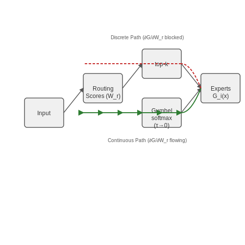
Sparse Mixture-of-Experts (MoE) models rely on discrete routing decisions to select subsets of experts for each input. While this sparsity enables computational efficiency, it introduces significant gradient estimation challenges during training. The primary issue stems from the non-differentiability of the expert selection process, which prevents standard backpropagation from flowing through the routing mechanism.
Gradient Estimation in Discrete Routing
The routing function in MoE models typically involves a top-k operation over expert scores, where only the highest-scoring experts are activated. Mathematically, for input x, the routing weights G(x) can be expressed as:
where Wr represents the routing weights and top-k selects only the k largest values. The discontinuous nature of top-k prevents direct gradient computation with respect to Wr.
Straight-Through Estimator (STE)
A common solution is the straight-through estimator, which approximates gradients by treating the top-k operation as the identity function during backpropagation. While simple, STE introduces bias because the forward and backward passes are inconsistent:
This approximation works reasonably well in practice but can lead to unstable training when expert selection is highly sensitive to small changes in routing scores.
Gumbel-Softmax Relaxation
For more stable gradient estimation, the Gumbel-softmax trick provides a continuous relaxation of the discrete routing decision. By adding Gumbel noise and using a temperature-controlled softmax, the routing becomes differentiable:
where gi are i.i.d. Gumbel samples and τ is a temperature parameter. As τ → 0, this approaches the discrete top-k selection while remaining differentiable for τ > 0.
Importance Sampling for Sparse Gradients
An alternative approach uses importance sampling to estimate gradients without requiring full differentiability. By treating expert selection as a stochastic process, gradients can be estimated via:
where S is the number of samples and p(s|x) is the routing probability distribution. This method works particularly well when combined with variance reduction techniques like REINFORCE with baseline.
Load Balancing for Gradient Stability
Beyond gradient estimation, MoE models face challenges with expert load imbalance, where gradients can become unstable if certain experts are over- or under-utilized. Common solutions include:
- Auxiliary loss terms that penalize unbalanced routing distributions
- Expert capacity constraints that enforce hard limits on expert usage
- Random routing with probability proportional to expert capacity
These techniques help maintain stable gradient flow by ensuring all experts receive sufficient training signals throughout the optimization process.
Scalability in Large-Scale Deployments
Scaling sparse Mixture-of-Experts (MoE) models to large deployments introduces unique computational and routing challenges. The primary bottleneck lies in the dynamic expert selection mechanism, where the gating network must efficiently route tokens to a subset of experts while minimizing cross-device communication overhead.
Efficient Distributed Routing
In distributed settings, experts are partitioned across multiple devices, requiring careful coordination to avoid excessive cross-device communication. The routing function must satisfy two constraints:
- Load balancing: Ensure no single expert is overwhelmed with tokens.
- Locality awareness: Prefer routing tokens to experts on the same device when possible.
The modified gating function for distributed MoE can be expressed as:
where masklocal(x) adds a bias term favoring local experts, and ε controls the trade-off between load balancing and locality.
Hierarchical Routing Strategies
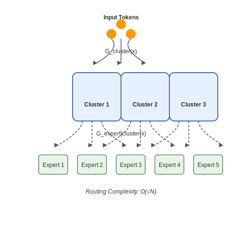
For deployments spanning thousands of experts, hierarchical routing reduces coordination overhead:
- First-level routing assigns tokens to device clusters
- Second-level routing selects specific experts within each cluster
This approach reduces the routing decision space from O(N) to O(√N) for N experts. The hierarchical gating function decomposes as:
Communication-Efficient Implementations
Modern MoE systems use several optimizations to reduce communication:
- Expert caching: Frequently-used experts are replicated across devices
- Batched routing: Group tokens into larger batches before routing decisions
- Gradient accumulation: Aggregate gradients across multiple steps before expert updates
The communication cost C for a distributed MoE layer scales as:
where T is the number of tokens, B the batch size, E the number of experts, and d the hidden dimension.
Hardware-Aware Routing
Advanced deployments incorporate hardware metrics into routing decisions:
- Device memory capacity
- Network bandwidth between devices
- Current GPU utilization
The hardware-aware routing score combines these factors:
where the coefficients are learned during training through backpropagation of the system performance metrics.
4. Natural Language Processing (NLP)
Sparse Mixture-of-Experts Routing in Natural Language Processing
Architecture and Routing Mechanisms
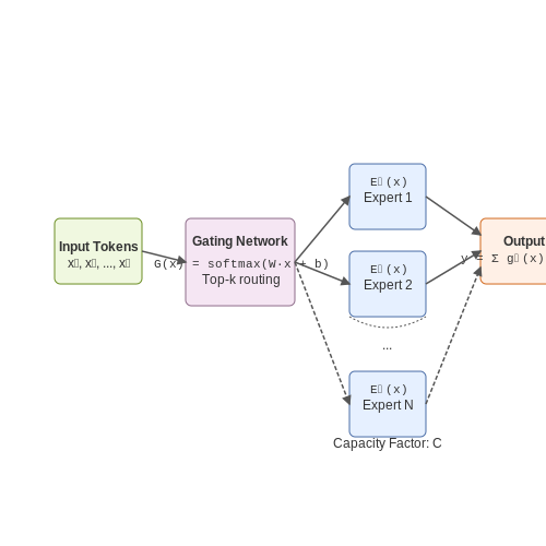
Sparse Mixture-of-Experts (MoE) models in NLP dynamically route input tokens to specialized subnetworks (experts) through a gating mechanism. Given an input token x, the gating network computes probabilities for expert selection:
where Wg and bg are trainable parameters. Only the top-k experts with highest probabilities are activated, enforcing sparsity. The output y combines expert outputs Ei(x) through weighted summation:
Capacity Factor and Load Balancing
Two critical constraints govern expert utilization:
- Capacity factor (C): Multiplier defining maximum tokens per expert (e.g., C=1.25 reserves 25% buffer capacity)
- Load balancing loss: Penalizes uneven routing distributions. For m experts, the auxiliary loss term is:
where CV is the coefficient of variation and λ scales the penalty (typically 0.01-0.1). This prevents expert underutilization ("starving experts") common in naive top-k routing.
Switch Transformer Case Study
Google's Switch Transformer scales MoE to trillion-parameter models by:
- Using k=1 routing (single expert per token) with C=1.0-2.0
- Implementing expert parallelism across TPU pods
- Adding dropout (rate=0.1) and layer normalization within experts
The gating network employs a temperature-scaled softmax for sharper routing decisions:
where temperature T anneals from 1.0 → 0.01 during training.
Token-Level vs. Sentence-Level Routing
Recent variants explore hierarchical routing:
- Token-level: Classic approach (e.g., Switch Transformer)
- Sentence-level: Routes entire sequences to experts (reduces communication overhead)
- Hybrid: First routes sentences, then tokens within selected experts
Sentence-level routing uses mean-pooled representations for gate computation:
Gradient Challenges and Solutions
Straight-through estimation (STE) bypasses non-differentiable top-k operations during backpropagation. For expert j and token x, the gradient approximation is:
where 𝕀 is an indicator function. Advanced variants like soft MoE replace hard routing with differentiable attention over experts.
4.2 Computer Vision and Multimodal Tasks
Sparse Mixture-of-Experts (MoE) models have demonstrated significant success in scaling neural networks for computer vision and multimodal learning. Unlike dense architectures, MoE models dynamically activate only a subset of experts per input, enabling efficient computation while maintaining high capacity. In vision tasks, this approach is particularly advantageous due to the high-dimensional, spatially structured nature of the data.
Routing Mechanisms in Vision Transformers
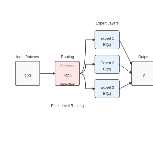
Modern vision transformers (ViTs) integrate MoE layers by replacing dense feed-forward networks with expert layers. The routing function g(x) determines expert selection for an input patch x. For a ViT with N experts, the output y of an MoE layer is computed as:
where gi(x) is the routing weight for expert Ei, typically computed via a softmax over learned scores. Sparse gating enforces top-k selection, where only k experts with highest weights are activated. The gating function can be formulated as:
Multimodal Expert Specialization
In multimodal settings (e.g., vision-language tasks), experts can specialize in processing different modalities or cross-modal interactions. For instance, in a model processing both images and text:
- Vision experts handle convolutional or attention-based image features
- Language experts process token embeddings
- Cross-modal experts learn joint representations through bilinear pooling or co-attention
The routing mechanism must account for modality-specific features when assigning inputs to experts. One approach computes separate routing weights for each modality:
where α is a learned mixing coefficient.
Efficiency Considerations
Key optimizations for vision/multimodal MoE models include:
- Patch-level routing: Applying MoE independently to spatial patches reduces computation by allowing different experts to handle different image regions
- Hierarchical gating: Coarse-to-fine routing first selects modality experts, then specialized sub-experts
- Expert capacity balancing: Dynamic capacity allocation prevents overloading popular experts while maintaining utilization
Recent architectures like V-MoE demonstrate these principles by achieving 2-4x faster inference than dense ViTs with comparable accuracy on ImageNet classification.
Case Study: Routing in Video Understanding
For video tasks, temporal routing adds another dimension. The ST-MoE model processes spatiotemporal tokens through:
where t indexes time and p indexes spatial position. This allows experts to specialize in:
- Temporal dynamics (motion patterns)
- Spatial features (object recognition)
- Spatiotemporal interactions (action recognition)
Experiments on Kinetics-600 show ST-MoE achieves 81.4% accuracy with 40% fewer FLOPs than dense counterparts.
4.3 Real-World System Implementations
Large-scale sparse Mixture-of-Experts (MoE) models have been successfully deployed in production environments, demonstrating their scalability and efficiency. Google's GShard and Switch Transformer architectures serve as canonical examples, where MoE layers distribute computation dynamically across thousands of experts while maintaining sparsity. The routing mechanism in these systems must handle batch parallelism, device placement, and gradient synchronization with minimal overhead.
Distributed Execution Strategies
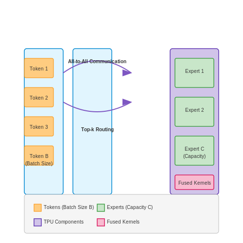
Efficient MoE routing requires careful coordination between computation and communication. The expert capacity factor C determines the maximum number of tokens an expert can process per batch, avoiding memory overflow. For a system with E experts and batch size B, the expected load balancing constraint is:
where ri denotes the routing decision for token i. Modern implementations use hierarchical all-to-all communication patterns, where devices first scatter tokens to expert partitions then gather results after processing.
Hardware-Software Co-Design
Specialized hardware accelerators like TPUs optimize MoE execution through:
- Fused expert kernel operations reducing memory bandwidth pressure
- Hardware-supported top-k routing with low-latency score sorting
- Sparse gradient accumulation for efficient backpropagation
The Megablocks framework demonstrates how CUDA kernel fusion can achieve 3-5× speedups over naive PyTorch implementations by eliminating intermediate memory allocations during expert routing.
Latency-Aware Routing
Production systems often augment the standard gating function with real-time performance metrics:
where ĝe estimates expert e's current processing latency. This prevents overloading slower experts while maintaining model quality. The hyperparameter λ controls the tradeoff between load balancing and computational efficiency.
Fault Tolerance Considerations
At data center scale, expert failures must not disrupt the entire model. Techniques include:
- Shadow experts that activate when primary experts time out
- Dynamic expert dropout during network congestion
- Graceful degradation via importance-weighted expert skipping
These mechanisms allow MoE models to maintain >99.9% availability despite individual expert failures, crucial for always-on services like machine translation and recommendation systems.
5. Latency and Computational Overhead
5.1 Latency and Computational Overhead
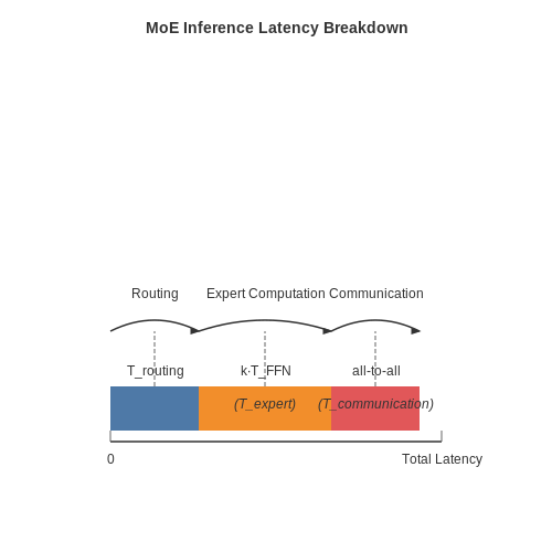
Sparse Mixture-of-Experts (MoE) models achieve computational efficiency by activating only a subset of experts per input, but this routing mechanism introduces unique latency considerations. The total inference time T can be decomposed as:
Routing Latency Breakdown
The routing overhead Trouting consists of:
- Gating computation: The forward pass through the gating network to compute expert selection probabilities. For a gating network with L layers and hidden dimension d, this requires O(Ld2) operations.
- Top-k selection: The sorting operation to select top-k experts from N candidates has O(N log N) complexity when using efficient partial sorting algorithms.
Expert Computation Costs
The activated expert computation Texpert scales with:
where TFFN is the latency of a single feed-forward network. While this remains constant per token, the aggregate expert computation across all devices introduces synchronization points in distributed settings.
Communication Bottlenecks
The all-to-all communication pattern in distributed MoE implementations creates a latency component:
where α is the fixed network latency, β is the inverse bandwidth, B is the batch size, and P is the number of partitions. This becomes dominant at scale, with measurements showing communication can consume 40-60% of total step time in large clusters.
Optimization Strategies
Recent approaches mitigate these overheads through:
- Hierarchical gating: Two-level routing that first selects device groups then local experts, reducing cross-device communication
- Expert caching: Predictive prefetching of likely expert parameters based on input characteristics
- Sparse all-to-all: Compression techniques like gradient sparsification applied to expert inputs/outputs
Empirical measurements on TPUv4 show these optimizations can reduce routing overhead from 28% to under 12% of total latency while maintaining model quality.
5.2 Fairness and Bias in Expert Selection
In sparse Mixture-of-Experts (MoE) models, the routing mechanism determines which subset of experts processes each input. While this improves computational efficiency, it introduces potential fairness and bias concerns. If certain experts are consistently underutilized or overutilized, the model may develop systemic biases, leading to uneven performance across different input domains or demographic groups.
Sources of Bias in Expert Routing
Bias in expert selection can arise from multiple sources:
- Imbalanced Training Data: If the training data disproportionately represents certain classes or features, the router may learn to favor experts specialized in those overrepresented patterns.
- Expert Capacity Constraints: Experts with limited capacity may become saturated, forcing the router to redirect inputs to less optimal experts, even if they are ill-suited for the task.
- Gradient Dominance: During training, gradients from high-frequency patterns may dominate updates, causing the router to prioritize experts handling those patterns.
Quantifying Fairness in Routing
To measure fairness, we define a routing distribution disparity metric:
where \( r_i \) is the routing frequency for expert \( i \), \( \bar{r} \) is the mean routing frequency, and \( N \) is the total number of experts. A higher \( D \) indicates greater imbalance.
Mitigation Strategies
Several approaches can reduce bias in expert selection:
- Load Balancing: Penalize the router when experts exceed a predefined capacity threshold, encouraging more uniform utilization.
- Adversarial Training: Introduce an adversarial loss term that discourages correlation between routing decisions and sensitive attributes (e.g., demographic features).
- Expert Dropout: Randomly disable experts during training to force the router to distribute inputs more evenly.
Case Study: Fair Routing in Multilingual Models
In multilingual MoE models, certain language-specific experts may dominate if high-resource languages (e.g., English) are overrepresented. A reweighting strategy can ensure balanced routing:
where \( w_l \) is the weight for language \( l \), \( f_l \) is its frequency in the training data, and \( \epsilon \) is a small constant for numerical stability. This downweights overrepresented languages, promoting fairer expert selection.
Practical Implications
Unchecked bias in routing can lead to:
- Degraded performance on minority classes or underrepresented data domains.
- Unintended discrimination in applications like hiring or loan approval systems.
- Reduced model robustness when expert specialization becomes overly narrow.
Emerging Research Frontiers
Dynamic Expert Capacity Allocation
Traditional sparse MoE models allocate fixed capacity per expert, leading to inefficiencies when input distributions are imbalanced. Recent work proposes dynamic capacity allocation, where the number of tokens assigned to each expert adapts based on routing probabilities. The routing function computes a softmax over expert scores, but instead of a fixed top-k, the capacity Ci for expert i is determined by:
where Ctotal is the total system capacity and si is the score for expert i. This approach reduces computational waste while maintaining load balancing.
Differentiable Routing with Entropy Regularization
Hard top-k routing is non-differentiable, complicating end-to-end training. Emerging solutions employ Gumbel-Softmax tricks or entropy-regularized objectives to smooth the routing process. The loss function L is augmented with an entropy term:
where H(p(x)) is the entropy of routing probabilities for input x, encouraging exploration across experts. This mitigates expert collapse—where a few experts dominate training—while preserving sparsity.
Hardware-Aware Routing Optimization
Efficient deployment on TPUs/GPUs requires minimizing cross-device communication. Research now optimizes routing to maximize locality, grouping tokens processed by the same expert onto the same device. The routing objective becomes:
where D is the number of devices and ℰd is the set of experts on device d. This reduces synchronization overhead, critical for large-scale models like Google’s Switch Transformer.
Multi-Objective Routing
Beyond accuracy, routing must optimize for latency, energy, and fairness. Pareto-optimal routing formulations weigh multiple objectives:
where ft are objective functions (e.g., FLOPs, memory access) and wt are learnable weights. This is particularly relevant for edge devices with strict resource constraints.
Cross-Modality Expert Specialization
In multimodal models (e.g., vision-language), experts can specialize in processing specific modalities. Routing dynamically selects modality-specific or cross-modal experts based on input type. The score function extends to:
where α is a learned mixing coefficient. This approach underpins models like Facebook’s FLAVA.
6. Key Research Papers
6.1 Key Research Papers
- PDF Do Experts Specialize? A Mechanistic Exploration of Mixture of Experts ... — Abstract A large number of prominent large-language-models have, over the past few years, adopted the Mixture of Ex-perts architecture to great success. These models, which seek to increase the parameter to compute ratio use multi-ple sparse MLPs, called experts, instead of a single dense MLP. A classic conception, given the name "experts" is that experts specialize in a subject much the ...
- PDF MegaBlocks: Efficient Sparse Training with Mixture-of-Experts — ABSTRACT We present MegaBlocks, a system for eficient Mixture-of-Experts (MoE) training on GPUs. Our system is motivated by the limitations of current frameworks, which restrict the dynamic routing in MoE layers to satisfy the constraints of existing software and hardware. These formulations force a tradeoff between model quality and hardware eficiency, as users must choose between dropping ...
- PDF Read-ME: Refactorizing LLMs as Router-Decoupled Mixture of Experts with ... — An Mixture-of-Expert (MoE) [1, 2, 17, 3] layer consists of a routing network G and a set of N expert networks {F1, ..., FN}. In the forward pass, the routing network will first process input sequences and generate the gating weights.
- Route, Select, Activate: The Mechanics of Mixture of Experts — Route, Select, Activ ate: The Mechanics of Mixture of Experts F awzi Gamal 1 1 Department of Computer Science and Technology, King Abdullah University of Science and T echnology Email: fawzi.gamal ...
- [2401.04088] Mixtral of Experts - arXiv.org — We introduce Mixtral 8x7B, a Sparse Mixture of Experts (SMoE) language model. Mixtral has the same architecture as Mistral 7B, with the difference that each layer is composed of 8 feedforward blocks (i.e. experts). For every token, at each layer, a router network selects two experts to process the current state and combine their outputs. Even though each token only sees two experts, the ...
- CompeteSMoE - Effective Sparse Mixture of Experts Training via Competition — Abstract Sparse mixture of experts (SMoE) offers an appealing solution to scale up the model complexity beyond the mean of increasing the network's depth or width. However, effective training of SMoE has proven to be challenging due to the representation collapse issue, which causes parameter redundancy and limited representation potentials. In this work, we propose a competition mechanism ...
- (PDF) Sparsely Activated Mixture-of-Experts are Robust Multi-Task ... — This results in a sparsely activated multi-task model with a large number of parameters, but with the same computational cost as that of a dense model. We demonstrate such sparse networks to improve multi-task learning along three key dimensions: (i) transfer to low-resource tasks from related tasks in the training mixture; (ii) sample-eff...
- Overcoming language barriers via machine translation with sparse ... — In this paper, we introduce MoE-LLM, a novel fusion framework that enhances the multilingual translation abilities of LLMs by incorporating sparse Mixture-of-Experts (MoEs) components via hybrid transfer learning. MoE-LLM freezes the LLM parameters, mitigating forgetting, and introduces specialized translation experts within the MoEs modules.
- Improving Deep Learning Performance with Mixture of Experts and Sparse ... — The increasing complexity and scale of modern machine learning models have led to growing computational demands, raising concerns about efficiency, scalability, and adaptability. Traditional deep learning architectures often struggle to balance computational cost with model expressiveness, particularly in tasks requiring specialization across diverse data distributions. One promising solution ...
- Training Sparse Mixture Of Experts Text Embedding Models — In this paper, we target this issue by assembling niche datasets using co-citations as a similarity metric, focusing on biomedical domains. We employ two key strategies for fine-tuning state-of ...
6.2 Open-Source Implementations
- GitHub - XueFuzhao/OpenMoE: A family of open-sourced Mixture-of-Experts ... — OpenMoE is a project aimed at igniting the open-source MoE community! We are releasing a family of open-sourced Mixture-of-Experts (MoE) Large Language Models. Our project began in the summer of 2023. On August 22, 2023, we released the first batch of intermediate checkpoints (OpenMoE-base&8B), along with the data and code . Subsequently, the ...
- FSMoE: A Flexible and Scalable Training System for Sparse Mixture-of ... — put tokens is still an open problem, which means the routing function plays an important role in the model generalization capability [6, 12, 22, 23, 36, 40, 51]. ... implementations. •Based on the modularized operations, we propose an ... A Flexible and Scalable Training System for Sparse Mixture-of-Experts Models ASPLOS '25, March 30-April ...
- PDF MegaBlocks: Efficient Sparse Training with Mixture-of-Experts - MLSys — learned routing algorithm described above provides no guar-antees of a load balanced assignment of tokens to experts. In order to satisfy this constraint, prior work has defined a fixed expert capacity, which is the number of tokens that each expert can be assigned (Lepikhin et al.(2020);Fedus et al.(2022)). If the number of tokens assigned to ...
- PDF TUTEL: ADAPTIVE MIXTURE OF-EXPERTS AT SCALE - MLSys — source and energy cost (Sharir et al.,2020). To tackle this, sparsely-gated Mixture-of-Experts (MoE) (Shazeer et al., 2017) introduces a sparse architecture by employing mul-tiple parallel sub-models called experts, where each input is only forwarded to a few experts based on an intelligent gating function. Unlike dense layers, this method scales
- Mixture-of-Experts: a publications timeline, with serial and ... — The current state-of-art MoE model is the Mixtral 8x7B, a sparse mixture of expert, with the same architecture as Mixtral 7B except that it supports a fully dense context length of 32k tokens and the feed-forward blocks are replaced by a Mixture of 8 feed-forward network experts. Model architecture is detailed in Table 1.
- FSMoE: A Flexible and Scalable Training System for Sparse Mixture-of ... — Experimental results show that 1) our FSMoE supports four popular types of MoE routing functions and is more efficient than existing implementations (with up to a 1.42 × \times × speedup), and 2) FSMoE outperforms the state-of-the-art MoE training systems (DeepSpeed-MoE and Tutel) by 1.18 × \times ×-1.22 × \times × on 1458 MoE layers and ...
- Mixture-of-Experts (MoE): The Birth and Rise of Conditional ... - Substack — The router has its own set of parameters and is trained jointly with the rest of the network. Each token can be sent to many experts, but we impose sparsity by only sending a token to its top-K experts.For example, many models set k=1 or k=2, meaning that each token is processed by either one or two experts, respectively.. Greater capacity, fixed computation.
- GitHub - microsoft/Tutel: Tutel MoE: Optimized Mixture-of-Experts ... — parallel_type : the parallel method to compute MoE, valid types: 'auto', 'data', 'model' pad_samples : whether do auto padding on newly-coming input data to maximum data size in history * Usage of dict-type Experts Config: num_experts_per_device : the number of local experts per device (by default, the value is 1 if not specified) hidden_size ...
- Overcoming language barriers via machine translation with sparse ... — One promising approach to address these challenges is the integration of Mixture-of-Experts (MoEs) within the NMT framework. MoE is a powerful neural network architecture designed to improve performance and efficiency, especially when dealing with complex and diverse data (Fedus, Zoph, & Shazeer, 2022).It operates by leveraging multiple specialized sub-networks, called experts, each focusing ...
- Training Sparse Mixture Of Experts Text Embedding Models - ResearchGate — The Mixture of Experts (MoE) architecture was first intro- duced by Shazeer et al. ( 2017 ) as a method to increase model capacity and performance without a proportional increase
6.3 Recommended Tutorials and Surveys
- PDF Language-Routing Mixture of Experts for Multilingual and Code-Switching ... — Gated Mixture of Experts (sMoE), (b) Mixture of Language Ex-perts (MLE). 3. Proposed Method 3.1. Sparsely-Gated Mixture of Experts The sMoE module is shown in Fig. 1(a). As a representative, Switch Transformer [27] adopts a top-1 expert routing strategy in the MoE architecture to route the data samples to the ex-
- CompeteSMoE - Effective Sparse Mixture of Experts Training via Competition — To go beyond simply increasing the network depth and width, Sparse Mixture-of-experts (SMoE) (Fedus et al., 2022) has risen as an appealing solution for scaling LLMs. By modularizing the network and activating only subsets of experts per input, SMoE offers constant computational costs while scaling up the model complexity, which often results ...
- Mixture-of-Experts: a publications timeline, with serial and ... — The current state-of-art MoE model is the Mixtral 8x7B, a sparse mixture of expert, with the same architecture as Mixtral 7B except that it supports a fully dense context length of 32k tokens and the feed-forward blocks are replaced by a Mixture of 8 feed-forward network experts. Model architecture is detailed in Table 1.
- PDF Mod-Squad: Designing Mixtures of Experts As Modular Multi-Task Learners — a subset of experts that learn specific features (as needed by some tasks) and do not interfere with each other (spe-cialization). Such an assignment of tasks to experts can be represented via a sparse but strong dependence between experts and tasks. Fig.1illustrates this key difference be-tween our model and previous MoE work, showing how our
- MegaBlocks: Efficient Sparse Training with Mixture-of-Experts - arXiv.org — Figure 1. A Mixture-of-Experts Layer. Shown for num experts=3, top k=1 and capacity factor=1 with the prevalent, token dropping formulation. First (1), tokens are mapped to experts by the router. Along with expert assignments, the router produces probabilities that reflect the confidence of the assignments.
- PDF MegaBlocks: Efficient Sparse Training with Mixture-of-Experts - MLSys — learned routing algorithm described above provides no guar-antees of a load balanced assignment of tokens to experts. In order to satisfy this constraint, prior work has defined a fixed expert capacity, which is the number of tokens that each expert can be assigned (Lepikhin et al.(2020);Fedus et al.(2022)). If the number of tokens assigned to ...
- From Sparse to Soft Mixtures of Experts - arXiv.org — Sparse MoE Transformers involve a discrete optimization problem to decide which modules should be applied to each token. These modules are commonly referred to as experts and are usually MLPs. Many techniques have been devised to find good token-to-expert matches: linear programs (Lewis et al., 2021), reinforcement learning (Bengio et al., 2015), deterministic fixed rules (Roller et al., 2021 ...
- Reinforcement Learning for Quantitative Trading — To the best of our knowledge, this survey is the first comprehensive survey on RL-based quantitative trading applications. ... An efficient Mixture-of-Experts framework ... Shuo Sun, Rundong Wang, and Bo An. 2022. Quantitative stock investment by routing uncertainty-aware trading experts: A multi-task learning approach. arXiv preprint arXiv ...
- A review of clustering techniques and developments — A useful tutorial is available on spectral clustering by Luxburg [181]. The success of spectral clustering is mainly based on the fact that it does not make strong assumptions on the form of the clusters. ... as long as we make sure that the similarity graph is sparse. Once the similarity graph is chosen, we just have to solve a linear problem ...
- Foundations & Trends in Multimodal Machine Learning: Principles ... — This survey was also presented by the authors in a visual medium through tutorials at CVPR 2022 and NAACL 2022, as well as courses 11-777 Multimodal Machine Learning and 11-877 Advanced Topicsin Multimodal Machine Learning at CMU. The reader is encouraged to refer to these public video recordings, additional readings, and discussion probes for ...