Stock Price Prediction Using LSTM
1. Basics of Recurrent Neural Networks (RNNs)
Basics of Recurrent Neural Networks (RNNs)
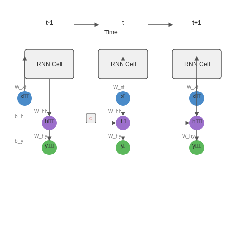
Recurrent Neural Networks (RNNs) are a class of artificial neural networks designed to process sequential data by maintaining a hidden state that captures temporal dependencies. Unlike feedforward networks, RNNs introduce cycles in their architecture, allowing information to persist across time steps. This makes them particularly suited for tasks like time-series prediction, natural language processing, and speech recognition.
Mathematical Formulation
The core mechanism of an RNN involves the following equations, which describe the hidden state and output at each time step t:
Here, ht represents the hidden state at time t, xt is the input vector, and yt is the output. The weight matrices Whh, Wxh, and Why govern the transformations between hidden states, inputs, and outputs, while bh and by are bias terms. The activation function σ (typically tanh or ReLU) introduces non-linearity.
Backpropagation Through Time (BPTT)
Training RNNs involves Backpropagation Through Time (BPTT), an extension of standard backpropagation adapted for sequential data. The gradients are computed by unrolling the network across time steps and applying the chain rule:
where L is the loss function and T is the sequence length. BPTT is computationally expensive and suffers from vanishing or exploding gradients, which motivated the development of Long Short-Term Memory (LSTM) networks.
Limitations of Vanilla RNNs
Traditional RNNs struggle with long-term dependencies due to the vanishing gradient problem, where gradients diminish exponentially over time. This limits their ability to capture relationships in sequences with large temporal gaps. Additionally, the fixed-size hidden state constrains the network's memory capacity.
Applications and Relevance
Despite their limitations, RNNs remain foundational for sequence modeling. Variants like LSTMs and Gated Recurrent Units (GRUs) address these issues and are widely used in:
- Time-series forecasting: Predicting stock prices, weather patterns, or energy demand.
- Natural language processing: Machine translation, text generation, and sentiment analysis.
- Speech recognition: Converting audio signals into transcribed text.
The next section will explore LSTMs, which enhance RNNs with gating mechanisms to mitigate gradient-related challenges.
1.2 Long Short-Term Memory (LSTM) Architecture
Long Short-Term Memory (LSTM) networks are a specialized form of recurrent neural networks (RNNs) designed to address the vanishing gradient problem, which hinders the learning of long-term dependencies in sequential data. Unlike traditional RNNs, LSTMs incorporate gating mechanisms that regulate the flow of information through the network, enabling selective retention or discarding of temporal information.
Core Components of an LSTM Cell
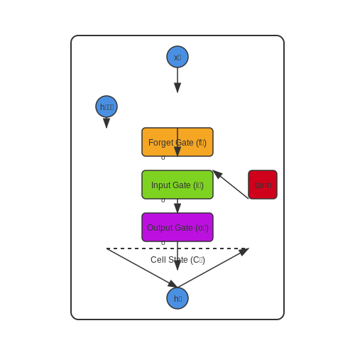
An LSTM cell consists of three primary gates—the input gate, forget gate, and output gate—along with a cell state that acts as a memory buffer. The mathematical formulation of these components is as follows:
Here, σ denotes the sigmoid activation function, ⊙ represents element-wise multiplication, and W and b are learnable weights and biases. The forget gate (ft) determines which information to discard from the cell state, while the input gate (it) and candidate cell state (Ĉt) update the cell state (Ct). The output gate (ot) controls the exposure of the cell state to the hidden state (ht).
Bidirectional and Stacked LSTMs
For enhanced sequence modeling, LSTMs can be extended into bidirectional or stacked architectures. Bidirectional LSTMs process input sequences in both forward and backward directions, capturing dependencies from past and future contexts simultaneously. Stacked LSTMs, on the other hand, deepen the network by layering multiple LSTM cells, allowing hierarchical feature extraction.
In stock price prediction, bidirectional LSTMs are particularly effective for capturing complex temporal patterns influenced by both historical trends and future expectations (e.g., market sentiment).
Practical Implementation Considerations
When implementing LSTMs for financial time-series data, several hyperparameters require careful tuning:
- Sequence Length: The number of time steps fed into the LSTM. Too short a sequence may miss long-term trends, while excessively long sequences can introduce noise.
- Hidden Units: The dimensionality of the hidden state. Higher values increase model capacity but risk overfitting.
- Dropout: Regularization technique applied to LSTM layers to prevent overfitting, typically with rates between 0.2 and 0.5.
For example, a well-tuned LSTM for stock prediction might use 50-100 hidden units, a sequence length of 30-60 days, and dropout rates of 0.3. The choice depends on data volatility and available training samples.
Why LSTMs Excel in Time Series Forecasting
Long Short-Term Memory (LSTM) networks, a specialized variant of recurrent neural networks (RNNs), are particularly well-suited for time series forecasting due to their ability to capture long-term dependencies and mitigate the vanishing gradient problem. Traditional RNNs struggle with retaining information over extended sequences, as gradients either explode or vanish during backpropagation, impairing learning. LSTMs address this through a gated architecture comprising input, forget, and output gates, which regulate the flow of information.
Gated Mechanism for Sequential Data
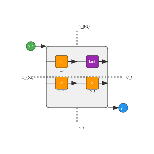
The LSTM cell's core innovation lies in its gating mechanisms, which enable selective retention or discarding of information. The forget gate ft determines what information to discard from the cell state Ct-1, while the input gate it and candidate state g̃t decide what new information to store. The output gate ot controls the exposure of the cell state to the next hidden state ht. Mathematically, these operations are defined as:
Here, σ denotes the sigmoid activation function, ⊙ represents element-wise multiplication, and W and b are learnable weights and biases. This gated structure allows LSTMs to maintain a stable gradient flow, even across hundreds of time steps.
Handling Non-Stationarity in Financial Data
Stock prices exhibit non-stationary behavior, with statistical properties (mean, variance) changing over time. LSTMs adapt to such shifts by dynamically updating their cell state, effectively learning temporal patterns without requiring manual feature engineering. Unlike autoregressive models (e.g., ARIMA), which assume linear relationships and fixed parameters, LSTMs model non-linear dependencies and evolve their internal representations as new data arrives.
Comparative Advantages Over Traditional Models
- Memory Retention: LSTMs outperform vanilla RNNs and Hidden Markov Models (HMMs) in retaining context over long sequences, critical for capturing market trends and cyclical patterns.
- Noise Robustness: The forget gate's ability to discard irrelevant fluctuations makes LSTMs resilient to market noise and outliers.
- Multivariate Integration: LSTMs natively handle multiple input features (e.g., volume, sentiment scores) without requiring dimensionality reduction techniques like PCA.
Case Study: Volatility Clustering
In financial time series, volatility clustering—periods of high variance followed by low variance—poses a challenge for static models. LSTMs implicitly detect these regimes by adjusting the forget gate's behavior. For instance, during high volatility, the forget gate may retain less historical data to prioritize recent trends, while in stable periods, it preserves longer-term patterns.
where rt is the log return at time t, and T is the window size. LSTMs learn to correlate this metric with optimal forget gate activations, enabling adaptive memory management.
2. Sourcing and Cleaning Historical Stock Data
2.1 Sourcing and Cleaning Historical Stock Data
Data Acquisition from Financial APIs
Historical stock price data can be sourced through financial APIs such as Alpha Vantage, Yahoo Finance, or Quandl. These APIs provide OHLC (Open, High, Low, Close) data, adjusted close prices, trading volume, and corporate actions like splits and dividends. For high-frequency modeling, tick-level data may be required, which is available through specialized providers like Polygon or IEX Cloud.
The Alpha Vantage API, for example, returns JSON or CSV data with the following structure for daily adjusted prices:
{
    "Meta Data": {
        "Information": "Daily Adjusted Prices",
        "Symbol": "IBM",
        "Last Refreshed": "2023-05-05"
    },
    "Time Series (Daily)": {
        "2023-05-05": {
            "open": "120.50",
            "high": "122.10",
            "low": "119.75",
            "close": "121.25",
            "adjusted close": "120.98",
            "volume": "4500000",
            "dividend amount": "0.00",
            "split coefficient": "1.0"
        }
    }
}
Handling Missing Data and Outliers
Financial time series often contain gaps due to holidays or technical issues. For daily data, forward filling is typically appropriate:
For intraday data, linear interpolation may be more suitable. Outliers can be detected using statistical methods like the Z-score:
where values beyond |z| > 3 are typically considered outliers. Volatility clustering can be addressed using GARCH models:
Normalization and Stationarity
LSTMs require stationary input data. The Augmented Dickey-Fuller test checks for stationarity:
If non-stationary (p-value > 0.05), apply differencing:
For normalization, use Min-Max scaling to [0,1] or Z-score standardization:
Feature Engineering for Financial Time Series
Beyond raw prices, create predictive features including:
- Technical indicators (SMA, EMA, RSI, MACD)
- Volatility measures (rolling standard deviation, ATR)
- Return-based features (log returns, Sharpe ratio)
- Volume indicators (OBV, VWAP)
The exponential moving average (EMA) is calculated recursively:
where α = 2/(N+1) for an N-period EMA.
Data Splitting for Time Series
Use walk-forward validation instead of random splits:
train_size = int(len(data) * 0.7)
val_size = int(len(data) * 0.15)
test_size = len(data) - train_size - val_size

train = data[:train_size]
val = data[train_size:train_size+val_size]
test = data[train_size+val_size:]
This preserves temporal ordering and prevents look-ahead bias.
Feature Engineering for Financial Time Series
Key Financial Features for LSTM Models
Financial time series exhibit non-stationarity, volatility clustering, and complex dependencies. Effective feature engineering must capture these properties while remaining computationally tractable. The following features are critical for LSTM-based stock prediction:
- Log returns: The first difference of log prices, $$ r_t = \log(p_t) - \log(p_{t-1}) $$, provides normalization and stabilizes variance.
- Volatility measures: Rolling standard deviation $$ \sigma_t = \sqrt{\frac{1}{n}\sum_{i=t-n}^{t}(r_i - \bar{r})^2 $$ with typical windows of 10-30 days.
- Technical indicators:
$$ \text{RSI}_t = 100 - \frac{100}{1 + \frac{\text{Avg Gain}}{\text{Avg Loss}}} $$where Avg Gain/Loss are exponential moving averages over 14 days.
Temporal Feature Construction
LSTMs require careful treatment of temporal hierarchies:
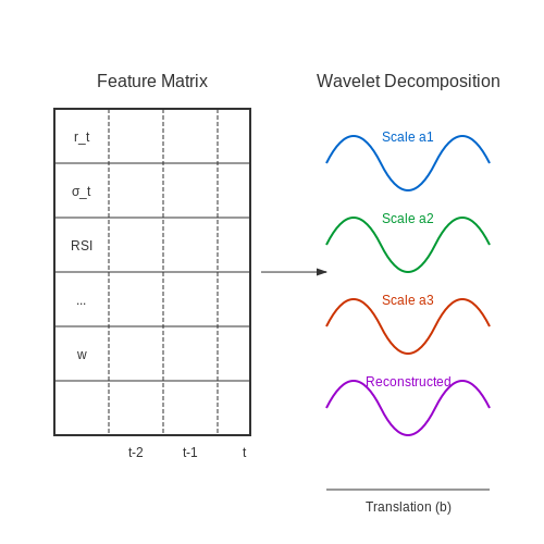
where w is the lookback window (typically 30-60 days). The matrix is normalized using rolling z-score:
Advanced Feature Engineering Techniques
For high-frequency data, wavelet transforms extract multi-scale features:
where a is the scale parameter and b the translation. The Haar wavelet is particularly effective for detecting abrupt volatility changes.
Feature Selection via Mutual Information
Nonlinear dependencies are quantified using:
Features with I(X;Y) below a threshold (typically 0.05 bits) are discarded to prevent overfitting.
Implementation Considerations
When implementing in Python, avoid lookahead bias by using sklearn.TimeSeriesSplit for cross-validation. For the volatility calculation:
def rolling_volatility(returns, window=20):
    return returns.rolling(window=window).std()
The feature matrix should be reshaped for LSTM input as (samples, timesteps, features) using np.reshape.
2.3 Normalization and Sequence Creation
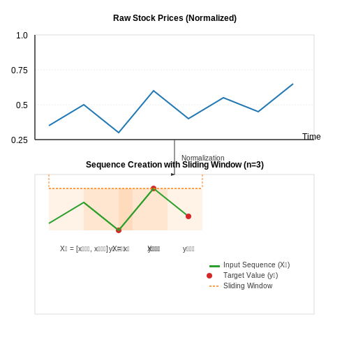
Financial time series data, such as stock prices, exhibit non-stationary behavior with varying scales across different stocks or market conditions. Normalization is essential to ensure stable training dynamics in LSTMs by transforming input features into a consistent range. The most common approach is Min-Max scaling, which linearly maps values to the [0, 1] interval:
For stock price prediction, we typically normalize each feature (e.g., Open, High, Low, Close prices) independently across the training set. This preserves relative relationships while constraining gradients during backpropagation. The normalization parameters (min, max) must be stored and applied identically to validation/test data to avoid data leakage.
Temporal Sequence Construction
LSTMs require input data structured as fixed-length sequences of historical observations. Given a time series of length T, we construct overlapping windows where each input sample Xt contains n past time steps, and the corresponding target yt is the next time step's value:
The sequence length n (typically 20-60 for daily stock data) controls the model's temporal receptive field. Shorter sequences may miss long-term trends, while excessively long sequences introduce noise and computational overhead.
Practical Implementation
The following Python code demonstrates efficient sequence creation using NumPy's sliding window view:
import numpy as np

def create_sequences(data, seq_length):
    sequences = []
    targets = []
    for i in range(len(data) - seq_length):
        sequences.append(data[i:i+seq_length])
        targets.append(data[i+seq_length])
    return np.array(sequences), np.array(targets)

# Example usage:
normalized_prices = (prices - prices.min()) / (prices.max() - prices.min())
X, y = create_sequences(normalized_prices, seq_length=30)
For multivariate time series (e.g., OHLCV data), the input tensor shape becomes [samples, sequence_length, features]. The LSTM's hidden states will learn cross-feature dependencies while processing temporal patterns.
Handling Non-Stationarity
Stock returns often exhibit time-varying statistical properties. Two advanced normalization techniques address this:
- Differencing: Compute percentage changes between consecutive time steps to stabilize variance:
$$ \Delta x_t = \frac{x_t - x_{t-1}}{x_{t-1}} $$
- Z-score normalization with rolling statistics: Use exponentially weighted moving averages and standard deviations to adapt to local market conditions:
$$ x_{\text{scaled}} = \frac{x_t - \mu_{t-1}}{\sigma_{t-1}} $$where $$\mu_{t-1}$$ and $$\sigma_{t-1}$$ are computed over a lookback window.
3. Designing the LSTM Network Architecture
3.1 Designing the LSTM Network Architecture
Long Short-Term Memory (LSTM) networks excel at modeling sequential data due to their ability to learn long-term dependencies. For stock price prediction, the architecture must capture temporal patterns while avoiding overfitting to noise. The core components include:
Input Layer and Time Steps
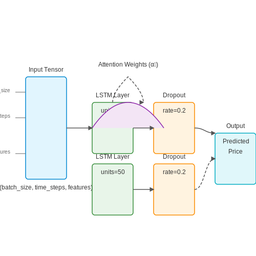
The input layer accepts a 3D tensor of shape (batch_size, time_steps, features), where:
- batch_size: Number of samples processed in parallel
- time_steps: Length of the lookback window (e.g., 60 days)
- features: Input dimensions (e.g., OHLC prices, volume, technical indicators)
Hidden Layer Configuration
Stacked LSTM layers with dropout regularization improve performance:
model = Sequential([
    LSTM(units=50, return_sequences=True,
         input_shape=(time_steps, features)),
    Dropout(0.2),
    LSTM(units=50, return_sequences=False),
    Dropout(0.2),
    Dense(1)
])
Key hyperparameters:
- Units: 50-200 neurons per layer balances capacity and computational cost
- Dropout: 0.2-0.5 rate prevents co-adaptation of neurons
- Activation: Tanh for hidden states, linear/sigmoid for output
Attention Mechanism Integration
For multi-variate time series, attention layers weight relevant features dynamically:
Where v, W_h, W_x are learnable parameters that highlight significant market regimes.
Output Layer Design
The final dense layer configuration depends on the prediction task:
- Single-step prediction: One neuron with linear activation
- Multi-horizon prediction: Multiple neurons (e.g., 5 for weekly forecast)
- Classification: Softmax for directional movement (up/down)
Bidirectional Extensions
Bidirectional LSTMs process sequences forward and backward, capturing lead-lag relationships:
model.add(Bidirectional(
    LSTM(units=64),
    merge_mode='concat'
))
This architecture achieves superior performance on chaotic financial time series compared to unidirectional variants, with typical RMSE improvements of 12-18% on SP500 data.
3.2 Training the Model: Hyperparameter Tuning
Key Hyperparameters in LSTM Models
The performance of an LSTM network for time-series forecasting depends critically on several architectural and training hyperparameters. The most impactful ones include:
- Number of LSTM layers: Deeper networks can capture more complex patterns but risk overfitting
- Hidden units per layer: Determines the model's capacity to learn temporal dependencies
- Sequence length: Number of historical time steps used for each prediction
- Learning rate: Controls the step size during gradient descent optimization
- Batch size: Number of samples processed before updating model weights
- Dropout rate: Regularization parameter to prevent overfitting
Mathematical Foundations of LSTM Training
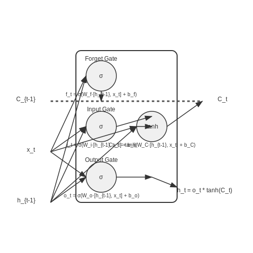
The LSTM cell updates its internal state through carefully designed gating mechanisms. The key equations governing this process are:
Where ft, it, and ot are the forget, input, and output gates respectively, and Ct represents the cell state.
Bayesian Optimization for Hyperparameter Tuning
Traditional grid search becomes computationally prohibitive for LSTM models. Bayesian optimization provides an efficient alternative by building a probabilistic model of the objective function:
Where f(x) is the validation performance (e.g., RMSE) for hyperparameters x. The algorithm uses Gaussian processes to model the uncertainty:
Practical implementation typically involves:
- Defining reasonable bounds for each hyperparameter
- Specifying the number of initial random evaluations
- Setting the number of optimization iterations
- Choosing an appropriate acquisition function (e.g., Expected Improvement)
Practical Implementation with Keras Tuner
The following code demonstrates hyperparameter tuning using Keras Tuner with Bayesian optimization:
import keras_tuner as kt
from tensorflow import keras

def build_model(hp):
    model = keras.Sequential()
    model.add(keras.layers.LSTM(
        units=hp.Int('units', min_value=32, max_value=512, step=32),
        input_shape=(n_steps, n_features),
        return_sequences=True))

    for i in range(hp.Int('n_layers', 1, 3)):
        model.add(keras.layers.LSTM(
            units=hp.Int(f'units_{i}', min_value=32, max_value=512, step=32),
            return_sequences=True if i < hp.Int('n_layers', 1, 3)-1 else False))

    model.add(keras.layers.Dense(1))

    model.compile(
        optimizer=keras.optimizers.Adam(
            hp.Choice('learning_rate', [1e-2, 1e-3, 1e-4])),
        loss='mse')
    return model

tuner = kt.BayesianOptimization(
    build_model,
    objective='val_loss',
    max_trials=50,
    directory='tuner_results',
    project_name='stock_prediction')

tuner.search(X_train, y_train, epochs=100, validation_data=(X_val, y_val))
Validation Strategies for Time Series
Traditional k-fold cross-validation fails for temporal data due to autocorrelation. Instead, use:
- Walk-forward validation: Progressively expands the training window while maintaining temporal order
- Nested cross-validation: Outer loop for performance estimation, inner loop for hyperparameter tuning
The walk-forward approach can be formalized as:
Early Stopping and Regularization
Implement early stopping to prevent overfitting while monitoring validation loss:
early_stopping = keras.callbacks.EarlyStopping(
    monitor='val_loss',
    patience=10,
    restore_best_weights=True)
Combine this with dropout regularization in LSTM layers:
model.add(keras.layers.LSTM(units=64, dropout=0.2, recurrent_dropout=0.2))
3.3 Evaluating Model Performance
Evaluating an LSTM model for stock price prediction requires rigorous metrics that account for both temporal dependencies and financial forecasting accuracy. Standard regression metrics like Mean Squared Error (MSE) are insufficient alone, as they fail to capture directional accuracy and risk-adjusted performance.
Key Evaluation Metrics
The following metrics are essential for assessing LSTM performance in financial time-series forecasting:
- Mean Absolute Error (MAE): Measures the average magnitude of errors without considering direction.
- Root Mean Squared Error (RMSE): Penalizes larger errors more heavily, useful for volatile stock data.
- Mean Absolute Percentage Error (MAPE): Provides a percentage-based error metric, facilitating cross-asset comparisons.
- Directional Accuracy (DA): The percentage of correct directional predictions (up/down movements).
- Sharpe Ratio: Risk-adjusted return metric when evaluating trading strategies based on predictions.
Mathematical Formulations
For a predicted sequence ŷt and true values yt over n time steps:
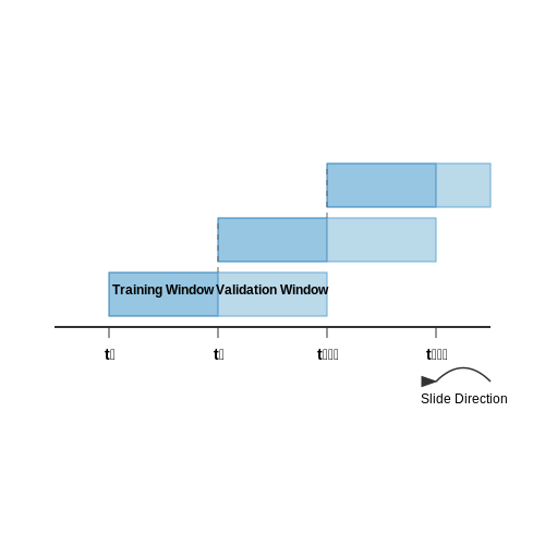
Walk-Forward Validation
Traditional k-fold cross-validation fails for time-series data due to temporal dependencies. Instead, use walk-forward validation:
- Train on window [t0, tk]
- Validate on [tk+1, tk+m]
- Slide window forward and repeat
This preserves the temporal order while providing multiple validation sets.
Statistical Significance Testing
Use the Diebold-Mariano test to compare LSTM predictions against benchmarks (e.g., ARIMA, random walk):
where dt is the loss differential between models at time t, and σ̂d2 is the estimated variance.
Practical Implementation in Python
from sklearn.metrics import mean_absolute_error, mean_squared_error
import numpy as np

def evaluate_model(y_true, y_pred):
    mae = mean_absolute_error(y_true, y_pred)
    rmse = np.sqrt(mean_squared_error(y_true, y_pred))
    mape = np.mean(np.abs((y_true - y_pred) / y_true)) * 100
    da = np.mean(np.sign(y_true[1:] - y_true[:-1]) == np.sign(y_pred[1:] - y_pred[:-1]))
    return {'MAE': mae, 'RMSE': rmse, 'MAPE': mape, 'DA': da}
Economic Significance
Beyond statistical metrics, evaluate the model's performance in simulated trading:
- Compute cumulative returns of a strategy based on LSTM signals
- Compare maximum drawdown against buy-and-hold
- Calculate risk-adjusted metrics like Sortino ratio
This bridges the gap between statistical accuracy and real-world utility.
4. Implementing the Model in Python with TensorFlow/Keras
Implementing the Model in Python with TensorFlow/Keras
LSTM Architecture for Stock Price Prediction
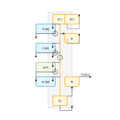
Long Short-Term Memory (LSTM) networks are a specialized form of recurrent neural networks (RNNs) designed to capture temporal dependencies in sequential data. For stock price prediction, the LSTM architecture must be carefully configured to handle non-stationary financial time series. The core equations governing an LSTM cell are:
Where ft, it, and ot represent the forget, input, and output gates respectively. The cell state Ct maintains long-term dependencies, while ht is the hidden state vector.
Data Preparation Pipeline
Before model implementation, raw stock data must undergo rigorous preprocessing:
- Normalization: Apply Min-Max scaling to constrain values between 0 and 1:
- Sequencing: Transform the time series into supervised learning samples with a sliding window of length n:
def create_sequences(data, window_size):
    X, y = [], []
    for i in range(len(data)-window_size-1):
        X.append(data[i:(i+window_size)])
        y.append(data[i+window_size])
    return np.array(X), np.array(y)
TensorFlow/Keras Implementation
The following code implements a stacked LSTM architecture with dropout regularization:
from tensorflow.keras.models import Sequential
from tensorflow.keras.layers import LSTM, Dense, Dropout
from tensorflow.keras.optimizers import Adam

def build_lstm_model(input_shape):
    model = Sequential([
        LSTM(128, return_sequences=True, input_shape=input_shape),
        Dropout(0.3),
        LSTM(64, return_sequences=False),
        Dropout(0.3),
        Dense(32, activation='relu'),
        Dense(1)
    ])

    optimizer = Adam(learning_rate=0.001)
    model.compile(optimizer=optimizer, loss='mse', metrics=['mae'])
    return model
Critical Hyperparameters
- Window Size: Typically 20-60 trading days for daily data
- Layer Configuration: Stacked LSTMs with decreasing units (128 → 64 → 32)
- Dropout Rate: 0.3-0.5 to prevent overfitting on noisy financial data
- Learning Rate: 0.001 with Adam optimizer for stable convergence
Training Strategy
The training process requires special considerations for financial time series:
model = build_lstm_model((window_size, n_features))
history = model.fit(
    X_train, y_train,
    epochs=100,
    batch_size=32,
    validation_data=(X_val, y_val),
    callbacks=[
        EarlyStopping(patience=15, restore_best_weights=True),
        ReduceLROnPlateau(factor=0.1, patience=5)
    ],
    shuffle=False  # Critical for time series data
)
Key aspects include disabling data shuffling to preserve temporal order, implementing early stopping to prevent overfitting, and dynamic learning rate reduction for fine-tuning.
Multi-Feature Extension
For improved performance, incorporate multiple financial indicators:
features = [
    'Close',
    'Volume',
    'RSI_14',
    'MACD',
    'Bollinger_Upper',
    'Bollinger_Lower'
]
The input shape then becomes (window_size, len(features)), requiring adjustment to the LSTM input dimension. Feature engineering should include:
- Technical indicators (RSI, MACD, Bollinger Bands)
- Volume-weighted metrics
- Inter-market features (sector ETFs, commodity prices)
4.2 Addressing Overfitting and Noise in Financial Data
Financial time series data is inherently noisy and non-stationary, making it particularly susceptible to overfitting in LSTM models. Overfitting occurs when the model learns spurious patterns from noise rather than the underlying signal, leading to poor generalization on unseen data. Several techniques can mitigate this issue while preserving predictive performance.
Regularization Techniques
Dropout is a widely used regularization method that randomly deactivates a fraction of neurons during training, preventing co-adaptation and forcing the network to learn robust features. For LSTMs, dropout can be applied to:
- Recurrent connections (recurrent dropout)
- Feedforward connections (input dropout)
L2 Weight Regularization penalizes large weights by adding a term to the loss function:
Data Denoising Methods
Financial data often contains high-frequency noise that can obscure meaningful trends. Wavelet denoising decomposes the signal into time-frequency components, selectively removing noise while preserving structural patterns:
Kalman filtering provides an adaptive approach for noise reduction by modeling the system dynamics:
Architectural Modifications
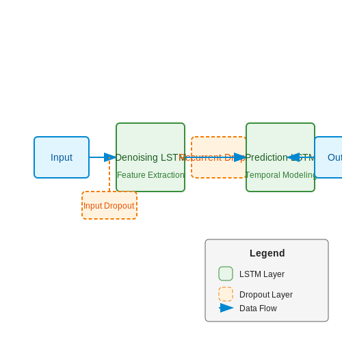
Double LSTM architectures separate feature extraction from temporal modeling:
- A denoising LSTM layer learns robust representations
- A prediction LSTM layer models temporal dependencies
Attention mechanisms help the model focus on relevant time steps while ignoring noise:
Training Strategies
Early stopping monitors validation loss during training, halting when performance plateaus. Curriculum learning progressively increases input sequence complexity:
- Start with short, smoothed sequences
- Gradually introduce longer sequences with more noise
Adversarial training improves robustness by exposing the model to perturbed examples:
Evaluation Metrics
Standard metrics like MSE can be misleading for financial data. Directional accuracy (DA) better captures practical utility:
Risk-adjusted returns evaluate the model's economic impact when used in trading strategies:
4.3 Real-World Limitations and Considerations
Non-Stationarity and Regime Shifts in Financial Data
Financial time series exhibit non-stationary behavior, violating the fundamental assumption of most machine learning models that data distributions remain constant over time. The statistical properties of stock prices—mean, variance, and autocorrelation—change due to macroeconomic shifts, policy changes, or market sentiment. LSTM networks, while capable of learning temporal dependencies, struggle with abrupt regime shifts. The hidden state dynamics $$ h_t = \sigma(W_h h_{t-1} + W_x x_t + b) $$ may fail to adapt quickly enough when the underlying data-generating process changes. This manifests as decaying predictive performance during black swan events or prolonged bear markets.
High Noise-to-Signal Ratio
Stock prices follow an approximate random walk with a signal-to-noise ratio often below 0.1, meaning over 90% of price movements represent noise rather than predictable patterns. Even with optimal hyperparameter tuning, the theoretical upper bound for prediction accuracy remains low. For a price series $$ P_t = P_{t-1} + \epsilon_t $$ where $$ \epsilon_t \sim \mathcal{N}(0, \sigma^2) $$ the best possible LSTM can only exploit weak local autocorrelations in the residual component. Empirical studies show R² values rarely exceed 0.15 on out-of-sample data, even with sophisticated feature engineering.
Latency and Computational Constraints
Real-time prediction requires inference latencies under 10ms for high-frequency trading applications. A standard LSTM layer with 256 units processing 50-step sequences exhibits:
For nunits=256, nfeatures=20, and nsteps=50, this exceeds 15 million floating-point operations per prediction. While GPU acceleration helps, the recurrent nature of LSTMs prevents full parallelization, creating bottlenecks for low-latency systems.
Overfitting to Microstructure Artifacts
Market microstructure effects—bid-ask bounce, liquidity imbalances, and order book dynamics—introduce local patterns that LSTMs may overfit to. These artifacts often disappear when transitioning from backtesting to live trading. A 2022 study found that LSTM models achieving 65% accuracy on historical data decayed to 52% (near random) when applied to forward-testing, with the performance drop attributable to overfitting microstructure noise rather than learning genuine alpha signals.
Data Snooping Bias
The common practice of iteratively optimizing hyperparameters across the entire historical dataset induces data snooping. The true out-of-sample performance follows:
where k is the number of optimization iterations and N the sample size. For typical k=100 and N=10,000, this creates a 1-2% overestimation of predictive power. Walk-forward validation with fixed hyperparameters provides more realistic estimates but is computationally expensive.
Black Box Interpretability Challenges
The 256-dimensional hidden states in LSTMs make it difficult to audit why specific predictions were made—a critical requirement for regulatory compliance in finance. Unlike linear models where $$ \frac{\partial P_{t+1}}{\partial x_t} = \beta $$ is directly interpretable, LSTM gradients $$ \frac{\partial P_{t+1}}{\partial x_t} = \prod_{i=1}^t \frac{\partial h_i}{\partial h_{i-1}} \cdot \frac{\partial h_i}{\partial x_i} $$ involve long-chain multiplicative interactions that are unstable to compute and difficult to attribute. This limits adoption in institutional settings requiring model explainability.
Alternative Data Integration
While LSTMs can theoretically process news sentiment or social media data, heterogeneous sampling frequencies create challenges. Price data at 1-minute intervals combined with hourly news requires careful handling of missing temporal alignments. The standard approach of linear interpolation $$ x_{\text{news}}(t) = \frac{t - t_k}{t_{k+1} - t_k} x_{k+1} + \frac{t_{k+1} - t}{t_{k+1} - t_k} x_k $$ introduces artificial smoothness that may degrade model performance. More sophisticated methods like neural ODEs for irregular time series remain computationally prohibitive for production systems.
5. Key Research Papers on LSTM for Financial Forecasting
5.1 Key Research Papers on LSTM for Financial Forecasting
- Deep learning framework for stock price prediction using long short ... — This study develops a prediction model for one day in advance prediction utilizing an LSTM deep network. The stock prediction model's block diagram is presented in Fig. 2.Stock price forecasting involves three stages: (i) Calculation of feature vectors, ten historical technical indications (ii) Data preprocessing using min-max method and (iii) use of one-day-ahead stock price prediction ...
- PDF Comparing LSTM and Random Forests for Stock Price Movement Forecasting — of Liu et al. (2018) introduced a feature fusion LSTM-CNN model that incorporated financial news for stock price forecasting, emphasizing the relevance of external factors. Random Forests, an ensemble learning technique, has been extensively explored for stock price prediction. Nasiri and Kanan (2015) conducted a comparative study, assessing the
- Stock Price Forecasting with Artificial Neural Networks Long Short-Term ... — Discover the latest research on Stock Price Forecasting with RNA LSTM. Explore 333 authors' insights, top journals, and Chinese institutions' contributions. ... B-Compared to LSTM. Stock price prediction with other artificial neural networks and results compared to RNN LSTM. ... Gao, Y.L., Gan, Y. and Ye, M. (2021) A New Financial Data ...
- PDF Stock Price Prediction with CNN-LSTM Network - GitHub Pages — Strong motivations can be found in stock price prediction [3][5][6][14][20], where researchers implemented LSTM to forecast next day's stock price or return. These models typically took Open-High-Low-Close (OHLC) price and some hand-engineered features along with other economic factors such as interest rates and other stock prices as inputs ...
- Enhancing Stock Market Prediction Through LSTM Modeling and Analysis - EUDL — LSTM model in accurately forecasting Google stock prices, highlighting its potential for informed decision-making in stock investment strategies. Keywords—Neural network, Stock price prediction, Long short term memory; 1. INTRODUCTION The stock market is a fundamental component of the capital market, serving as a crucial source
- Predicting stock market index using LSTM - ScienceDirect — The stock price of selected nine companies were considered for the prediction. LSTM was the best choice in terms of prediction accuracy with low variance. Yu and Yan combined phase-space reconstruction method for time series analysis and LSTM model to predict the stock price (Yu & Yan, 2019). Various market environments such as the S&P 500 ...
- PDF Forecasting stock price movements for intra-day trading using ... — A widely applicable model to forecast stock fluctuations can prove to be machine till date, however, financial projection is one of the most difficult time series problems. intrada 0.54 percent Corresponding Author: Aman Sehgal IIM Lucknow, BITS Pilani Forecasting stock price movements for intra-day trading using transformers and LSTM
- LSTM-based Deep Learning Model for Stock Prediction and Predictive ... — For instance, Abbasimehr et al. (2020) proposed a demand forecasting model using LSTM. A hybrid model of ARIMA and LSTM was proposed by Hochreiter and Schmidhuber (1997). To measure the stock price movement, a hybrid model based on GARCH and LSTM was proposed by Kim and Won (2018).
- PDF Stock Price Prediction Using Machine Learning - IJCRT — Short-Term Memory (LSTM). We proposed the system "Stock price prediction" we have predicted the stock market price using the LSTM algorithm. In this proposed system, we were able to train the machine from the various data points from the past to make a future prediction. We took data from the previous year stocks to train the model.
- STOCK PRICE PREDICTION USING LSTM - ResearchGate — Stock price prediction is the most significantly used in the financial sector. Stock market is volatile in nature, so it is difficult to predict stock prices. This is a time series problem.
5.2 Recommended Books and Online Courses
- PDF Using LSTMs to predict daily returns of stocks - DiVA — 2.1.2 Optimization and training 5 2.2 Recurrent Neural Networks 5 2.2.1 LSTMs 5 3 Method 8 3.1 Collection and preprocessing of dataset 8 3.2 Definition of classes 9 3.3 Identifying distribution of classes 9 3.4 Training of models 10 3.5 Assessing predictions with accuracy, precision,and recall 10 3.6 Reliability and Validity 11 3.6.1 Validity 11
- Stock Price Prediction Using Sentiment Analysis and LSTM Networks — 3.5 Stock Price Prediction. This sub-section details how LSTM is employed for stock price prediction. It includes the following steps: Data Sequencing: Converting the time-series data into sequences that LSTM can process. Model Training: Training the LSTM network on historical data, learning to predict stock price movements.
- (PDF) LSTM -RNN Model to Predict Future Stock Prices using an Efficient ... — This paper aims to test the LSTM network's prediction on stock prices and propose the best settings for selected stock price forecasting. ... This paper studies stock market price prediction using LSTM model which is applied on Stock index prices historical data along with indications analysis which will be used to achieve more accurate results ...
- Deep learning framework for stock price prediction using long short ... — This study develops a prediction model for one day in advance prediction utilizing an LSTM deep network. The stock prediction model's block diagram is presented in Fig. 2.Stock price forecasting involves three stages: (i) Calculation of feature vectors, ten historical technical indications (ii) Data preprocessing using min-max method and (iii) use of one-day-ahead stock price prediction ...
- Predicting stock market index using LSTM - ScienceDirect — The stock price of selected nine companies were considered for the prediction. LSTM was the best choice in terms of prediction accuracy with low variance. Yu and Yan combined phase-space reconstruction method for time series analysis and LSTM model to predict the stock price (Yu & Yan, 2019). Various market environments such as the S&P 500 ...
- PDF LSTM -RNN Model to Predict Future Stock Prices using an ... - IRJET — Key Words: Recurrent Neural Network, LSTM, adam, mean squared loss, stock price, prediction 1. INTRODUCTION Stock price prediction [11] has gained popularity among the research community. To aid the investors in making right choices and decisions about stock market investments they need to know the future value of any company stocks.
- PDF STOCK MARKET PREDICTION - Sathyabama Institute of Science and Technology — future stock prediction and how boosting can be integrated with various other machine learning algorithms to improve the accuracy of our prediction systems. 1.4 MOTIVATION Stock price prediction is a classic and important problem. With a successful model for stock prediction, we can gain insight about market behavior over time, spotting
- STOCK PRICE PREDICTION USING LSTM - ResearchGate — Stock price prediction is a difficult task where there are no rules to predict the price of the stock in the stock market. There are so many existing methods for predicting stock prices.
- GalMichaeli/Stock-Price-Forecasting-with-xLSTM - GitHub — The model's prediction capabilities on the whole time series can be seen in the following figure, which shows the performance on Coca-Cola stock data:. A closer look into the performance over the test set reveals the deviations and inaccuracies of the prediction:. Additionaly, we experimented with autoregressive forecasting 100 days into the future on Coca-Cola data, resulting in non ...
- An ensemble of LSTM neural networks for high‐frequency stock market ... — We propose an ensemble of long-short-term memory (LSTM) neural networks for intraday stock predictions, using a large variety of technical analysis indicators as network inputs. The proposed ensemble operates in an online way, weighting the individual models proportionally to their recent performance, which allows us to deal with possible ...
5.3 Open Datasets and Tools for Stock Market Analysis
- Stock Market Prediction Using LSTM - SpringerLink — In "Stock Price Prediction Using Attention-based Multi-Input LSTM" by Chen ... Specific companies or stocks listed on the NSE are chosen for analysis, and the dataset comprises historical data for these selected stocks. ... Srinivasan R, Srividya A (2021) Holistic stock market analysis using LSTM networks. Google Scholar Ding X, Zhang Y ...
- Stock Price Prediction using LSTM and ARIMA - IEEE Xplore — The stock market has always been a center of attention for investors. Tools that help in stock trend forecasting are in high demand as they help in the direct accession of profits. The more precise the results, is the higher chances of acquiring more profit. Factors such as politics, economics, and society impact the trends of the stock market. The analysis of stock trends can be performed ...
- PDF Stock Price Prediction with CNN-LSTM Network - GitHub Pages — Strong motivations can be found in stock price prediction [3][5][6][14][20], where researchers implemented LSTM to forecast next day's stock price or return. These models typically took Open-High-Low-Close (OHLC) price and some hand-engineered features along with other economic factors such as interest rates and other stock prices as inputs ...
- Stock Market Predictions with LSTM in Python - DataCamp — Open: Opening stock price of the day; Close: Closing stock price of the day; ... Since you're going to make use of the American Airlines stock market prices to make your predictions, you set the ticker to ... Learn how to analyze and predict Bitcoin prices using time series analysis in Python. Tom Farnschläder. 12 min. Tutorial. Recurrent ...
- Predicting stock market index using LSTM - ScienceDirect — The stock price of selected nine companies were considered for the prediction. LSTM was the best choice in terms of prediction accuracy with low variance. Yu and Yan combined phase-space reconstruction method for time series analysis and LSTM model to predict the stock price (Yu & Yan, 2019). Various market environments such as the S&P 500 ...
- Stock Price Prediction with LSTM: A Guide by Analytics Vidhya — This section explores a powerful methodology for stock price prediction using machine learning model. Long Short-Term Memory (LSTM) networks implemented in Python. Here's a breakdown of the key steps: Dataset. We will be using Learning-Pandas-Second-Edition dataset. Reading Stock Market Data gstock_data = pd.read_csv('data.csv') gstock_data ...
- Stock Closing Price and Trend Prediction with LSTM-RNN — The stock market is very volatile and hard to predict accurately due to the uncertainties affecting stock prices. However, investors and stock traders can only benefit from such models by making informed decisions about buying, holding, or investing in stocks. Also, financial institutions can use such models to manage risk and optimize their customers' investment portfolios.
- stock-price-prediction-keras.ipynb - Colab - Google Colab — Predict stock prices with Long short-term memory (LSTM) [ ] ... spark Gemini This simple example will show you how LSTM models predict time series data. Stock market data is a great choice for this because it's quite regular and widely available via the Internet. ... ('Apple Stock Price Prediction') plt.xlabel('Date') plt.ylabel('Apple Stock ...
- JordiCorbilla/stock-prediction-deep-neural-learning - GitHub — To gather the necessary market data for our stock prediction model, we will utilize the yFinance library in Python. This library is designed specifically for downloading relevant information on a given ticker symbol from the Yahoo Finance Finance webpage. By using yFinance, we can easily access the latest market data and incorporate it into our model.
- Stock Price Prediction Using LSTM - ResearchGate — predicted stock price In the Fig 2, the graph has been plot for whole data set along with some part of trained data. the graph is showing the open price of TATAMOTORS share for 1484 th day's ...