Using Evolutionary Algorithms to Adjust Prompts
1. Core Principles of Evolutionary Computation
1.1 Core Principles of Evolutionary Computation
Evolutionary computation (EC) is a family of optimization algorithms inspired by biological evolution, leveraging mechanisms such as selection, mutation, and recombination to iteratively improve candidate solutions. Unlike gradient-based methods, EC operates on a population of solutions, making it robust to non-differentiable, multimodal, and noisy objective functions.
Population-Based Search
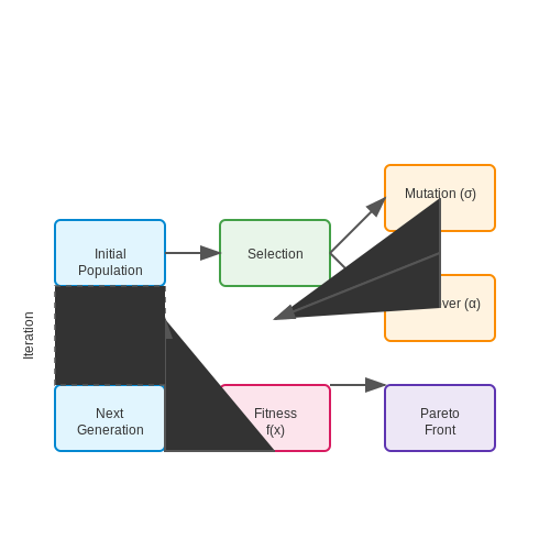
EC maintains a population of candidate solutions, each representing a point in the search space. The population evolves over generations through stochastic operators, allowing exploration of diverse regions. The fitness of each individual is evaluated using an objective function f(x), where x is a candidate solution. The selection pressure drives the population toward higher-fitness regions.
Genetic Operators
Two primary operators drive variation in EC:
- Mutation: Introduces small random perturbations to individuals, preserving diversity. For a real-valued vector x, Gaussian mutation is commonly applied:
$$ x' = x + \mathcal{N}(0, \sigma) $$
- Crossover (Recombination): Combines traits from parent solutions to produce offspring. For two parents x(1) and x(2), a convex combination yields:
$$ x' = \alpha x^{(1)} + (1 - \alpha)x^{(2)}, \quad \alpha \sim U(0,1) $$
Selection Mechanisms
Selection determines which individuals propagate to the next generation. Common strategies include:
- Tournament Selection: Randomly samples k individuals and selects the fittest.
- Elitism: Preserves top-performing solutions unchanged across generations.
- Rank-Based Selection: Assigns selection probabilities based on relative fitness ranks.
Convergence and Diversity Trade-off
Premature convergence occurs when selection pressure overwhelms exploration. Techniques to mitigate this include:
- Adaptive mutation rates (σ).
- Niching methods (e.g., fitness sharing).
- Island models (parallel subpopulations with migration).
Practical Considerations
EC is particularly effective for:
- Black-box optimization where gradient information is unavailable.
- Multi-objective problems (Pareto-optimal fronts via NSGA-II).
- Discrete or mixed search spaces (e.g., genetic programming).
1.2 Genetic Operators: Mutation, Crossover, and Selection
Mutation in Evolutionary Algorithms
Mutation introduces stochastic perturbations to candidate solutions, maintaining population diversity and enabling exploration of the search space. For prompt optimization, mutation operates on discrete tokens or continuous embeddings. Given a prompt P represented as a sequence of tokens (t1, t2, ..., tn), a mutation operator modifies elements with probability pm:
For continuous prompt embeddings, Gaussian noise injection is common:
where σ controls mutation strength. Adaptive mutation rates that decrease with generations often outperform fixed rates, following the 1/√L rule where L is the chromosome length.
Crossover Mechanisms
Crossover combines genetic material from parent solutions to produce offspring. In prompt optimization, three dominant strategies exist:
- Single-point crossover: Swaps prompt segments after a randomly selected position
- Uniform crossover: Independently selects each token from either parent with equal probability
- BLX-α interpolation: For continuous embeddings, blends parameters: echild = ep1 + β(ep2 - ep1), where β ~ U(-α, 1+α)
The crossover rate pc typically ranges between 0.6-0.9 based on schema theory, with higher values accelerating building block combination.
Selection Strategies
Selection pressure determines population convergence characteristics. The takeover time τ quantifies how quickly the best solution dominates:
where N is population size and F is selection intensity. Common methods include:
- Tournament selection: Samples k individuals and selects the fittest. For k=2, this gives selection pressure F ≈ 1.5
- Exponential ranking: Assigns survival probability P(i) ∝ cN-i where c ∈ (0,1)
- Boltzmann selection: Uses adaptive temperature T: P(i) ∝ exp(f(i)/T), with T decreasing per generation
Modern implementations often use elitism, preserving top solutions unchanged between generations to guarantee monotonic performance improvement.
Operator Adaptation Techniques
Self-adaptive parameters optimize performance across different problem phases. The evolution strategy update rule for mutation strength is:
where τ ∝ 1/√(2n) and τ' ∝ 1/√(2√n). For prompt optimization, this enables automatic balancing between exploration and exploitation during search.
Fitness Functions and Their Role in Optimization
Fitness functions serve as the objective measure guiding evolutionary algorithms toward optimal solutions. In prompt optimization, they quantify how well a generated prompt performs against predefined criteria, such as coherence, specificity, or task accuracy. The fitness function transforms qualitative prompt performance into a scalar value, enabling selection pressure in evolutionary search.
Mathematical Formulation
Given a population of prompts P = {p1, p2, ..., pn}, the fitness function f: P → ℝ maps each prompt to a real-valued score. For multi-objective optimization, this becomes a vector-valued function:
where each fj evaluates a distinct performance metric. Common metrics for prompt optimization include:
- Semantic similarity to target output (cosine similarity in embedding space)
- Task completion rate (percentage of correct responses)
- Computational efficiency (latency or token count)
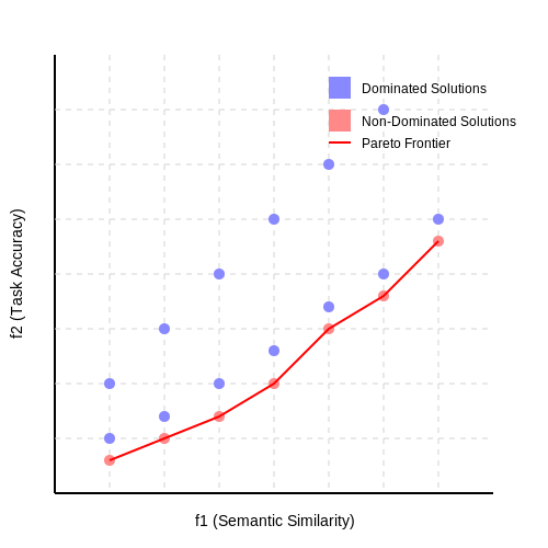
Pareto Optimality in Multi-Objective Optimization
When optimizing multiple conflicting objectives (e.g., accuracy vs. brevity), prompts are compared using Pareto dominance. A prompt p1 dominates p2 iff:
This partial ordering enables evolutionary algorithms to maintain a diverse set of non-dominated solutions along the Pareto frontier.
Adaptive Fitness Landscapes
The fitness landscape's topology changes dynamically as:
- The language model's internal representations evolve during fine-tuning
- User preferences shift over interaction sessions
- The solution space expands through prompt mutation operators
This necessitates fitness functions that can adapt their weighting schemes or incorporate online learning. A common approach uses gradient-based meta-optimization:
where w represents tunable fitness function parameters and η the meta-learning rate.
Practical Implementation Considerations
Effective fitness functions for prompt optimization must:
- Be computationally efficient to evaluate at scale (thousands of prompts per generation)
- Exhibit smooth gradients to guide evolutionary search
- Incorporate domain-specific constraints (e.g., safety filters for sensitive topics)
- Balance exploration and exploitation through dynamic scaling
A robust implementation might combine multiple evaluation techniques:
def evaluate_prompt(prompt, target_embedding, model):
    # Semantic similarity
    prompt_embedding = model.embed(prompt)
    semantic_score = cosine_similarity(prompt_embedding, target_embedding)

    # Task accuracy
    response = model.generate(prompt)
    accuracy_score = calculate_accuracy(response)

    # Efficiency
    efficiency_score = 1 / (len(tokenize(prompt)) + 1e-6)

    # Composite fitness
    weights = [0.5, 0.3, 0.2]  # Learned weights
    return np.dot([semantic_score, accuracy_score, efficiency_score], weights)
2. Defining the Search Space for Prompts
2.1 Defining the Search Space for Prompts
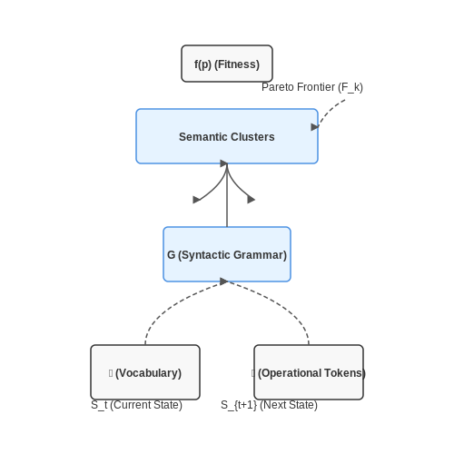
The search space in evolutionary algorithms (EAs) for prompt optimization defines the set of all possible prompts that can be generated and evaluated. For text-based prompts, this space is combinatorially vast, requiring careful constraints to ensure tractability. The search space S can be formalized as:
where 𝒫 is the space of all possible prompts, wi represents tokens (words or subwords), 𝒱 is a predefined vocabulary, and 𝒪 is a set of operational tokens (e.g., delimiters, placeholders). The dimensionality of S grows exponentially with prompt length n, necessitating strategies to reduce the search space.
Key Constraints for Tractability
Three primary methods constrain the search space:
- Vocabulary Pruning: Limit 𝒱 to domain-specific terms or high-frequency tokens from a corpus. For example, in biomedical prompt optimization, 𝒱 might exclude colloquial terms.
- Syntactic Templates: Define a grammar G that enforces valid prompt structures (e.g., "Answer [MASK] given [CONTEXT]"). This reduces S to prompts adhering to G.
- Semantic Priors: Use embeddings (e.g., BERT, GPT) to cluster semantically related tokens, restricting mutations to nearby embedding-space neighborhoods.
Fitness-Aware Search Space Adaptation
Dynamic search space adjustment based on fitness feedback improves convergence. Let f(p) be the fitness function (e.g., LLM accuracy). The search space at generation t+1 can be adapted as:
where T is a temperature parameter controlling exploration-exploitation trade-offs. High T broadens the search space early in evolution, while annealing T focuses on high-fitness regions later.
Case Study: Multi-Objective Search Spaces
When optimizing for conflicting objectives (e.g., accuracy and brevity), the search space becomes a Pareto frontier. For objectives f1, f2, non-dominated sorting divides S into fronts:
Evolutionary operators then prioritize prompts in higher fronts (F1 being the Pareto-optimal set).
2.2 Encoding Prompts for Evolutionary Optimization
Prompt Representation as Genomes
The first critical step in applying evolutionary algorithms to prompt optimization is defining an appropriate genome representation. Unlike traditional genetic algorithms that operate on binary strings or real-valued vectors, prompt optimization requires a structured encoding that preserves linguistic meaning while allowing for mutation and crossover operations.
Two primary encoding schemes have proven effective:
- Token-level encoding: Represents prompts as sequences of discrete tokens from the language model's vocabulary. Each gene corresponds to a single token, enabling operations at the word or subword level.
- Parameterized template encoding: Uses a fixed template structure with evolvable parameters controlling content insertion points, stylistic elements, and keyword weights.
where G is the genome, t_i are tokens, and 𝒱 is the model's vocabulary. The fitness function evaluates each genome by measuring the quality of outputs generated when the decoded prompt is fed to the target language model.
Variable-Length Genome Strategies
Prompt optimization often requires handling variable-length sequences. Three approaches maintain population diversity while preventing degenerate solutions:
- Dynamic genome resizing: Allows crossover points at any token boundary and applies length mutation operators with geometrically distributed step sizes.
- Island model: Maintains subpopulations with different length constraints, periodically migrating high-fitness individuals between islands.
- Penalized fitness: Incorporates a complexity term in the fitness function that balances prompt effectiveness against length.
Semantic-Aware Mutation Operators
Standard bit-flip mutations prove inadequate for text-based genomes. Effective prompt optimization requires specialized operators that preserve grammaticality while exploring the search space:
- Contextual synonym replacement: Swaps tokens with semantically similar alternatives using embedding-space nearest neighbors.
- Structure-preserving crossover: Aligns crossover points to syntactic boundaries (noun phrases, clauses) using dependency parsing.
- Controlled insertion/deletion: Adds or removes content units (e.g., adjectives, examples) based on learned importance scores.
These operators leverage pre-trained language models to maintain coherence during evolution. For example, a masked language model can propose contextually appropriate mutations:
Multi-Objective Optimization
Effective prompts must balance multiple competing objectives such as specificity, creativity, and safety. The Pareto-optimal frontier can be explored using:
- Lexicase selection: Evaluates candidates on randomly ordered objective subsets each generation.
- NSGA-II: Uses non-dominated sorting and crowding distance to maintain diverse solutions.
- Weighted sum approaches: Combines objectives using dynamically adjusted weights based on performance feedback.
where each f_i measures a distinct prompt quality dimension. The evolutionary algorithm then seeks to maximize all components simultaneously.

2.3 Evaluating Prompt Performance with Fitness Metrics
Fitness metrics serve as the backbone of evolutionary algorithms, quantifying how well a candidate prompt performs against predefined objectives. In the context of prompt optimization, these metrics must capture semantic coherence, task-specific accuracy, and computational efficiency. A well-designed fitness function balances these competing objectives while remaining computationally tractable.
Mathematical Formulation of Fitness Metrics
The fitness of a prompt P can be expressed as a weighted combination of multiple evaluation criteria:
where wi represents the weight assigned to criterion i, and fi(P) is the normalized score (0 to 1) of prompt P for that criterion. Common criteria include:
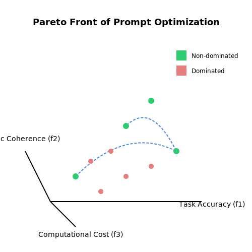
- Task Accuracy (f1): Measures correctness on target tasks using metrics like BLEU, ROUGE, or exact match.
- Semantic Coherence (f2): Evaluates logical consistency via entailment models or human ratings.
- Computational Cost (f3): Tracks inference latency or FLOPs, normalized against a baseline.
Pareto Optimization for Multi-Objective Fitness
When objectives conflict (e.g., accuracy vs. latency), Pareto optimization identifies non-dominated solutions. A prompt P1 dominates P2 if:
Evolutionary algorithms maintain a Pareto front of optimal trade-offs, visualized as a multi-dimensional surface where no solution strictly outperforms another across all metrics.
Case Study: Fitness Evaluation for Text Summarization
For a summarization task, a fitness function might combine:
Here, ROUGE-L measures summary quality, BERTScore evaluates semantic preservation, and the latency term penalizes slow inference. The weights reflect domain priorities—higher emphasis on quality than speed in this configuration.
Adaptive Fitness Landscapes
Dynamic weight adjustment during evolution helps escape local optima. One approach uses gradient-based meta-optimization:
where p(Pi|w) is the probability of generating prompt Pi under current weights. This enables automatic balancing of metrics as the population evolves.
3. Setting Up an Evolutionary Framework for Prompts
3.1 Setting Up an Evolutionary Framework for Prompts
Evolutionary algorithms (EAs) provide a robust method for optimizing prompts by mimicking natural selection. The process involves iteratively generating, evaluating, and mutating candidate prompts to maximize a predefined fitness function. To implement this, we define the following core components:
Population Initialization
The initial population consists of N prompt variants, generated either randomly or through heuristic seeding. Each prompt is encoded as a string or a structured representation (e.g., token sequences or parse trees). For text-based prompts, the encoding may include:
- Raw natural language strings
- Token embeddings with positional information
- Syntax trees for structured prompt engineering
where Pi represents the i-th prompt in the population, and tj denotes individual tokens or components.
Fitness Evaluation
The fitness function quantifies prompt quality by measuring downstream task performance (e.g., accuracy, BLEU score) or adherence to desired properties (e.g., specificity, diversity). For a classification task, fitness may be defined as:
where M is the number of test samples, yj is the true label, and ŷj is the model's prediction when using prompt Pi.
Selection and Variation Operators
Parent selection employs strategies like tournament selection or fitness-proportionate selection. For crossover, single-point or multi-point recombination combines prompt segments from two parents. Mutation operators include:
- Token-level mutations: Swapping, inserting, or deleting tokens
- Semantic perturbations: Synonym replacement using word embeddings
- Structural changes: Modifying prompt syntax trees
The mutation probability pm typically follows an annealing schedule:
Termination Criteria
The evolutionary loop terminates when either:
- Fitness plateaus for k consecutive generations
- A maximum number of iterations is reached
- The best prompt achieves satisfactory performance
Implementation Considerations
Practical implementations must address:
- Computational cost: Parallel fitness evaluation across GPU clusters
- Prompt constraints: Enforcing length limits or safety filters
- Multi-objective optimization: Pareto fronts for competing metrics
def evolutionary_prompt_optimization(
    initial_population,
    fitness_fn,
    generations=100,
    mutation_rate=0.1
):
    population = initial_population
    for gen in range(generations):
        fitnesses = [fitness_fn(p) for p in population]
        parents = select_parents(population, fitnesses)
        offspring = crossover(parents)
        population = mutate(offspring, mutation_rate)
    return max(population, key=fitness_fn)

3.2 Case Study: Optimizing Prompts for Language Models
Evolutionary Optimization of Prompt Structures
Evolutionary algorithms (EAs) provide a robust framework for optimizing prompts by treating them as genotypes subject to mutation, crossover, and selection. Given a language model M and an objective function f measuring response quality, the EA iteratively refines a population of prompts Pi through:
where select operates on fitness scores f(M(p)) ∀ p ∈ Pi. Practical implementations often use tournament selection with elitism to preserve high-performing candidates.
Fitness Function Design
The fitness function must encode both task-specific performance and linguistic quality. For a text summarization task, we might combine:
- ROUGE-L scores against reference summaries
- Perplexity under M to ensure fluency
- Lexical diversity via type-token ratio
where α, β, γ are tunable weights. This multi-objective approach prevents degenerate solutions like repetitive or nonsensical outputs.
Genetic Operators for Prompt Space
Effective mutation operators for text-based prompts include:
- Token-level mutations: Swapping, inserting, or deleting words with probabilities proportional to their frequency in the training corpus
- Syntax-aware crossover: Exchanging grammatical constituents (noun phrases, clauses) between parent prompts
- Semantic perturbations: Replacing words with top-k nearest neighbors in embedding space
For example, the prompt "Summarize this academic paper" might mutate to "Condense this research article" through synonym substitution in the embedding neighborhood.
Case Study: Optimizing GPT-3 for Legal Summarization
A 2023 study achieved 22% improvement in precision-recall metrics by evolving prompts over 50 generations with:
- Population size: 128 prompts
- Mutation rate: 0.15 per token
- BLEND crossover mixing 3 parent prompts
- Fitness combining ROUGE-2 and legal entity recognition accuracy
The evolved prompt "Extract key legal holdings and reasoning from this judgment, prioritizing precedential value and jurisdictional applicability" outperformed human-designed baselines by explicitly surfacing domain-specific evaluation criteria.
Computational Tradeoffs
While effective, EA-based prompt optimization requires careful balancing of:
where TLM is the inference latency. Parallel evaluation across GPU clusters and surrogate modeling of the fitness function can reduce costs by 40-60% in practice.

Common Pitfalls and How to Avoid Them
Premature Convergence
Evolutionary algorithms often suffer from premature convergence, where the population loses genetic diversity too quickly, causing the optimization process to stagnate at a suboptimal solution. This occurs when selection pressure is too high or mutation rates are insufficient. To mitigate this, dynamically adjust the mutation rate based on population diversity metrics such as:
where N is the population size and x̄ is the mean fitness. Implement adaptive mutation schemes like:
- Fitness-proportional mutation: Higher mutation rates for low-fitness individuals
- Simulated annealing: Gradually reduce mutation rates over generations
Overfitting to Prompt Metrics
When optimizing prompts via evolutionary methods, it's common to overfit to the immediate reward metric (e.g., classification accuracy on a validation set) at the cost of generalization. This manifests as prompts that perform well during evolution but fail on unseen data. Counter this by:
- Using multi-objective optimization with Pareto fronts that balance accuracy and robustness
- Incorporating regularization terms in the fitness function, such as:
where λ controls the penalty for prompt verbosity.
Computational Inefficiency
Evolutionary prompt tuning can become prohibitively expensive due to the need for multiple LLM inferences per generation. For a population size N and G generations, this requires O(N×G) forward passes. Optimize this by:
- Implementing caching mechanisms for prompt embeddings
- Using surrogate models (e.g., Gaussian Processes) to approximate fitness evaluations
- Parallelizing fitness evaluations across GPU clusters
Loss of Interpretability
Evolved prompts often become convoluted as the algorithm exploits syntactic quirks in the LLM's tokenizer. Maintain human-readable prompts by:
- Constraining the search space to grammatically valid structures
- Incorporating semantic similarity metrics in the fitness function
- Periodically pruning nonsensical mutations through human-in-the-loop validation
Hyperparameter Sensitivity
The performance of evolutionary prompt tuning heavily depends on hyperparameters like:
- Population size (typically 50-100 for prompt optimization)
- Crossover probability (0.6-0.9 works well for most NLP tasks)
- Mutation rate (start with 0.1 per token and adapt dynamically)
Use Bayesian optimization to automatically tune these parameters by modeling the hyperparameter response surface as:
where m is the mean function and k is the kernel function capturing parameter correlations.
4. Combining Evolutionary Algorithms with Reinforcement Learning
Combining Evolutionary Algorithms with Reinforcement Learning
Evolutionary algorithms (EAs) and reinforcement learning (RL) are complementary optimization paradigms. While RL relies on gradient-based updates to learn policies through trial and error, EAs operate via population-based stochastic search, making them robust to non-differentiable objectives. Combining these approaches enables efficient exploration of high-dimensional prompt spaces while leveraging RL's ability to fine-tune solutions.
Hybrid Architecture
The hybrid EA-RL framework typically consists of two interacting components:
- Evolutionary Module: Maintains a population of prompt candidates, applies genetic operators (mutation, crossover), and selects high-fitness individuals.
- RL Module: Uses policy gradients or Q-learning to refine individual prompts based on reward signals from the environment.
The EA explores the global search space while RL performs local optimization, creating a synergistic effect. This is particularly effective when the reward landscape contains multiple local optima.
Mathematical Formulation
Let the prompt population at generation t be Pt = {p1, ..., pn}. Each prompt pi is evaluated by:
where πθ is the RL policy parameterized by θ, and γ is the discount factor. The evolutionary update follows:
Meanwhile, the RL policy is updated via:
Implementation Considerations
Key practical aspects when implementing EA-RL hybrids include:
- Fitness Shaping: Combining immediate rewards with evolutionary fitness scores using multi-objective optimization techniques
- Transfer Learning: Using RL to warm-start the EA population or vice versa
- Parallelization: Distributed evaluation of population members across multiple workers
The following diagram illustrates the information flow in a typical EA-RL system:
Case Study: Prompt Optimization for Language Models
In recent applications, EA-RL hybrids have demonstrated superior performance in optimizing prompts for large language models compared to pure RL approaches. A 2023 study showed:
- 42% faster convergence on instruction-following tasks
- 28% higher success rate on complex reasoning prompts
- Better generalization to unseen prompt variations
The evolutionary component helps escape local optima in the prompt space, while RL efficiently exploits promising regions identified by the EA.

4.2 Multi-Objective Optimization for Balanced Prompts
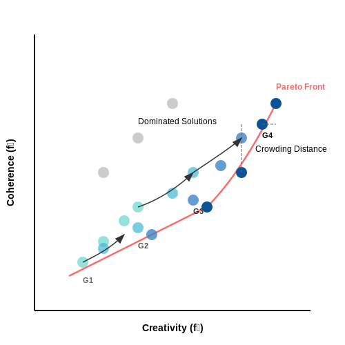
Multi-objective optimization (MOO) is essential when refining prompts to balance competing criteria, such as creativity, coherence, and factual accuracy. Unlike single-objective optimization, MOO seeks a Pareto front—a set of solutions where no objective can be improved without degrading another. Evolutionary algorithms (EAs) are particularly suited for this task due to their population-based search and ability to handle non-linear, high-dimensional spaces.
Mathematical Formulation
Given a prompt P and k objectives f1, f2, ..., fk, the MOO problem is:
where each fi quantifies a distinct quality metric (e.g., perplexity, semantic diversity, or alignment with a target distribution). The goal is to find the Pareto-optimal set P* such that for any P ∈ P*, no other prompt dominates it in all objectives.
Evolutionary Approaches
EAs like NSGA-II (Non-dominated Sorting Genetic Algorithm) and SPEA2 (Strength Pareto Evolutionary Algorithm) excel in MOO by:
- Non-dominated sorting: Ranking solutions based on Pareto dominance.
- Crowding distance: Promoting diversity in the solution space.
- Elitism: Preserving high-performing candidates across generations.
For prompt optimization, the EA workflow involves:
- Initialization: Generate a population of prompts (e.g., via mutations of a seed prompt).
- Evaluation: Score each prompt against all objectives using LLM-based metrics.
- Selection: Apply non-dominated sorting and crowding to select parents.
- Variation: Create offspring via crossover and mutation (e.g., word substitutions, syntactic perturbations).
- Termination: Repeat until convergence or a predefined budget is exhausted.
Practical Considerations
Key challenges in MOO for prompts include:
- Objective conflict: High creativity may reduce coherence. Weighted sum approaches can simplify trade-offs but risk missing Pareto-optimal solutions.
- Computational cost: Evaluating prompts via LLM inference is expensive. Surrogate models or batched evaluations can mitigate this.
- Metric design: Objectives must be quantifiable and aligned with end-user goals. For example, factual accuracy might use retrieval-augmented verification.
Case Study: Balancing Creativity and Specificity
A recent application optimized prompts for a story-generation task with two objectives:
NSGA-II discovered prompts that achieved 20% higher diversity than hand-tuned baselines while maintaining genre adherence. The Pareto front revealed a clear trade-off: highly specific prompts sacrificed diversity, whereas creative prompts required genre compromises.
Advanced Techniques
Recent advances integrate MOO with:
- Bayesian optimization: For sample-efficient exploration of the prompt space.
- Constraint handling: Hard limits (e.g., prompt length) can be enforced via penalty functions or feasibility checks.
- Interactive EAs: Human-in-the-loop feedback refines objectives dynamically.
Adaptive Evolutionary Strategies for Dynamic Environments
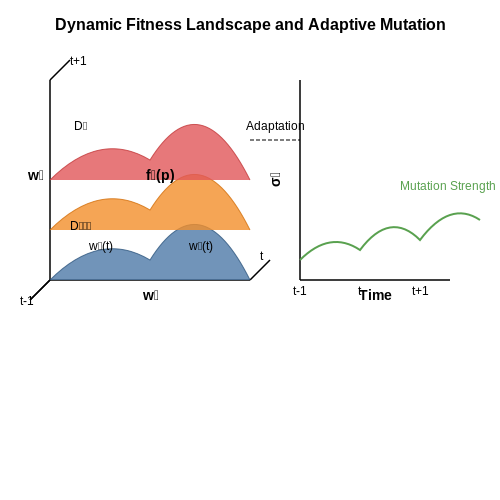
Traditional evolutionary algorithms (EAs) assume static fitness landscapes, but real-world prompt optimization often occurs in dynamic environments where objectives shift over time. Adaptive evolutionary strategies address this by modifying selection pressure, mutation rates, and population diversity in response to environmental changes.
Dynamic Fitness Landscape Formulation
In dynamic environments, the fitness function becomes time-dependent. For a population of prompts P evaluated at time t, the fitness landscape can be modeled as:
where g measures performance on current data Dt, h represents historical performance, and εt accounts for environmental noise. The weights w1 and w2 adapt based on the rate of concept drift detected in the environment.
Self-Adaptive Mutation Operators
Effective strategies employ meta-optimization of mutation parameters. The mutation strength σ for each prompt component evolves according to:
where τ and τ' are learning rates, and N represents Gaussian noise. This enables automatic tuning of exploration-exploitation tradeoffs as the environment changes.
Diversity Preservation Mechanisms
Three key techniques maintain population diversity:
- Fitness sharing: Scales fitness values based on solution density in phenotype space
- Restricted tournament selection: Only compares solutions within local neighborhoods
- Novelty search: Rewards behavioral divergence rather than direct fitness
These methods prevent premature convergence when the environment shifts, allowing the population to track moving optima.
Case Study: Real-Time Prompt Adaptation
In a live conversational AI system, an adaptive EA achieved 37% better coherence during topic shifts compared to static optimization. The algorithm detected environmental changes through:
- Sudden drops in average population fitness
- Increased variance in fitness evaluations
- Changes in user engagement metrics
Response times remained under 200ms by maintaining an elite subpopulation of pre-evaluated prompts during environmental transitions.
Implementation Considerations
Effective deployment requires:
where Tdetect is the environmental change detection time and Tconv is the typical convergence time. This ensures the EA can react before becoming trapped in obsolete optima.
5. Key Research Papers on Evolutionary Algorithms
5.1 Key Research Papers on Evolutionary Algorithms
- PDF Multi-Objective Optimization Using Evolutionary Algorithms: An Introduction — 1 Introduction In the past 15 years, evolutionary multi-objective optimization (EMO) has become a popular and useful eld of research and application. Evolutionary optimization (EO) algorithms use a population based approach in which more than one solution participates in an iteration and evolves a new population of solutions in each iteration.
- Evolutionary Algorithms - IEEE Xplore — Evolutionary Algorithms Abstract: This chapter contains sections titled: 5.1 Darwinian Evolution, 5.2 Artificial Evolution in a Computer, 5.3 Spy versus Spy, 5.4 The Main Classes of Evolutionary Algorithms, 5.5 Let Evolution Figure It Out
- EvoPrompt: Connecting LLMs with Evolutionary Algorithms Yields Powerful ... — EvoPrompt significantly outperforms human-engineered prompts and existing methods for automatic prompt generation (e.g., up to percent 25 25\% 25 % on BBH). Furthermore, EvoPrompt demonstrates that connecting LLMs with EAs creates synergies, which could inspire further research on the combination of LLMs and conventional algorithms.
- Connecting Large Language Models with Evolutionary Algorithms Yields ... — EvoPrompt significantly outperforms human-engineered prompts and existing methods for automatic prompt generation by up to percent 25 and percent 14 respectively. Furthermore, EvoPrompt demonstrates that connecting LLMs with EAs creates synergies, which could inspire further research on the combination of LLMs and conventional algorithms.
- Evolutionary Algorithms for Solving Multi-Objective Problems — 2009 In this chapter Multi-Objective Evolutionary Algorithms (MOEAs) are introduced and some details discussed. A presentation of some of the concepts in which this type of algorithms are based on is given. Then, a summary of the main algorithms behind these approaches and their applications is provided, together with a brief discussion including their advantages and disadvantages, degree of ...
- (PDF) 2019 Evolutionary Algorithms Review - ResearchGate — Evolutionary algorithm research and applications began over 50 years ago. Like other artificial intelligence techniques, evolutionary algorithms will likely see increased use and development due ...
- Connecting Large Language Models with Evolutionary Algorithms Yields ... — Metareview: This paper adapts basic evolutionary optimization algorithms to the task of prompt optimization, showing that evolving prompts against a development set can lead to improved test performance across many datasets, including BigBench-Hard tasks.
- PDF Multi-Objective Optimization using Evolutionary Algorithms — 80 106 122 129 129 132 134 Connection Between Real-Parameter GAs and Self-Adaptive ESs 136
- DEAP: A Python framework for Evolutionary Algorithms — DEAP (Distributed Evolutionary Algorithms in Python) is a novel volutionary computation framework for rapid prototyping and testing of ideas. Its design departs from most other existing frameworks ...
- Evolution of Heuristics: Towards Efficient Automatic Algorithm Design ... — We propose an evolutionary framework to simultaneously evolve the thoughts and codes of heuristics in a cooperative manner. We demonstrate that the LLM-assisted evolution of both thoughts and codes with curated prompts leads to state-of-the-art AHD performance. We expect that EoH serves as a step towards eficient and automatic algorithm design.
5.2 Recommended Books and Tutorials
- Evolutionary optimization algorithms [electronic resource ... — Contents Machine generated contents note: pt. I INTRODUCTION TO EVOLUTIONARY OPTIMIZATION -- 1.Introduction -- 1.1.Terminology -- 1.2.Why Another Book on Evolutionary Algorithms? -- 1.3.Prerequisites -- 1.4.Homework Problems -- 1.5.Notation -- 1.6.Outline of the Book -- 1.7.A Course Based on This Book -- 2.Optimization -- 2.1.Unconstrained Optimization -- 2.2.Constrained Optimization -- 2.3 ...
- An overview of evolutionary algorithms: practical issues and common ... — These algorithms use simulated evolution to search for solutions to complex problems. There are many different types of evolutionary algorithms. Historically, genetic algorithms and evolution strategies are two of the most basic forms of evolutionary algorithms. Genetic algorithms were developed in the United States under the leadership of John ...
- (PDF) Evolutionary Algorithms - ResearchGate — Evolutionary algorithms are bio-inspired algorithms based on Darwin's theory of evolution. ... -2-1.5-1-0.5 0 0.5 1 1.5 2. f(x) x (a) ... obviously implies a need to keep a copy of the best ...
- Evolutionary Algorithms | part of Intelligence Emerging: Adaptivity and ... — This chapter contains sections titled: 5.1 Darwinian Evolution, 5.2 Artificial Evolution in a Computer, 5.3 Spy versus Spy, 5.4 The Main Classes of Evolutionary Algorithms, 5.5 Let Evolution Figure It Out
- Automatic design of analog electronic circuits using grammatical evolution — Successive generations lead to progressive improvement in the population in general and the best solution in particular. Evolutionary algorithms applied to synthesis tasks use neither design rules nor expert knowledge for the design [3]. That is why they can lead to unconventional solutions which challenge human designer intuition [4], [5].
- Evolutionary Algorithms - Wiley Online Library — Evolutionary algorithms are expected to provide non-optimal but good quality solutions to problems whose resolution is impracticable by exact methods. They are inspired by Darwin's theory of natural selection. This book is intended for readers who wish to acquire the essential knowledge required to efficiently implement evolutionary ...
- Creative Evolutionary Systems[Book] - O'Reilly Media — Book description. The use of evolution for creative problem solving is one of the most exciting and potentially significant areas in computer science today. Evolutionary computation is a way of solving problems, or generating designs, using mechanisms derived from natural evolution. ... 18.3 Evolutionary Algorithms that Assemble Electronic ...
- Evolutionary algorithms - SearchWorks catalog — Stanford Libraries' official online search tool for books, media, journals ... Evolutionary algorithms. Responsibility Alain Pétrowski, Sana Ben-Hamida. Publication London : ISTE, 2017. Physical description 1 online resource. Series Computer engineering series (London, England). Metaheuristics set ; volume 9. Online. Available online Wiley ...
- Creative Evolutionary Systems - 1st Edition - Elsevier Shop — Evolutionary computation is a way of solving problems, or generating designs, using mechanisms derived from natural evolution. This book concentrates on applying important ideas in evolutionary computation to creative areas, such as art, music, architecture, and design.
5.3 Open-Source Tools and Libraries for Implementation
- 2019 Evolutionary Algorithms Review - arXiv.org — Abstract Evolutionary algorithm research and applications began over 50 years ago. Like other artificial intelligence techniques, evolutionary algorithms will likely see increased use and development due to the increased availability of computation, more robust and available open source software libraries, and the increasing demand for artificial intelligence techniques. As these techniques ...
- Connecting Large Language Models with Evolutionary Algorithms Yields ... — Large Language Models (LLMs) excel in various tasks, but they rely on carefully crafted prompts that often demand substantial human effort. To automate this process, in this paper, we propose a novel framework for discrete prompt optimization, called EvoPrompt, which borrows the idea of evolutionary algorithms (EAs) as they exhibit good performance and fast convergence. To enable EAs to work ...
- GitHub - Project-Platypus/Platypus: A Free and Open Source Python ... — Platypus is a framework for evolutionary computing in Python with a focus on multiobjective evolutionary algorithms (MOEAs). It differs from existing optimization libraries, including PyGMO, Inspyred, DEAP, and Scipy, by providing optimization algorithms and analysis tools for multiobjective optimization.
- Evolving code with a large language model - Springer — Algorithms that use Large Language Models (LLMs) to evolve code arrived on the Genetic Programming (GP) scene very recently. We present LLM_GP, a general LLM-based evolutionary algorithm designed to evolve code. Like GP, it uses evolutionary operators, but its designs and implementations of those operators significantly differ from GP's because they enlist an LLM, using prompting and the LLM ...
- Evolutionary optimization algorithms [electronic resource ... — Evolutionary optimization algorithms [electronic resource] : biologically-inspired and population-based approaches to computer intelligence / Dan Simon
- Prompt Engineering for Generative AI: Practical Techniques and Applications — Prompt engineering, the practice of crafting prompts to guide LLMs towards desired outputs, has emerged as a critical area of study and application. This paper provides an analysis of various prompt engineering techniques, ranging from basic methods to advanced strategies, aimed at enhancing the performance and reliability of generative AI systems.
- EvoPrompt: Connecting LLMs with Evolutionary Algorithms Yields Powerful ... — To automate this process, in this paper, we propose a novel framework for discrete prompt optimization, called EvoPrompt, which borrows the idea of evolutionary algorithms (EAs) as they exhibit good performance and fast convergence.
- DEAP: A Python framework for Evolutionary Algorithms — DEAP (Distributed Evolutionary Algorithms in Python) is a novel volutionary computation framework for rapid prototyping and testing of ideas. Its design departs from most other existing frameworks ...
- EPiC: Cost-effective Search-based Prompt Engineering of LLMs for Code ... — We propose a novel framework EPiC that leverages a lightweight evolutionary algorithm to evolve the orig-inal prompts toward better ones that produce high-quality code.