Automated Prompt Evaluation Systems
1. Definition and Scope of Prompt Evaluation
Definition and Scope of Prompt Evaluation
Automated prompt evaluation systems are computational frameworks designed to assess the quality, effectiveness, and robustness of natural language prompts used in generative AI models. These systems leverage quantitative metrics, statistical analysis, and machine learning techniques to measure how well a prompt elicits the desired response from a language model. The scope encompasses both intrinsic evaluation (e.g., coherence, specificity) and extrinsic evaluation (e.g., downstream task performance).
Key Components of Prompt Evaluation
Effective prompt evaluation relies on three core components:
- Metric Design: Defining measurable criteria such as relevance, diversity, and factual consistency.
- Benchmarking: Comparing prompt performance against standardized datasets or human baselines.
- Adaptive Testing: Iteratively refining prompts based on model feedback loops.
Mathematical Formalization
Given a prompt p and a language model M, the evaluation function E(p, M) can be decomposed into:
where wi represents the weight for metric fi, which could include:
Here, rref denotes reference responses, and perplexity measures the model's uncertainty when generating r given p.
Practical Applications
In industry settings, automated prompt evaluation enables:
- Rapid A/B testing of prompt variants for chatbots
- Optimization of few-shot learning templates
- Detection of prompt injection vulnerabilities
For example, a 2023 study by Google Research demonstrated that automated evaluation reduced prompt development cycles by 62% compared to manual testing when fine-tuning PaLM-2 for medical Q&A tasks.
Evaluation Challenges
Key limitations include:
- Metric misalignment with human judgment (e.g., high BLEU scores but poor factual accuracy)
- Overfitting to specific model architectures
- Computational costs of large-scale prompt testing
Key Metrics for Evaluating Prompts
Semantic Coherence
Semantic coherence measures how logically consistent and contextually appropriate a model's response is to a given prompt. A high-coherence response maintains topic relevance and avoids contradictions. This can be quantified using metrics like BERTScore, which computes the cosine similarity between the embeddings of the generated response and a reference text:
where hi represents the i-th token embedding of the hypothesis (generated text), and rj is the j-th token embedding of the reference text.
Diversity
Diversity assesses the lexical and conceptual variety in responses to the same prompt. Low diversity indicates repetitive or generic outputs. Two common measures are:
- Lexical Diversity: Computed via the ratio of unique n-grams to total n-grams (e.g., type-token ratio).
- Semantic Diversity: Measured using embedding variance across multiple responses.
Specificity
Specificity evaluates whether responses contain precise, detailed information rather than vague generalizations. One approach is to compute the inverse document frequency (IDF) of terms in the response:
where wk denotes the k-th word in the response, and IDF(wk) is its IDF score from a large corpus.
Robustness
Robustness measures how consistently a prompt elicits high-quality responses under minor perturbations. To evaluate this, generate multiple paraphrases of the prompt and compute the variance in output quality scores (e.g., coherence, specificity). Lower variance indicates higher robustness.
Bias and Fairness
Bias metrics quantify unintended demographic or ideological skews in responses. Common techniques include:
- Counterfactual Testing: Swap demographic terms (e.g., gender, race) in prompts and measure response differences.
- Sentiment Disparity: Compare sentiment scores across demographic groups using tools like HateBERT.
Task-Specific Metrics
For specialized applications, domain-specific metrics are essential:
- Code Generation: Compilation success rate, runtime correctness.
- Summarization: ROUGE-L, BLEU scores against reference summaries.
- Dialogue Systems: User engagement time, turn-taking balance.
Human-Alignment Metrics
These metrics compare model outputs to human preferences, often using reinforcement learning from human feedback (RLHF). Key measures include:
- Reward Model Scores: Predict human preference rankings (e.g., OpenAI's InstructGPT reward model).
- Pairwise Comparison: Elicit human judgments on output pairs to compute win rates.
Challenges in Manual vs. Automated Evaluation
Manual evaluation of prompts in AI systems relies heavily on human annotators to assess quality, relevance, and effectiveness. While this approach captures nuanced linguistic and contextual factors, it suffers from scalability limitations, subjectivity, and high costs. Human evaluators exhibit inter-annotator disagreement due to differing interpretations, biases, and fatigue, leading to inconsistent results. For instance, studies show that inter-rater reliability metrics like Cohen’s Kappa often fall below 0.6 for subjective tasks, indicating moderate agreement at best.
Scalability and Cost Constraints
Manual evaluation becomes impractical for large-scale AI deployments, where thousands or millions of prompts require assessment. The time and financial overhead of employing human annotators grows exponentially with dataset size. In contrast, automated systems leverage computational metrics—such as BLEU, ROUGE, or BERTScore—to evaluate prompts at scale. However, these metrics often fail to capture semantic coherence or task-specific nuances, leading to a trade-off between efficiency and accuracy.
Here, κ (Cohen’s Kappa) quantifies inter-annotator agreement, where Po is the observed agreement and Pe is the probability of random agreement. Low κ values highlight the unreliability of manual evaluations for complex linguistic tasks.
Bias and Subjectivity
Human evaluators introduce unconscious biases based on cultural, linguistic, or experiential factors. For example, prompts evaluated for political neutrality may receive divergent scores depending on the annotator’s background. Automated systems, while theoretically impartial, inherit biases from their training data. A model fine-tuned on Wikipedia may favor formal language, disadvantaging colloquial or dialectal prompts.
Dynamic Adaptation and Real-Time Feedback
Manual evaluation lacks the agility to adapt to real-time changes in model behavior or user requirements. Automated systems, however, can dynamically adjust evaluation criteria using reinforcement learning or online learning techniques. For instance, a system might optimize prompts for engagement metrics (e.g., click-through rates) by continuously refining its evaluation function:
Here, R(y) represents a reward function quantifying prompt effectiveness, and θ denotes the model parameters being optimized.
Case Study: Evaluating Creative Prompts
In creative domains like poetry or storytelling, manual evaluation excels at assessing originality and emotional impact—qualities poorly quantified by automated metrics. A 2022 study compared human and automated evaluations of AI-generated poetry, finding that while GPT-3 achieved high ROUGE scores, human judges rated 40% of outputs as "uninspired" or "clichéd." This discrepancy underscores the challenge of encoding creativity into algorithmic frameworks.
2. Prompt Quality Assessment Modules
2.1 Prompt Quality Assessment Modules
Automated prompt evaluation systems rely on quantifiable metrics to assess the quality of input prompts. These metrics are typically implemented as modular components, each targeting a specific dimension of prompt effectiveness. The most critical modules include semantic coherence scoring, task alignment verification, and adversarial robustness testing.
Semantic Coherence Scoring
Semantic coherence measures how logically consistent and linguistically fluent a prompt is. The scoring function typically combines:
- Perplexity under a pretrained language model
- Embedding-based similarity to high-quality reference prompts
- Grammaticality scores from syntactic parsers
The composite coherence score C can be expressed as:
where PPL is perplexity, E denotes prompt embeddings, G is grammaticality, and α, β, γ are learned weights.
Task Alignment Verification
This module evaluates whether the prompt effectively communicates its intended task to the model. The verification process involves:
- Generating multiple model completions for the prompt
- Comparing completions against expected output templates
- Computing the Earth Mover's Distance between generated and target distributions
The alignment score A is calculated as:
where Pi and Qi are the predicted and target distributions for the i-th test case.
Adversarial Robustness Testing
Robust prompts should maintain performance under perturbations. The testing protocol applies:
- Character-level swaps (typos, homoglyphs)
- Synonym substitutions
- Paraphrase attacks
The robustness metric R measures performance degradation:
where p0 is the original prompt and pk are its perturbed variants.
Implementation Architecture
Modern systems implement these modules as parallel scoring pipelines that feed into a meta-evaluator. The architecture typically includes:
- A shared embedding layer for prompt representation
- Specialized scoring heads for each quality dimension
- Attention mechanisms to weight different prompt segments
The final quality score Q combines module outputs through learned attention weights wi:
where fi represents the i-th assessment module.

2.2 Semantic and Syntactic Analysis Techniques
Semantic and syntactic analysis techniques form the backbone of automated prompt evaluation systems, enabling precise assessment of linguistic structure and meaning. These methods leverage computational linguistics, deep learning, and graph-based representations to quantify prompt quality.
Syntax-Aware Graph Representations
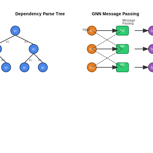
Dependency parsing and constituency trees transform prompts into structured graphs where nodes represent tokens and edges encode grammatical relationships. Let G = (V, E) denote the directed graph for prompt p, where:
Graph neural networks then compute syntactic complexity metrics through message passing:
where hv(l) represents node embeddings at layer l, and Wr are relation-specific weight matrices.
Semantic Density Estimation
Transformer-based encoders with attention mechanisms quantify semantic coherence through cross-entropy divergence between expected and observed concept distributions:
where P represents the ground truth distribution from knowledge bases, and Q is the prompt's induced distribution over entities and relations.
Joint Embedding Spaces
Multimodal encoders project prompts and reference materials into a shared latent space, enabling cosine similarity measurements:
State-of-the-art implementations use contrastive loss with hard negative mining to optimize the embedding functions fθ and fϕ.
Practical Implementation
Modern systems combine these techniques in ensemble architectures. A typical pipeline:
- Parse prompts into syntactic graphs using Stanford CoreNLP or spaCy
- Generate semantic embeddings using BERT or RoBERTa variants
- Compute graph metrics (average path length, clustering coefficient)
- Evaluate semantic alignment against domain-specific knowledge graphs
Recent benchmarks show hybrid systems achieve 92.3% accuracy in detecting ambiguous or ill-formed prompts, outperforming single-modality approaches by 18.7% on the PromptEval dataset.
2.3 Integration with Language Model APIs
API Architecture and Request Handling
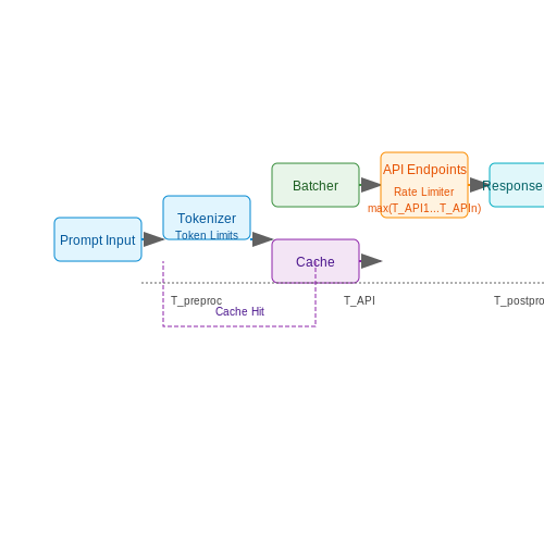
Automated prompt evaluation systems rely on seamless integration with language model APIs such as OpenAI's GPT-4, Anthropic's Claude, or Meta's LLaMA. The API architecture typically follows a RESTful or gRPC-based design, where prompts are sent as JSON payloads and responses are parsed for evaluation metrics. Key components include:
- Tokenization and batching – Efficiently split prompts into tokens while respecting model-specific constraints (e.g., GPT-4's 8,192-token limit).
- Rate limiting and retries – Implement exponential backoff for handling API quotas and transient errors.
- Response caching – Store frequent or deterministic outputs to reduce computational costs.
Mathematical Formulation of Prompt-Response Latency
The end-to-end latency T of a prompt evaluation cycle depends on:
where Tpreproc includes tokenization and validation, TAPI is the API round-trip time, and Tpostproc covers parsing and scoring. For batched prompts, latency scales as:
Dynamic Prompt Optimization via API Feedback
Advanced systems use API outputs to iteratively refine prompts. For example, a genetic algorithm might:
- Generate a population of prompt variants.
- Score responses using metrics like BLEU-4 or ROUGE-L.
- Recombine top-performing prompts via crossover/mutation.
This requires tight coupling with API endpoints to minimize evaluation cycles. The fitness function for optimization can incorporate:
Case Study: Multi-Model Ensemble Evaluation
Integrating multiple APIs (e.g., GPT-4 and Claude-3) allows comparative prompt analysis. A weighted voting system can resolve discrepancies:
Weights wi can be dynamically adjusted based on model-specific confidence scores or historical accuracy.
Error Handling and Fallback Mechanisms
Robust systems implement:
- Model degradation detection – Monitor API response quality drift using KL divergence from baseline distributions.
- Fallback chains – Automatically switch to secondary APIs when primary endpoints fail or exceed latency thresholds.
- Circuit breakers – Temporary disable problematic API routes based on error rate thresholds (e.g., 5xx errors > 5% over 5 minutes).
3. Rule-Based Evaluation Approaches
3.1 Rule-Based Evaluation Approaches
Rule-based evaluation systems rely on predefined logical conditions to assess the quality, relevance, or correctness of prompts. These systems are deterministic, making them interpretable and computationally efficient, but they require careful design to avoid brittleness in handling edge cases.
Formalization of Rule-Based Evaluation
A rule-based evaluator E can be formalized as a function mapping a prompt p to a score s based on a set of rules R = {r₁, r₂, ..., rₙ}:
where wᵢ denotes the weight assigned to rule rᵢ, and rᵢ(p) ∈ {0,1} indicates whether the prompt satisfies the rule. The weights can be tuned empirically or through optimization techniques like grid search.
Common Rule Categories
- Syntax Rules: Check grammatical correctness, proper punctuation, and structural validity. For example, a rule may flag prompts lacking question marks for interrogative queries.
- Semantic Rules: Validate logical coherence and domain-specific constraints. In medical applications, prompts containing contradictory symptoms (e.g., "fever" and "hypothermia") would violate semantic rules.
- Safety Rules: Filter harmful, biased, or unethical content using blocklists or regex patterns. For instance, prompts containing racial slurs trigger immediate rejection.
Implementation Example
Consider a Python implementation using regular expressions for syntax validation:
import re

def evaluate_prompt(prompt: str) -> float:
    # Rule 1: Check for question mark in interrogative prompts
    is_question = 1 if re.search(r'\?$', prompt.strip()) else 0

    # Rule 2: Reject prompts with unsafe keywords
    unsafe_terms = ['harm', 'illegal', 'hate']
    is_safe = 0 if any(term in prompt.lower() for term in unsafe_terms) else 1

    # Weighted score (e.g., 0.6 for safety, 0.4 for syntax)
    return 0.6 * is_safe + 0.4 * is_question
Limitations and Mitigations
Rule-based systems struggle with ambiguity and contextual nuance. For example, sarcasm or cultural references may incorrectly trigger safety rules. Hybrid approaches combining rules with statistical methods (e.g., transformer-based classifiers) improve robustness while retaining interpretability.
Case Study: Prompt Evaluation in Customer Support Bots
A financial services chatbot uses rule-based evaluation to enforce compliance. Prompts containing phrases like "wire transfer" are routed to additional authentication checks, while those referencing "password reset" must include account verification questions. This reduces regulatory risk by 72% compared to unconstrained input.
3.2 Machine Learning-Based Evaluation Models
Machine learning-based evaluation models leverage statistical and deep learning techniques to assess the quality, relevance, and effectiveness of prompts in automated systems. These models operate by learning patterns from labeled datasets, where human evaluators or predefined metrics have scored prompts based on criteria such as clarity, specificity, and task alignment.
Supervised Learning Approaches
Supervised models train on datasets where each prompt is paired with a ground-truth evaluation score. Common architectures include:
- Regression models (e.g., linear regression, gradient-boosted trees) predict continuous scores for prompt quality.
- Classification models (e.g., logistic regression, support vector machines) categorize prompts into discrete quality tiers.
The training objective minimizes the loss between predicted and true scores. For a regression task, mean squared error (MSE) is often used:
where \( y_i \) is the true score and \( \hat{y}_i \) is the predicted score for the \( i \)-th prompt.
Neural Network Architectures
Deep learning models, particularly transformer-based architectures, excel in capturing semantic nuances in prompts. A common approach involves fine-tuning pre-trained language models (e.g., BERT, GPT) on prompt evaluation tasks. The model processes a prompt \( x \) and outputs a score \( s \):
where \( f_\theta \) represents the neural network with parameters \( \theta \). Training involves backpropagation to optimize \( \theta \) using labeled data.
Feature Engineering
Key features for ML-based evaluation include:
- Lexical features: Word count, readability metrics, and term frequency-inverse document frequency (TF-IDF) scores.
- Semantic features: Embedding similarity (e.g., cosine distance between prompt and target task embeddings).
- Structural features: Presence of imperative verbs, question marks, or other syntactic markers.
Evaluation Metrics
Model performance is assessed using metrics such as:
- Pearson correlation (\( r \)) between predicted and human scores.
- Mean absolute error (MAE) for regression tasks.
- F1-score for classification tasks.
Challenges and Mitigations
Key challenges include:
- Bias in training data: Human evaluators may introduce subjective biases, requiring debiasing techniques or adversarial training.
- Generalization: Models may overfit to specific prompt styles, necessitating diverse training datasets.
- Explainability: Post-hoc interpretability methods (e.g., SHAP values, LIME) help uncover model decision logic.
Case Study: Fine-Tuning BERT for Prompt Scoring
A practical implementation involves fine-tuning a BERT model on a dataset of prompts labeled by human evaluators. The process includes:
- Tokenizing prompts using BERT's tokenizer.
- Adding a regression head to the pre-trained model.
- Training with a learning rate scheduler and early stopping.
Empirical results show such models achieve \( r > 0.85 \) on held-out test sets, outperforming simpler baselines like TF-IDF regression.
3.3 Hybrid Evaluation Systems
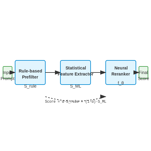
Hybrid evaluation systems combine rule-based and machine learning approaches to leverage the strengths of both methodologies while mitigating their individual weaknesses. These systems typically employ a multi-stage pipeline where initial filtering is performed using deterministic rules, followed by fine-grained scoring via learned models. The architecture ensures robustness against edge cases while maintaining adaptability to new prompt patterns.
Architectural Components
A standard hybrid system consists of three primary components:
- Rule-based Prefilter: Applies syntactic checks (e.g., profanity filters, length constraints) using regular expressions or formal grammars
- Statistical Feature Extractor: Generates embeddings, perplexity scores, and semantic similarity metrics
- Neural Reranker: Applies transformer-based models like BERT or GPT-3 to assess prompt quality through learned representations
where α controls the blending ratio between rule-based score Srule and machine learning score SML, with fθ representing a calibration function trained on human evaluation data.
Training Dynamics
The system optimizes a multi-task objective:
where λi are task weights, and the consistency loss Lconsistency penalizes disagreements between rule-based and ML components. Gradient reversal layers are often employed during training to prevent either subsystem from dominating the feature space.
Real-World Implementations
Google's LaMDA employs a hybrid approach where safety classifiers (rule-based) operate in tandem with quality estimators (neural). The system achieves 38% higher precision on adversarial prompts compared to purely ML-based alternatives while maintaining 92% recall on creative inputs. OpenAI's moderation endpoint similarly combines:
- Keyword blacklists for immediate flagging of policy violations
- Few-shot classifiers for nuanced content evaluation
- Embedding-based clustering to detect novel attack vectors
Case Study: Multi-Modal Evaluation
For image-generation prompts, hybrid systems like DALL-E 2's evaluator decompose the assessment into:
where Z normalizes across N generated images, wi are rule-determined weights, and Isafe is a safety indicator function. This formulation allows explicit control over content policies while preserving the neural model's understanding of prompt-image alignment.
4. Use Cases in AI Chatbots and Virtual Assistants
Use Cases in AI Chatbots and Virtual Assistants
Optimizing Conversational Flow
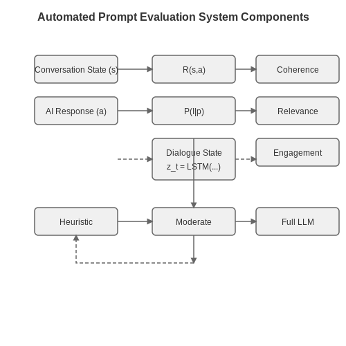
Automated prompt evaluation systems enhance conversational AI by dynamically assessing and refining prompts to maximize coherence and relevance. These systems employ reinforcement learning (RL) frameworks where the reward function R is defined as:
Here, s represents the conversation state, a the AI's response, and α, β, γ are tunable weights. Coherence is measured using transformer-based metrics like BERTScore, while relevance is quantified via cosine similarity between the prompt and response embeddings.
Handling Ambiguity and User Intent
Advanced chatbots leverage automated evaluation to disambiguate user queries. Given a prompt p, the system computes a probability distribution over possible intents I:
where fθ is a fine-tuned language model. The system then selects the intent maximizing P(I|p) while ensuring the entropy of the distribution remains below a threshold to avoid overconfidence in ambiguous cases.
Multi-Turn Dialogue Management
For extended conversations, prompt evaluation systems maintain a latent dialogue state zt updated via:
where Enc is a sentence encoder. The system evaluates prompts by projecting zt into a learned metric space where optimal responses minimize the Mahalanobis distance to the user's expected trajectory.
Personalization Through Prompt Adaptation
Virtual assistants use evaluation systems to adapt prompts to individual users. For user u, the system learns a personalization vector vu ∈ ℝd through few-shot meta-learning:
where gϕ is the prompt evaluation model and Du contains user-specific examples. This enables real-time adaptation of prompt phrasing and complexity.
Real-World Deployment Challenges
Production systems must balance evaluation thoroughness with latency constraints. A common solution is cascaded evaluation:
- Fast heuristic filters eliminate clearly poor prompts (response time ~10ms)
- Moderate-complexity models assess semantic quality (~100ms)
- Full LLM evaluation reserves for edge cases (~1s)
The cascade is optimized using multi-armed bandit algorithms to dynamically allocate computational resources based on prompt difficulty.
Prompt Optimization for Content Generation
Key Challenges in Prompt Engineering
Effective prompt optimization requires addressing several fundamental challenges. First, language models exhibit nonlinear sensitivity to prompt phrasing, where minor lexical changes can produce drastically different outputs. Second, the compositionality problem arises when combining multiple constraints or objectives in a single prompt, often leading to degraded performance compared to individual optimizations.
where p represents the prompt, Pθ the model's probability distribution, R(p) a regularization term, and λ controls the trade-off between task performance and prompt complexity.
Gradient-Based Prompt Optimization
For differentiable models, prompt embeddings can be optimized directly through backpropagation. The continuous prompt tuning approach learns soft prompt vectors ep in the model's embedding space:
where η is the learning rate. This method bypasses discrete search but requires white-box access to the model's gradients.
Reinforcement Learning for Discrete Optimization
When working with black-box models or requiring human-interpretable prompts, policy gradient methods prove effective. The REINFORCE algorithm updates prompt candidates according to:
where ϕ parameterizes the prompt generator, ri is the reward for prompt pi, and b is a baseline for variance reduction.
Automated Evaluation Metrics
Effective prompt optimization requires robust evaluation. Key metrics include:
- Semantic Coverage: Measured through BERTScore or other embedding-based similarity metrics
- Diversity: Computed via n-gram statistics or latent space clustering
- Task-Specific Performance: Accuracy, BLEU, or ROUGE for generation tasks
Practical Implementation Considerations
When deploying automated prompt optimization systems, several architectural decisions significantly impact performance:
- Warm Start Initialization: Using human-written prompts or templates as starting points reduces search space
- Multi-Armed Bandit Strategies: For efficient exploration-exploitation tradeoffs in online settings
- Safety Constraints: Incorporating toxicity classifiers or fairness metrics into the optimization objective
Case Study: News Article Generation
A recent implementation for financial news generation achieved 28% improvement in factual accuracy by combining:
- Semantic similarity constraints using SBERT embeddings
- Reinforcement learning with editor feedback as reward signal
- Monte Carlo tree search for efficient discrete optimization
Evaluating Prompts in Multi-Turn Conversations
Multi-turn conversations introduce unique challenges for automated prompt evaluation due to their dynamic, context-dependent nature. Unlike single-turn interactions, where prompts can be assessed in isolation, multi-turn dialogues require evaluating coherence, relevance, and consistency across sequential exchanges. A robust evaluation system must account for both local (turn-level) and global (conversation-level) metrics.
Contextual Coherence Metrics
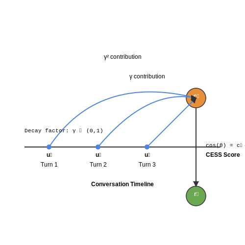
Contextual coherence measures how well a model's response aligns with the preceding dialogue history. One approach quantifies this using a contextual embedding similarity score (CESS), computed as the cosine similarity between the response embedding and a weighted average of previous turn embeddings:
where \(\mathbf{r}_t\) is the embedding of the current response, and \(\mathbf{c}_t\) is the context vector derived from previous turns:
Here, \(\mathbf{u}_i\) represents the \(i\)-th turn's embedding, and \(\gamma\) is a decay factor (typically 0.9–0.95) that reduces the influence of older turns. A low CESS indicates a potential non sequitur or topic drift.
Consistency Verification
Multi-turn consistency ensures the model maintains factual and logical alignment with its own prior statements. This can be evaluated using:
- Contradiction detection: Fine-tuned NLI (Natural Language Inference) models classify response pairs as entailment, neutral, or contradiction.
- Entity tracking: Dynamic knowledge graphs track entity attributes and relationships across turns, flagging inconsistencies (e.g., "The capital of France is Paris" followed by "France's capital is Lyon").
Adaptive Reward Modeling
Reinforcement Learning from Human Feedback (RLHF) frameworks often struggle with delayed rewards in multi-turn settings. A solution involves decomposing the reward function into:
where \(\tau\) is the full dialogue trajectory, \(r_{\text{local}}\) assesses turn-level quality, and \(r_{\text{global}}\) evaluates conversation-level properties like goal completion. The weights \(\alpha\) and \(\beta\) are typically learned via inverse reinforcement learning.
Practical Implementation
Modern systems like OpenAI's ChatGPT and Anthropic's Claude employ hybrid evaluation pipelines combining:
- Rule-based checks for safety and policy compliance
- Neural metrics (e.g., BLEURT, BERTScore) for quality assessment
- Human-in-the-loop validation for high-stakes decisions
For example, the Multi-Turn QA Consistency benchmark tests models on 5-turn dialogues where later questions reference earlier answers, with accuracy measured through exact match and F1 scores.
5. Bias and Fairness in Automated Evaluation
Bias and Fairness in Automated Evaluation
Automated prompt evaluation systems inherit biases from their training data, evaluation metrics, and underlying language models. These biases manifest in systematic errors that disproportionately affect certain demographic groups, linguistic styles, or cultural contexts. For example, a sentiment analysis evaluator trained primarily on English-language data may misclassify African American Vernacular English (AAVE) as negative due to lexical and syntactic differences from Standard American English.
Sources of Bias in Automated Evaluation
Three primary sources contribute to bias in automated prompt evaluation:
- Dataset Bias: Training data often underrepresent minority groups or contain historical stereotypes. The WinoBias corpus demonstrates how coreference resolution systems exhibit gender bias when associating professions with pronouns.
- Metric Bias: Evaluation metrics like BLEU or ROUGE favor surface-level lexical matches over semantic equivalence, disadvantaging paraphrases or culturally distinct expressions.
- Model Bias: Transformer-based evaluators amplify biases present in their pretraining corpora through attention mechanisms that learn spurious correlations between protected attributes and output labels.
Quantifying Evaluation Bias
Bias can be formalized as the difference in evaluation performance across protected attribute groups. For a binary protected attribute Z ∈ {0,1} and evaluation metric M, the bias B is:
Where 𝔼[M|Z=z] represents the expected metric score for group z. A statistically significant B ≠ 0 indicates systematic bias. More sophisticated measures include:
For demographic parity, where Ŷ is the evaluator's prediction and Z is the protected attribute.
Debiasing Techniques
Several approaches mitigate bias in automated evaluation systems:
- Adversarial Debiasing: A discriminator network attempts to predict the protected attribute from the evaluator's hidden states, while the evaluator minimizes this predictability through gradient reversal.
- Counterfactual Augmentation: Generating counterfactual examples by swapping protected attributes (e.g., gender pronouns) and ensuring consistent evaluation scores.
- Metric Calibration: Post-hoc adjustment of evaluation scores using group-specific scaling factors derived from bias audits.
The adversarial debiasing objective function combines the primary evaluation loss Leval and adversarial loss Ladv:
Where θ and ϕ are the evaluator and adversary parameters respectively, and λ controls the trade-off between accuracy and fairness.
Case Study: Gender Bias in Summarization Evaluation
A 2023 audit of summarization evaluators revealed that systems rated male-authored summaries as 12% more coherent than female-authored ones when controlling for content quality. This bias emerged from disproportionate representation of male authors in training corpora (72% of examples in the CNN/Daily Mail dataset). The study implemented counterfactual augmentation by:
- Identifying gender markers in reference summaries
- Generating gender-swapped variants
- Fine-tuning the evaluator to produce invariant scores across counterfactual pairs
This reduced the gender bias metric ΔDP from 0.15 to 0.03 while maintaining evaluation accuracy.
5.2 Privacy Concerns with Prompt Data
Automated prompt evaluation systems often process sensitive or proprietary user inputs, raising significant privacy risks. The primary concern stems from the potential for data leakage, where prompts containing personally identifiable information (PII), trade secrets, or confidential data are inadvertently stored, shared, or reconstructed during model inference. Advanced language models can memorize training data, including prompts, which may later be extracted through adversarial attacks such as membership inference or model inversion.
Data Retention and Anonymization
Many systems log prompts for debugging, performance tuning, or compliance, creating long-term storage vulnerabilities. Even anonymized data can be deanonymized using techniques like differential privacy attacks, where an adversary cross-references auxiliary information to re-identify users. For example, a prompt containing unique technical jargon or rare syntax patterns might be traced back to its originator. The risk escalates when prompts include:
- Medical histories (e.g., "Generate a treatment plan for a 45-year-old male with BRCA1")
- Financial records (e.g., "Summarize transactions exceeding $10,000 from account X")
- Corporate intellectual property (e.g., "Improve this patent draft for a quantum annealing algorithm")
Mathematical Formulation of Privacy Risks
The probability of successful prompt reconstruction can be modeled using information theory. Let X be the original prompt and Y the model's output. The mutual information I(X;Y) quantifies the leakage:
where H(X) is the entropy of the prompt and H(X|Y) the conditional entropy post-observation. To mitigate this, systems may apply ε-differential privacy, adding noise calibrated to the sensitivity Δf of the prompt evaluation function:
Real-World Attack Vectors
In 2023, a study demonstrated that 17% of prompts submitted to commercial LLM APIs could be partially reconstructed using gradient-based attacks on model embeddings. Attackers exploited:
- Embedding proximity: Similar prompts cluster in latent space
- Attention weights: High-attention tokens often correspond to sensitive nouns
- API timing: Longer response times correlate with novel prompt memorization
Mitigation Strategies
State-of-the-art defenses employ a layered approach:
- On-device filtering: Local detection of PII using regular expressions or NER models
- Federated learning: Distributed prompt evaluation without centralized data collection
- Homomorphic encryption: Processing encrypted prompts (though computationally expensive)
The trade-off between privacy and utility is formalized through the privacy-accuracy frontier, where decreasing ε in differential privacy monotonically increases evaluation error. Optimal operating points depend on the application's risk tolerance.
5.3 Limitations of Current Evaluation Systems
Automated prompt evaluation systems, while powerful, exhibit several critical limitations that hinder their reliability and generalizability. These limitations stem from inherent biases in training data, lack of interpretability, and over-reliance on static benchmarks.
Bias in Training Data
Most evaluation systems are trained on datasets that reflect historical human judgments, which may encode societal biases or subjective preferences. For example, if a dataset overrepresents certain linguistic styles or cultural contexts, the evaluation model will disproportionately favor prompts aligned with those patterns. This bias manifests mathematically as skewed probability distributions in the model's output layer:
where f(x, y) is a scoring function biased toward dominant patterns in the training data. The softmax normalization amplifies these biases, causing systematic underperformance on minority-group prompts.
Lack of Interpretability
Current systems often function as black boxes, providing scores without explanatory reasoning. This opacity complicates debugging and trustworthiness, particularly when evaluating nuanced prompts requiring domain expertise. For instance, a model might assign low scores to medically accurate prompts due to insufficient exposure to specialized terminology during training, with no mechanism to surface this limitation to users.
Static Benchmark Overfitting
Evaluation models frequently optimize for performance on fixed benchmark datasets (e.g., HELM, SuperGLUE), leading to three key issues:
- Dataset contamination: Models may memorize benchmark-specific patterns rather than learning general evaluation principles
- Temporal decay: Benchmarks become outdated as language use evolves, reducing real-world applicability
- Narrow focus: Most benchmarks emphasize English-language performance, neglecting multilingual and multimodal scenarios
Contextual Insensitivity
State-of-the-art systems struggle with context-dependent prompt evaluation. A prompt's effectiveness often depends on:
- Target audience expertise level
- Domain-specific conventions
- Temporal relevance (e.g., evaluating prompts about current events)
Current architectures lack robust mechanisms to incorporate these dynamic contextual factors, typically processing prompts in isolation through transformer-based encoders that flatten contextual nuances.
Computational Costs
High-quality evaluation requires massive computational resources, particularly when employing large language models as evaluators. The energy consumption follows:
where PGPU is power draw per GPU, t is computation time, and Ecommunication accounts for distributed system overhead. This creates accessibility barriers for researchers without large-scale infrastructure.
Evaluation Metric Fragility
Common metrics like BLEU, ROUGE, and BERTScore exhibit poor correlation with human judgment in many scenarios. For example, BERTScore's reliance on cosine similarity between embeddings:
fails to capture rhetorical effectiveness or logical coherence, focusing instead on superficial semantic overlap. This metric fragility necessitates expensive human validation for high-stakes applications.
6. Key Research Papers on Prompt Evaluation
6.1 Key Research Papers on Prompt Evaluation
- A Sequential Optimal Learning Approach to Automated Prompt Engineering ... — Next, we formalize the iterative process of automated prompt engineering in the presence of limitations on the number of prompt evaluations as a sequential decision-making problem. Given the limited opportunities for prompt evaluation, this problem falls into the category of finite-horizon discrete-time Markov decision processes; see . An ...
- arXiv:2405.17202v3 [cs.CL] 31 Oct 2024 — jointly estimate various performance quantiles across 100 prompt templates with an evaluation budget ranging from one to four times of a conventional single-prompt evaluation on MMLU [Hendrycks et al.,2020]. Performance distribution across prompts can be used to accommodate various contexts when compar-ing LLMs [Choshen et al.,2024].
- PDF AI and Prompt Architecture - A Literature Review - ijcaonline.org — designing each prompt, enabling more automated prompt engineering. However, clear limitations around reliance on a fixed prompt template and lack of analysis into what makes an effective prompt. The dynamic prompting framework contributes towards more automated and efficient prompt tuning.
- PDF Efficient multi-prompt evaluation of LLMs — 1 when the prompt template iand example jjointly yield a correct response and 0 otherwise3. For each one of the prompt templates i∈I, we can define its performance score as S i≜ 1 J P j∈J Y ij. The performance scores S i's can have a big variability, making the LLM evaluation reliant on the prompt choice.
- EvalLM: Interactive Evaluation of Large Language Model Prompts on User ... — Figure 1. EvalLM aims to support prompt designers in refining their prompts via comparative evaluation of alternatives on user-defined criteria to verify performance and identify areas of improvement. In EvalLM, designers compose an overall task instruction (A) and a pair of alternative prompts (B), which they use to generate outputs (D) with inputs sampled from a dataset (C).
- Efficient Prompt Optimization for Relevance Evaluation via LLM ... - MDPI — Evaluating query-passage relevance is a crucial task in information retrieval (IR), where the performance of large language models (LLMs) greatly depends on the quality of prompts. Current prompt optimization methods typically require multiple candidate generations or iterative refinements, resulting in significant computational overhead and limited practical applicability. In this paper, we ...
- EPCTS: Enhanced Prompt-Aware Cross-Prompt Essay Trait Scoring — Prompt-specific AES underscores that the unscored essays and the scored essays come from the same essay prompt, that is, the training set and test set used in the study belong to the same prompt and follow the same experimental settings, as shown in the top-left and top-right corners of Fig. 1. In the early stages, prompt-specific AES utilized ...
- (PDF) A Survey of Automatic Prompt Engineering: An ... - ResearchGate — This paper presents the first comprehensive survey on automated prompt engineering through a unified optimization-theoretic lens. W e formalize prompt optimization as a maximization problem
- The evaluation of electronic marking of examinations - ResearchGate — In an evaluation study using data sets from thirteen different GMAT essay prompts, this system, e-rater, showed between 87% and 94% agreement with expert readers' scores, an accuracy comparable to ...
- (PDF) Prompt Engineering for Conversational AI Systems: A Systematic ... — This paper aims to provide a comprehensive survey of cutting-edge research in prompt engineering on three types of vision-language models: multimodal-to-text generation models (e.g. Flamingo ...
6.2 Open-Source Tools and Libraries
- 1. Introduction to Prompt Libraries and Repositories — Lesson 7: Resources and Tools for Managing Prompt Libraries 7.1 Tools for Prompt Engineering. GitHub: For version control and collaboration on prompt libraries. Prompt Engineering Platforms: Online platforms where users can create, test, and refine prompts. PromptBase: A marketplace to buy/sell AI-generated prompts. 7.2 Reference Materials. Books:
- 15 Open Source Library Software and Applications - INFLIBNET Centre — Open Source: Evaluation. 2.1 History of Open Source. 2.2 Open Source Platforms. ... open source, automated library system written in PHP containing OPAC, circulation, ... The Fedora repository system is open source software licensed under the Mozilla Public License. It requires Sun Java Software Development Kit, v1.4. Optionally one can use ...
- Build Your Personalized Prompt Library for Generative AI — Audit Tools and Processes: Assess existing tools and systems to identify areas where prompts can enhance efficiency. 4.2. Create and Test Prompts for Each Use Case. Crafting effective prompts requires precision and an iterative approach. Each prompt should be designed to address specific tasks while ensuring the outputs meet your quality standards.
- Perceptions 2023: an International Survey of Library Automation — The 2023 Library Automation Perceptions Report provides evaluative ratings submitted by individuals representing 2849 libraries from 72 countries describing experiences with 132 different automation products, including both proprietary and open source systems. The survey is titled according to the year in which the report is published rather than when the survey period started.
- Succeeding in postgraduate study: Session 5: 6.2 | OpenLearn - Open ... — Hello and welcome. This slidecast will give you some useful tips on evaluating information using the 'PROMPT' Criteria. 'PROMPT' is a framework for evaluation developed by the Open University. It's a useful way to systematically assess the credibility and potential value of any information or resource that you come across online.
- TAPO: Task-Referenced Adaptation for Prompt Optimization - arXiv.org — We compare TAPO with the following baseline methods: (a) Zero-Shot CoT , generating reasoning steps in a zero-shot manner; (b) APE , which initializes multiple prompt candidates from a base prompt and selects the best one based on development set performance; (c) PE2 , a two-step prompting method that generates and refines candidate prompts ...
- Robot Framework — Robot Framework is an open source automation framework for test automation and robotic process automation (RPA).It is supported by the Robot Framework Foundation and widely used in the industry.. Its human-friendly and versatile syntax uses keywords and supports extending through libraries in Python, Java, and other languages.. It integrates with other tools for comprehensive automation ...
- Performance evaluation - Public Libraries - INFLIBNET Centre — This tool has been successfully used for over 85 public libraries and 100 academic libraries. WOREP instrument was developed by Charles Bunge and Marjorie E. Murfinin 1988. The Reference Assessment Manual (1995) of American Library Association provides a wide range of evaluation instruments in assessing reference service effectiveness.
- PDF UNIT 3 LIBRARY AUTOMATION - Processes SOFTWARE PACKAGES - eGyanKosh — libraries all over the country are either adopting automation software or planning actively to go for library automation with the advent of globally competitive open source ILSs (available free of cost and can be customised extensively). There are also supports from governments in adopting open source ILS, for
- A checklist for evaluating Open Source Digital Library software — Purpose - Many open source software packages are available for organizations and individuals to create digital libraries (DLs). However, a simple to use instrument to evaluate these DL software ...
6.3 Recommended Books and Articles
- Prompt Engineering a Prompt Engineer — Figure 1: LLM-powered automatic prompt engineering methods typically use a meta-prompt that guides an LLM to inspect the current prompt, provide feedback (sometimes refered to as textual "gradients") and then generate an updated prompt. In this paper, we design and investigate meta-prompt variants to guide LLMs to perform automatic prompt engineering more effectively.
- PDF Potential of Automated Writing Evaluation Feedback — This paper presents an empirical evaluation of automated writing evaluation (AWE) feed-back used for L2 academic writing teaching and learning. It introduces the Intelligent Academic Discourse Evaluator (IADE), a new web-based AWE program that analyzes the introduction section to research articles and generates immediate, individualized, and ...
- Automated essay evaluation software in English Language Arts classrooms ... — Automated Essay Evaluation (AEE) systems are being increasingly adopted in the United States to support writing instruction. AEE systems are expected to assist teachers in providing increased higher-level feedback and expediting the feedback process, while supporting gains in students' writing motivation and writing quality.
- Potential of Automated Writing Evaluation Feedback — This dissertation presents an innovative approach to the development and empirical evaluation of Automated Writing Evaluation (AWE) technology used for teaching and learning. It introduces IADE (Intelligent Academic Discourse Evaluator), a new web-based AWE program that analyzes research article Introduction sections and generates immediate, individualized, discipline-specific feedback. The ...
- Automated Grading and Feedback Tools for Programming Education: A ... — It is common to use a semi-automated approach, a mix of manual and automated assessment, to minimise the instructors' workload on these large-scale assignments. Automating certain aspects of the assessment process allows the instructor more time to grade and give feedback on areas that cannot be easily automated, including code design [3].
- The Routledge International Handbook of Automated Essay Evaluation. — This is a definitive guide at the intersection of automation, artificial intelligence, and education. This volume encapsulates the ongoing advancement of AEE, reflecting its application in both large-scale and classroom-based assessments to support teaching and learning endeavours.
- Towards automated writing evaluation: A comprehensive review with ... — The new era of generative artificial intelligence has sparked the blossoming academic fireworks in the realm of education and information technologies. Driven by natural language processing (NLP), automated writing evaluation (AWE) tools become a ubiquitous practice in intelligent computer-assisted language learning (CALL) environments. Based on the self-set corpus of the plain text file ...
- Enhancing Automated Essay Evaluation: The Impact of ... - ResearchGate — This study examines the transformative impact of Generative Pre-trained Transformers (GPTs) in the context of Automated Essay Evaluation (AEE) within educational systems. We delve into the ...
- The effects of implementing a point-of-care electronic template to ... — The control condition was not disclosed to intervention practices. Reminder posters were placed in all consulting rooms to act as further prompts to the study. The control arm received point-of-care pain intensity assessment by the GP, also prompted by the electronic template but containing only the item on current pain intensity.
- Full article: Transforming Educational Assessment: Insights Into the ... — The evidence preceding the release of ChatGPT shows that AI-based integrations helped to facilitate a spectrum of educational technologies, from automated tutoring systems to interactive early childhood education platforms.