Evaluating LLMs with Benchmarks
1. The Importance of Benchmarking in LLMs
The Importance of Benchmarking in LLMs
Benchmarking is the cornerstone of evaluating large language models (LLMs) systematically, providing quantitative measures of performance across diverse tasks. Without standardized benchmarks, comparing models becomes subjective, relying on anecdotal evidence or cherry-picked examples. Benchmarks like GLUE, SuperGLUE, and HELM establish rigorous evaluation protocols, ensuring reproducibility and fairness in model assessment.
Why Benchmarks Matter for LLMs
Modern LLMs exhibit emergent capabilities that are difficult to predict from smaller-scale experiments. Benchmarks serve three critical functions:
- Performance Quantification: Transform qualitative observations into measurable metrics (e.g., accuracy, F1 score, BLEU).
- Generalization Assessment: Test whether improvements on training data translate to unseen tasks via held-out test sets.
- Bias Detection: Reveal systematic failures through controlled adversarial examples (e.g., WinoGender for gender bias).
Mathematical Foundations of Benchmarking
Consider a model f evaluated on a benchmark dataset D = {(xi, yi)}i=1N. The aggregate metric M is computed as:
where 𝕀 is the indicator function. For probabilistic models, likelihood-based metrics such as perplexity are used:
Challenges in LLM Benchmarking
Current benchmarks face limitations that require careful interpretation:
- Data Contamination: Pre-training on test data inflates scores, as seen in GPT-3's performance on Wikipedia-based tasks.
- Task Representativeness: Narrow benchmarks (e.g., text completion) may not reflect real-world usage like multi-turn dialogue.
- Metric Sensitivity: BLEU scores correlate poorly with human judgment for creative generation tasks.
Recent approaches address these issues through dynamic benchmarks like BIG-bench, which includes 204 tasks designed to probe emergent abilities through few-shot evaluation.
Case Study: MMLU Benchmark
The Massive Multitask Language Understanding (MMLU) benchmark evaluates knowledge across 57 subjects from STEM to humanities. A model's score is computed as:
This reveals specialization gaps—while GPT-4 achieves 86.4% on professional medicine, it scores just 63.9% on formal logic, highlighting areas for improvement.
Beyond Static Benchmarks
Dynamic evaluation frameworks like Dynabench employ human-in-the-loop adversarial examples to continuously evolve benchmarks, preventing models from overfitting to static test sets. The iterative process follows:
- Collect model predictions on current benchmark
- Human annotators create new examples that fool the model
- Retest models on updated benchmark
Key Challenges in Evaluating LLMs
1. Lack of Ground Truth in Open-Ended Tasks
Evaluating LLMs on open-ended generation tasks (e.g., creative writing, summarization) is inherently subjective. Unlike classification tasks with discrete labels, outputs may be valid across a spectrum of correctness. Human evaluators often disagree on quality metrics like coherence or relevance, leading to high inter-annotator variance. For example, the WMT Metrics Shared Task reveals that even state-of-the-art metrics like BERTScore correlate poorly with human judgments when stylistic diversity is involved.
2. Benchmark Saturation and Shortcuts
Many benchmarks (e.g., GLUE, SuperGLUE) suffer from dataset contamination, where models inadvertently memorize test-set patterns during pretraining. This inflates performance without genuine generalization. Studies show that simple perturbations to test examples (e.g., synonym substitution) cause performance drops of 20–30%, exposing brittle reasoning. Additionally, metrics like accuracy or BLEU fail to capture nuanced failures in logical consistency or factual grounding.
3. Computational and Resource Constraints
Comprehensive evaluation requires massive inference runs across diverse prompts, which is prohibitively expensive for models like GPT-4 or PaLM-2. For instance, evaluating on 100,000 prompts with 10 samples per prompt at 1,024 tokens each would consume ~1,024 GPU hours on an A100. Dynamic evaluation protocols (e.g., adaptive sampling) are emerging but introduce trade-offs between coverage and cost.
4. Bias and Fairness Measurement
Quantifying bias in LLMs involves multidimensional analysis across gender, race, and ideology. Metrics like StereoSet or BOLD measure stereotypical associations but struggle with compositional biases (e.g., intersectionality). For example, a model may show low bias in isolated demographic checks but amplify harmful correlations in free-form generation. Statistical parity metrics often conflict with fairness in contextual outcomes.
5. Temporal and Domain Drift
Static benchmarks decay as real-world language evolves. A model trained on 2021 data may fail on post-2022 events (e.g., geopolitical shifts) or niche domains (e.g., legal jargon). Continuous evaluation frameworks like HELM track temporal degradation but require infrastructure for periodic re-testing. Domain adaptation techniques (e.g., few-shot prompting) mitigate this but add evaluation complexity.
6. Adversarial Robustness
LLMs are vulnerable to adversarial prompts that trigger harmful outputs or jailbreaks. Evaluation must include stress tests like:
- Input Perturbations: Paraphrasing, typographical noise
- Logical Consistency: Self-contradiction under multi-turn questioning
- Safety: Resistance to prompt injection (e.g., "Ignore previous instructions")
Tools like CheckList operationalize these tests but lack standardized severity scoring.
Overview of Common Evaluation Metrics
Perplexity
Perplexity measures how well a language model predicts a sample of text. It is derived from the cross-entropy loss and represents the exponential of the average negative log-likelihood per token. Lower perplexity indicates better predictive performance. For a test set with N tokens, perplexity PP is computed as:
Where p(wi | w<i) is the model's predicted probability for token wi given the preceding tokens w<i. Perplexity is widely used due to its interpretability, but it assumes the test data follows the same distribution as the training data.
BLEU Score
The Bilingual Evaluation Understudy (BLEU) score evaluates machine translation quality by comparing n-gram overlap between generated and reference texts. It computes a precision-based metric with a brevity penalty for short translations:
Where BP is the brevity penalty, pn is the modified n-gram precision, and wn are weights (typically uniform). While BLEU correlates with human judgment for translation, it struggles with semantic adequacy and fluency in open-ended generation tasks.
ROUGE Metrics
Recall-Oriented Understudy for Gisting Evaluation (ROUGE) measures recall of n-grams between generated and reference texts, making it particularly useful for summarization tasks. Key variants include:
- ROUGE-N: N-gram overlap (e.g., ROUGE-1 for unigrams)
- ROUGE-L: Longest common subsequence (LCS) based F-score
- ROUGE-W: Weighted LCS favoring consecutive matches
ROUGE-L is calculated as:
Where X and Y are sequences of lengths m and n, and β controls recall/precision balance.
METEOR
Metric for Evaluation of Translation with Explicit ORdering (METEOR) addresses BLEU's limitations by incorporating synonym matching, stemming, and alignment penalties. It computes a harmonic mean of precision and recall with a fragmentation penalty:
Where γ and θ are tuning parameters, and f measures alignment fragmentation. METEOR shows better correlation with human judgment than BLEU for many language pairs.
BERTScore
BERTScore leverages contextual embeddings from models like BERT to evaluate semantic similarity between generated and reference texts. It computes precision, recall, and F1 using cosine similarity between token embeddings:
Where x and y are embedding sequences. BERTScore correlates well with human judgment but requires significant computational resources compared to n-gram metrics.
Human Evaluation Protocols
While automated metrics provide scalability, human evaluation remains critical for assessing fluency, coherence, and factual accuracy. Common protocols include:
- Likert-scale ratings: Judges score aspects like fluency on 1-5 scales
- Pairwise comparisons: Relative ranking of system outputs
- Error analysis: Categorizing specific failure modes (e.g., hallucinations)
Best practices recommend multiple annotators per sample with inter-annotator agreement metrics like Cohen's κ or Fleiss' κ to ensure reliability.
2. GLUE and SuperGLUE: General Language Understanding
GLUE and SuperGLUE: General Language Understanding
The General Language Understanding Evaluation (GLUE) benchmark, introduced in 2018, was designed to evaluate the performance of models across a diverse set of natural language understanding tasks. GLUE consists of nine tasks, including single-sentence classification (e.g., CoLA), sentence pair classification (e.g., MRPC, QQP), and textual similarity (e.g., STS-B). Each task measures different aspects of language understanding, such as grammaticality, sentiment analysis, and paraphrase detection.
The benchmark aggregates performance across tasks using a weighted average, where weights are assigned based on the difficulty and importance of each task. The score is computed as:
Here, \( w_i \) represents the weight for task \( i \), and \( \text{Score}_i \) is the model's performance metric (e.g., accuracy, F1 score, or Pearson correlation) for that task. The weights are normalized such that \( \sum_{i=1}^{9} w_i = 1 \).
SuperGLUE: Advancing the Benchmark
SuperGLUE, introduced in 2019, was developed to address GLUE's limitations by incorporating more challenging tasks that require deeper reasoning and broader linguistic knowledge. SuperGLUE includes tasks like BoolQ (yes/no questions), COPA (causal reasoning), and ReCoRD (cloze-style QA). The benchmark also introduces a more sophisticated scoring mechanism:
where \( \text{Normalized Score}_i \) scales each task's metric to a [0, 100] range, ensuring fair comparison across tasks with different evaluation criteria.
Key Differences Between GLUE and SuperGLUE
- Task Complexity: SuperGLUE tasks require multi-step reasoning and world knowledge, whereas GLUE focuses on simpler linguistic patterns.
- Evaluation Metrics: SuperGLUE uses more rigorous metrics, such as exact-match accuracy for QA tasks, while GLUE relies on traditional NLP metrics like F1 and accuracy.
- Dataset Size: SuperGLUE datasets are smaller but more carefully curated to eliminate biases and artifacts present in some GLUE tasks.
Practical Implications for Model Evaluation
When evaluating large language models (LLMs), GLUE provides a baseline for general linguistic competence, while SuperGLUE measures advanced reasoning capabilities. For example, a model achieving high GLUE scores but mediocre SuperGLUE performance may excel at syntactic tasks but struggle with complex inference. Researchers often report both scores to provide a comprehensive assessment of model capabilities.
Recent studies have shown that transformer-based models like BERT and RoBERTa achieve near-human performance on GLUE, but SuperGLUE remains a challenging benchmark, with state-of-the-art models still lagging behind human performance by a significant margin.
MMLU: Measuring Multitask Language Understanding
The Massive Multitask Language Understanding (MMLU) benchmark evaluates language models across 57 diverse tasks spanning STEM, humanities, social sciences, and professional domains. Unlike narrow benchmarks, MMLU tests zero-shot and few-shot generalization by requiring models to answer multiple-choice questions without task-specific fine-tuning. Tasks range from college-level biology to law, with difficulty calibrated to human expert performance.
Benchmark Design
MMLU’s tasks are partitioned into four categories:
- STEM (e.g., physics, chemistry, mathematics)
- Humanities (e.g., history, philosophy)
- Social Sciences (e.g., psychology, economics)
- Professional (e.g., law, medicine)
Each task contains 5-shot examples during evaluation, mimicking real-world scenarios where models must adapt to limited context. Performance is measured via accuracy:
Key Challenges
MMLU exposes three critical limitations of LLMs:
- Knowledge breadth vs. depth: Models often perform well on high-school-level topics but struggle with specialized domains like clinical knowledge.
- Reasoning under ambiguity: Distractors in multiple-choice questions exploit superficial pattern matching.
- Task interference: Positive transfer between related tasks (e.g., math and physics) is inconsistent.
Mathematical Interpretation
To quantify cross-task robustness, MMLU computes the task-weighted accuracy:
where \( w_i \) is the normalized weight for task \( i \) (based on question count), and \( A_i \) is the accuracy on task \( i \). The standard deviation of per-task accuracies measures consistency:
Practical Implications
State-of-the-art models like GPT-4 achieve ~86% accuracy on MMLU, but analysis reveals:
- Performance drops 15-20% on STEM vs. humanities tasks, highlighting knowledge gaps.
- Few-shot learning improves accuracy by only 3-5% compared to zero-shot, suggesting limited in-context adaptation.
2.3 HELM: Holistic Evaluation of Language Models
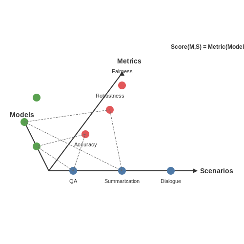
The Holistic Evaluation of Language Models (HELM) framework provides a standardized, multi-dimensional approach to assessing language model performance across diverse tasks, domains, and metrics. Unlike traditional benchmarks that focus narrowly on accuracy or perplexity, HELM systematically evaluates models along three axes: scenarios, metrics, and models.
Core Components of HELM
HELM decomposes evaluation into three primary dimensions:
- Scenarios: A scenario defines a specific task (e.g., question answering, summarization) and dataset (e.g., SQuAD, CNN/DailyMail). HELM includes 42 core scenarios spanning 16 categories, ensuring broad coverage of linguistic capabilities.
- Metrics: Each scenario is evaluated using multiple metrics (e.g., accuracy, robustness, fairness, efficiency). HELM aggregates over 30 distinct metrics, including task-specific measures (e.g., BLEU, ROUGE) and general criteria (e.g., latency, carbon footprint).
- Models: The framework supports evaluation of diverse model families (e.g., GPT-3, PaLM, T5) under controlled conditions, enabling direct comparisons across architectures and scales.
Mathematical Formalization
For a given scenario S and model M, HELM computes a normalized score across N metrics:
where wi are metric-specific weights (defaulting to 1/N for uniform weighting) and norm is a min-max normalization function scaling all metrics to [0,1]. The framework also computes cross-scenario aggregates:
Key Innovations
HELM introduces several methodological advances:
- Standardized Prompts: All evaluations use carefully designed, reproducible prompts to minimize variance from prompt engineering.
- Multiple Input Samples Each test case is evaluated with multiple input formulations to assess robustness to paraphrasing.
- Calibration Metrics Includes expected calibration error (ECE) to measure whether model confidence aligns with actual accuracy.
Implementation Considerations
The HELM benchmark requires:
- Execution on fixed hardware (typically NVIDIA A100 GPUs) for fair latency comparisons
- Multiple random seeds to compute variance estimates
- Strict version control for datasets, models, and evaluation code
Results are typically visualized through radar charts showing performance across metrics, enabling quick identification of model strengths and weaknesses. The framework has revealed critical insights, such as the trade-off between accuracy and robustness in larger models, and has become a standard reference for comprehensive LLM evaluation.
BIG-bench: Beyond the Imitation Game
Overview and Scope
The BIG-bench (Beyond the Imitation Game benchmark) represents a collaborative effort to push the boundaries of language model evaluation through a diverse set of challenging tasks. Unlike traditional benchmarks that focus on narrow capabilities, BIG-bench comprises 204 tasks spanning linguistics, mathematics, commonsense reasoning, and social bias detection. Each task is designed to probe specific aspects of model performance, ranging from simple pattern recognition to complex multi-step reasoning.
Task Design and Categorization
Tasks in BIG-bench are categorized along several dimensions:
- Skill type: Logical reasoning, linguistic understanding, world knowledge, etc.
- Difficulty level: From elementary to expert-human level
- Evaluation metric: Accuracy, BLEU score, F1 score, or custom metrics
For example, the "Dyck Languages" task evaluates a model's ability to process nested structures in formal languages, while "Temporal Sequences" tests understanding of event ordering. The mathematical reasoning tasks often require deriving relationships between variables:
Key Innovations
BIG-bench introduces several methodological advances:
- Human baseline comparison: Each task includes human performance metrics
- Task scaling laws: Studies how performance varies with model size
- Cross-task analysis: Identifies correlations between different capabilities
Implementation Challenges
Evaluating models on BIG-bench presents unique technical challenges:
- Prompt engineering: Many tasks require careful few-shot prompt design
- Computational cost: Full evaluation can require thousands of GPU hours
- Metric alignment: Some tasks require custom evaluation functions
The benchmark's Python API allows for standardized evaluation across models:
from bigbench.api import json_task
task = json_task.JsonTask(task_path="tasks/dyck_languages")
results = task.evaluate_model(model)
Research Insights
Analysis of BIG-bench results has revealed several important findings about LLMs:
- Performance scales predictably with model size for some tasks but not others
- There exist distinct capability clusters that tend to co-develop
- Human-like performance often requires different architectures beyond pure scaling
For instance, the relationship between model size and performance on mathematical tasks follows a power law:
where N is the number of parameters, and α, β, c are task-specific constants.
Current Limitations
While comprehensive, BIG-bench has several limitations researchers should consider:
- Some tasks exhibit ceiling effects for state-of-the-art models
- The benchmark doesn't fully capture real-world deployment scenarios
- Task diversity makes aggregate scoring challenging
3. Selecting Appropriate Benchmarks for Specific Tasks
3.1 Selecting Appropriate Benchmarks for Specific Tasks
Benchmark selection for evaluating large language models (LLMs) requires careful alignment between the benchmark's design and the target task's requirements. Mismatched benchmarks can lead to misleading performance assessments, either overestimating or underestimating a model's capabilities. Key considerations include the benchmark's coverage of relevant skills, its difficulty distribution, and its resistance to dataset contamination or shortcut learning.
Task-Benchmark Alignment Criteria
Effective benchmark selection follows three primary criteria:
- Skill Coverage: The benchmark must comprehensively assess the specific capabilities required for the target task. For question answering, this includes reading comprehension, reasoning, and factual knowledge retrieval.
- Difficulty Distribution: A well-designed benchmark contains items spanning the full spectrum of expected performance levels, from basic to expert, with appropriate weighting.
- Contamination Resistance: The benchmark should minimize the risk of test set leakage during training through careful dataset construction and, when possible, dynamic question generation.
Quantitative Alignment Metrics
The alignment between a benchmark B and target task T can be quantified using mutual information:
where H(B) represents the entropy of benchmark scores and H(B|T) the conditional entropy given task performance. Higher values indicate better alignment. In practice, this is estimated through:
Domain-Specific Benchmark Selection
Different application domains require specialized benchmark suites:
Scientific Reasoning
The SciBench framework evaluates multi-step reasoning through:
- Mathematical derivation problems
- Experimental design analysis
- Literature synthesis tasks
Legal Analysis
Legal application benchmarks focus on:
- Precedent retrieval accuracy
- Statutory interpretation consistency
- Argument structure evaluation
Dynamic Benchmark Adaptation
For evolving tasks, static benchmarks become outdated quickly. Adaptive benchmarks address this through:
where the benchmark updates based on model performance gradients ∇θL on new data Dnew. This approach maintains relevance as both models and task requirements evolve.
Benchmark Quality Assessment
The quality of a benchmark can be evaluated through its:
- Discriminative Power: Ability to distinguish between models of different capability levels
- Robustness: Resistance to gaming through prompt engineering or other non-generalizable techniques
- Representativeness: Coverage of the task's real-world complexity distribution
These properties can be quantified through statistical measures like the benchmark's Gini coefficient for discriminative power and its Jensen-Shannon divergence from real task distributions.
3.2 Ensuring Fair Comparison Across Models
Comparing large language models (LLMs) requires strict standardization to avoid confounding variables that distort performance metrics. Key factors include computational constraints, training data contamination, prompt engineering, and evaluation protocols. Without controlling these variables, benchmark results become unreliable for assessing true model capabilities.
Computational Resource Normalization
Model performance scales nonlinearly with compute budget, making direct comparisons unfair unless normalized. The scaling law for autoregressive transformers is given by:
Where N is parameters, D is training tokens, and L∞ represents irreducible loss. To compare models trained with different budgets, we solve for equivalent scaling:
This allows projecting performance to a standardized compute baseline (e.g., 1e24 FLOPs). Recent work suggests αN ≈ 0.076 and αD ≈ 0.095 for dense transformers.
Data Contamination Controls
Benchmark leakage into training data artificially inflates scores. Detection methods include:
- N-gram overlap analysis with Jaccard similarity thresholding
- Embedding-based retrieval using FAISS index of benchmark questions
- Perplexity delta testing comparing benchmark vs. holdout text
The contamination probability Pc can be modeled as:
Where fi is n-gram frequency and T is corpus size. Models exceeding Pc > 0.05 should be flagged.
Prompt Engineering Parity
LLM performance varies dramatically with prompt formatting. Standardized comparison requires:
- Identical few-shot exemplars across models
- Fixed template structures (e.g., "Question: {q}\nAnswer:")
- Controlled output constraints (max tokens, sampling temperature)
The prompt sensitivity metric Sp quantifies variance across formulations:
Where Ai is accuracy across n prompt variants. High Sp indicates unreliable benchmarking.
Evaluation Protocol Consistency
Key standardization requirements include:
- Identical answer post-processing (whitespace normalization, casing rules)
- Fixed random seeds for stochastic evaluations
- Standardized hardware (avoiding quantization artifacts)
- Multiple inference passes for confidence intervals
Statistical significance testing should use paired bootstrap resampling with:
Where z is the critical value for 95% confidence. Differences are only meaningful if |δ| > 2σ.
3.3 Addressing Data Contamination Issues
Data contamination occurs when a language model's training data overlaps with its evaluation benchmarks, leading to artificially inflated performance metrics. This issue is particularly problematic in large-scale LLM evaluations, where models trained on vast internet corpora may inadvertently memorize or reproduce benchmark-specific patterns. Detecting and mitigating contamination requires rigorous methodological controls.
Detecting Contamination Through N-Gram Analysis
One approach involves analyzing the overlap between training data and benchmark questions at the n-gram level. For a given benchmark dataset B and training corpus T, the contamination risk C for n-grams of length k can be quantified as:
where Bk and Tk represent the sets of all k-length n-grams in the benchmark and training data, respectively. Values approaching 1 indicate high contamination risk. In practice, researchers often examine multiple n-gram lengths (typically 3 ≤ k ≤ 10) to capture different levels of memorization.
Dynamic Benchmarking Strategies
To circumvent contamination, dynamic benchmarking methods have emerged:
- Adversarial Example Generation: Modifying benchmark questions while preserving their semantic content using paraphrasing or synonym substitution.
- Temporal Separation: Using benchmarks published after the model's training data cutoff date.
- Controlled Subsampling: Creating evaluation subsets with minimal n-gram overlap with known training sources.
Statistical Significance Testing
When contamination is suspected, permutation tests can assess whether observed performance improvements are statistically significant. For a model with accuracy a on benchmark B, we compute:
where ai are accuracies on N randomly permuted versions of B, and I is the indicator function. Small p-values (typically < 0.05) suggest the model's performance may stem from contamination rather than genuine understanding.
Practical Implementation Considerations
In real-world evaluations, several best practices have emerged:
- Maintaining strict separation between training and evaluation data pipelines
- Implementing automated checks for n-gram overlap during dataset construction
- Reporting detailed data provenance for all benchmarks
- Using multiple diverse benchmarks to cross-validate results
Recent studies suggest that even minimal contamination (overlap < 1%) can inflate performance metrics by 5-15% on certain benchmarks, emphasizing the need for rigorous controls in high-stakes evaluations.
4. Evaluating Few-shot and Zero-shot Learning
Evaluating Few-shot and Zero-shot Learning
Performance Metrics for Few-shot Learning
Few-shot learning evaluates a model's ability to generalize from a minimal set of labeled examples, typically k samples per class (k-shot learning). The primary metric is few-shot accuracy, computed as:
where N is the total number of test samples, ŷi is the predicted label, and yi is the ground truth. For regression tasks, mean squared error (MSE) is used:
Zero-shot Evaluation Protocols
Zero-shot learning measures a model's ability to infer unseen classes without training examples, relying solely on auxiliary information (e.g., class attributes or textual descriptions). Key metrics include:
- Harmonic Mean (H): Balances seen (S) and unseen (U) class accuracy to avoid bias:
$$ H = \frac{2 \times \text{Acc}_S \times \text{Acc}_U}{\text{Acc}_S + \text{Acc}_U} $$
- Generalized Zero-shot Accuracy: Evaluates performance on both seen and unseen classes simultaneously.
Benchmark Datasets
Standardized datasets enable reproducible comparisons:
- Few-shot: Mini-ImageNet (64/16/20 split for train/val/test classes), Omniglot (1,623 characters with 20 samples each).
- Zero-shot: AWA2 (50 animal classes with 85 attributes), CUB (200 bird species with 312 attributes).
Challenges and Pitfalls
Evaluation must account for:
- Data leakage: Pre-training on datasets overlapping with benchmark test classes.
- Prompt sensitivity: Zero-shot performance varies significantly with input phrasing.
- Calibration: Models may exhibit overconfidence in few/zero-shot predictions, requiring temperature scaling.
Case Study: GPT-3's Few-shot Performance
On the LAMBADA dataset (word prediction task), GPT-3 achieves 76% accuracy in a 32-shot setting versus 45% in zero-shot, demonstrating the impact of in-context examples. The performance follows a log-linear trend with shot count:
where α and β are dataset-specific coefficients.
4.2 Assessing Bias and Fairness in LLMs
Quantifying Bias in Language Models
Bias in LLMs manifests as skewed probability distributions over tokens or sequences correlated with protected attributes like gender, race, or religion. To measure this, we define disparate impact as the ratio of conditional probabilities for sensitive versus non-sensitive groups:
where w is a target word or phrase, and a is a binary protected attribute. A DI value deviating significantly from 1 indicates bias. For continuous attributes (e.g., sentiment polarity), we use demographic parity difference:
Benchmark Datasets and Metrics
Common benchmarks include:
- StereoSet: Measures stereotypical associations via context-aware scoring
- BiasNLI: Evaluates entailment judgments across demographic pairs
- HolisticBias: Tests 600+ identity dimensions through template-based probes
The Bias Score for a model M on dataset D is computed as:
Causal Analysis of Bias Propagation
Bias emerges from three primary sources in the training pipeline:
- Data bias: Skewed co-occurrence statistics in pretraining corpora
- Architectural bias: Attention mechanisms amplifying certain patterns
- Objective bias: Loss functions optimizing for majority-group performance
We can isolate these components using counterfactual probing. For a given input x, generate counterfactuals x' by perturbing protected attributes while holding other features constant. The bias attribution is:
Mitigation Techniques
Advanced debiasing approaches include:
- Adversarial forgetting: Gradient reversal during fine-tuning
- Concept erasure: Null-space projection of sensitive directions
- Counterfactual data augmentation: Generating balanced synthetic examples
The effectiveness of mitigation is evaluated using minimum description length of the fairness-accuracy tradeoff:
where θbias represents the subset of parameters most influential on bias-related outputs.
4.3 Measuring Robustness and Adversarial Performance
Adversarial Attack Formulation
Adversarial attacks on language models involve perturbing inputs to induce incorrect outputs while preserving semantic meaning. Let x be the original input and x' the adversarial variant. The attack objective is:
where f is the model, y the true label, ℒ the loss function, and sim a semantic similarity metric with threshold ε. Common perturbation strategies include:
- Character-level: Typos, homoglyphs, Unicode substitutions
- Token-level: Synonym replacements, paraphrasing
- Structural: Word order changes, syntactic transformations
Robustness Metrics
Three key metrics quantify model robustness under adversarial conditions:
1. Adversarial Success Rate (ASR)
Where N is the number of test cases and 𝕀 the indicator function. ASR measures attack effectiveness.
2. Semantic Preservation Score (SPS)
Computes the similarity between original and adversarial outputs using metrics like:
- BERTScore: Contextual embedding cosine similarity
- BLEURT: Learned evaluation metric for text generation
- ROUGE-L: Longest common subsequence alignment
3. Robust Accuracy Drop (RAD)
Quantifies performance degradation under attack conditions compared to clean inputs.
Benchmarking Methodologies
Standardized evaluation frameworks include:
ANLI (Adversarial Natural Language Inference)
Tests logical reasoning robustness through adversarial premise-hypothesis pairs. Measures consistency in label prediction under carefully crafted contradicting examples.
AdvGLUE
Extends GLUE benchmark with adversarial variants across multiple NLP tasks. Evaluates both task performance and transferability of attacks across domains.
CheckList
Behavioral testing framework assessing capabilities like:
- Vocabulary invariance (synonym robustness)
- Negation robustness
- Logical consistency
Defensive Evaluation Protocols
When assessing defense mechanisms, follow these experimental best practices:
- Adaptive Attacks: Evaluate against white-box attacks with full defense knowledge
- Transfer Attacks: Test generalization to unseen attack methods
- Clean Performance Preservation: Verify defenses don't degrade normal operation
- Compute Efficiency: Measure inference latency overhead
Recent work suggests using certified robustness bounds for provable guarantees. For a text classifier with Lipschitz constant L, the certified radius r guarantees correct classification within:
where δ is the minimum margin between top class predictions.
5. Setting Up Evaluation Pipelines
5.1 Setting Up Evaluation Pipelines
Evaluation pipelines for large language models (LLMs) require systematic design to ensure reproducibility, scalability, and interpretability. A robust pipeline consists of four core components: data preprocessing, model inference, metric computation, and results aggregation. Each component must be modular to accommodate diverse benchmarks like GLUE, SuperGLUE, or HELM.
Data Preprocessing
Raw benchmark datasets often require normalization to ensure compatibility with the target LLM. For text-based tasks, this includes tokenization (using the model’s native tokenizer), truncation/padding to uniform sequence lengths, and encoding categorical labels. For example, Hugging Face’s datasets library standardizes this process:
from transformers import AutoTokenizer
tokenizer = AutoTokenizer.from_pretrained("meta-llama/Llama-2-7b")
def preprocess(examples):
    return tokenizer(examples["text"], truncation=True, padding="max_length", max_length=512)
Model Inference
Inference must be optimized for throughput and memory efficiency. Techniques like dynamic batching (grouping inputs by length) and mixed-precision inference (FP16/INT8) reduce latency. For distributed evaluation across GPUs, frameworks like PyTorch’s DistributedDataParallel synchronize predictions:
where \( t_i \) is the latency for batch \( i \), and \( B \) is the total number of batches.
Metric Computation
Task-specific metrics (e.g., BLEU, ROUGE, accuracy) should be decoupled from model logic to allow flexible benchmarking. Libraries like evaluate provide standardized implementations:
import evaluate
bleu = evaluate.load("bleu")
results = bleu.compute(predictions=preds, references=refs)
Results Aggregation
Statistical significance testing (e.g., bootstrapping or paired t-tests) is critical for comparing models. For a dataset with \( N \) samples, bootstrap resampling involves:
where \( \hat{\theta} \) is the metric estimate and \( \text{SE} \) is the standard error across resampled splits.
Pipeline Orchestration
Tools like Apache Beam or Metaflow enable scalable pipeline execution across cloud clusters. A well-designed pipeline logs artifacts (predictions, metrics) and supports incremental evaluation to avoid reprocessing unchanged data.

5.2 Interpreting Benchmark Results
Statistical Significance and Confidence Intervals
When comparing LLM benchmark scores, statistical significance must be evaluated to determine whether observed differences reflect true model capabilities or random variation. For a dataset with N samples, the standard error of the mean (SEM) is calculated as:
where σ is the standard deviation of the metric scores. The 95% confidence interval for the mean score μ then becomes:
Overlapping confidence intervals between models suggest that performance differences may not be statistically significant. For example, if Model A scores 85.3 ± 1.2 and Model B scores 86.1 ± 1.4, the difference is not statistically significant at p < 0.05.
Normalization and Cross-Dataset Comparability
Benchmark scores often require normalization when comparing across datasets with different scales. Z-score normalization is commonly applied:
where x is the raw score, and μbaseline and σbaseline are the mean and standard deviation of a reference model's scores. This enables meaningful comparison between benchmarks like GLUE (0-100 scale) and SuperGLUE (0-1 scale).
Task-Specific Metric Interpretation
Different NLP tasks require specialized interpretation approaches:
- Text generation: Perplexity (PPL) should be analyzed alongside human evaluation scores, as low PPL doesn't guarantee high-quality output.
- Question answering: Exact match (EM) and F1 scores must be weighted by answer length and ambiguity.
- Reasoning tasks: Accuracy alone is insufficient; error analysis should categorize mistakes into logical, factual, or comprehension errors.
Bias and Artifact Detection
Benchmark results may be inflated by dataset artifacts or unintended biases. The following techniques help detect such issues:
A high artifact score (> 0.3) suggests the model is exploiting dataset biases rather than demonstrating true capability. For example, on the SNLI dataset, some models achieve high accuracy by matching hypothesis words to premise words without understanding logical relationships.
Scaling Laws and Compute-Normalized Performance
When comparing models with different computational budgets, performance should be evaluated relative to the scaling law expectation:
where N is the number of parameters, L0 is the irreducible loss, and α is the scaling exponent (typically ~0.07 for LLMs). A model that significantly outperforms this curve may represent a genuine architectural improvement rather than simply benefiting from increased scale.
Cross-Modal Benchmark Alignment
For multimodal models, benchmark scores must be interpreted in the context of alignment between modalities. The modality alignment score can be computed as:
where K is the number of task pairs. A MAS approaching 1 indicates strong cross-modal understanding, while lower scores suggest modality-specific optimization without true integration.
5.3 Common Pitfalls and How to Avoid Them
Overfitting to Benchmark Metrics
Many LLMs exhibit benchmark overfitting, where models are optimized specifically for test-set performance without genuine generalization. This often occurs when training data inadvertently leaks into validation sets or when models exploit superficial patterns in benchmark construction. For example, models fine-tuned on GLUE or SuperGLUE may achieve high scores by memorizing syntactic cues rather than learning semantic understanding.
To mitigate this:
- Use out-of-distribution evaluation on unseen datasets with similar tasks
- Implement adversarial perturbations to test robustness against minor input variations
- Apply cross-dataset validation where training and test data come from different sources
Ignoring Computational Efficiency
Benchmarks often prioritize accuracy while neglecting computational costs. A model achieving state-of-the-art results may require impractical resources (e.g., 1,024 GPUs for inference). The Pareto frontier between performance and efficiency can be quantified as:
Practical solutions include:
- Reporting latency-throughput curves alongside accuracy metrics
- Using hardware-aware benchmarks like MLPerf Inference
- Incorporating energy consumption metrics (watts per prediction)
Data Contamination
Pre-training datasets often contain benchmark test samples, leading to inflated performance. For instance, The Pile dataset was found to include 3.2% of HumanEval Python problems. Detection methods involve:
Where Ti represents benchmark test sets. Prevention strategies:
- Implement data de-duplication using cryptographic hashing of test samples
- Perform canary sequences analysis to detect memorization
- Use differential evaluation comparing performance on known-clean vs. suspected-contaminated data
Metric Gaming
Models can exploit metric weaknesses without true capability improvement. For example:
- BLEU rewards lexical overlap over semantic correctness
- ROUGE favors longer outputs regardless of relevance
- Accuracy metrics fail on imbalanced datasets
Countermeasures include:
- Employing ensemble metrics (e.g., BLEURT, MoverScore)
- Adding human evaluation for subjective tasks
- Using worst-case subgroup analysis to identify failure modes
Temporal Drift
Static benchmarks become obsolete as models improve. The benchmark decay rate can be modeled as:
Where S(t) is benchmark usefulness and ε(t) represents new capabilities. Solutions:
- Implement dynamic benchmarks with automated difficulty scaling
- Use adversarial data collection to continuously expand test cases
- Adopt meta-evaluation protocols to assess benchmark quality itself
Cultural and Linguistic Bias
Most benchmarks focus on English and Western contexts. For multilingual evaluation:
- Test cross-lingual transfer performance using XTREME or XNLI
- Measure dialectal variance through datasets like Arabic Dialect Identification
- Evaluate cultural alignment using localized versions of ethical benchmarks
6. Key Research Papers on LLM Evaluation
6.1 Key Research Papers on LLM Evaluation
- LLMs-as-Judges: A Comprehensive Survey on LLM-based Evaluation Methods — Despite its great potential and significant advantages, LLMs-as-judges also face several critical challenges. For example, the evaluation results of LLMs are often influenced by the prompt template, which can lead to biased or inconsistent assessments (Xu et al., 2023a).Considering that LLMs are trained on extensive text corpus, they may also inherit various implicit biases, impacting the ...
- PDF Benchmarking LLMs on Advanced Mathematical Reasoning — Figure 4.1: Sample (Question, Answer, Rubric) tuple for evaluating LLM-as-a-judge. Cor-respondence between the solution and LLM-generated rubric is shown in color 4.1 Evaluation We evaluate each of the aforementioned LLM-as-a-judge frameworks using the dataset of 100 student answers from the undergraduate linear algebra course. The primary metric
- A Systematic Survey and Critical Review on Evaluating — To initiate the evaluation process of LLMs, the first step is selecting appropriate benchmarks. We categorize the benchmarking datasets into the following: general capability benchmarks, specialized benchmarks, and other diverse benchmarks.We refer to general capability benchmarks as the ones that are often used for evaluation upon the release of an LLM (e.g., MMLU Hendrycks et al ...
- A Survey on Evaluation of Large Language Models — This paper presents the first survey to give a comprehensive overview of the evaluation on LLMs from three aspects: what to evaluate, how to evaluate, and where to evaluate. By encapsulating evaluation tasks, protocols, and benchmarks, our aim is to augment understanding of the current status of LLMs, elucidate their strengths and limitations ...
- tinyBenchmarks: evaluating LLMs with fewer examples - arXiv.org — Large Language Models (LLMs) have demonstrated remarkable abilities to solve a diverse range of tasks (Brown et al., 2020).Quantifying these abilities and comparing different LLMs became a challenge that led to the development of several key benchmarks, e.g., MMLU (Hendrycks et al., 2020), Open LLM Leaderboard (Beeching et al., 2023), HELM (Liang et al., 2022), and AlpacaEval (Li et al., 2023).
- Large language models (LLMs): survey, technical frameworks ... - Springer — Artificial intelligence (AI) has significantly impacted various fields. Large language models (LLMs) like GPT-4, BARD, PaLM, Megatron-Turing NLG, Jurassic-1 Jumbo etc., have contributed to our understanding and application of AI in these domains, along with natural language processing (NLP) techniques. This work provides a comprehensive overview of LLMs in the context of language modeling ...
- Are LLMs good at structured outputs? A benchmark for evaluating ... — For the research community, This study makes significant contributions to the research field of evaluating LLMs' structured output capabilities. By developing the SoEval benchmark, we establish a standardized framework for assessing and comparing the performance of various models in generating structured outputs, laying the foundation for ...
- Evaluating Large Language Models: A Comprehensive Survey - ar5iv — To enable more comprehensive LLM assessment, this survey provides a systematic literature review synthesizing efforts to evaluate these models across various dimensions. We summarize key points regarding general LLM benchmarks and evaluation methodologies spanning knowledge, reasoning, tool learning, toxicity, truthfulness, robustness, and privacy.
- Enterprise Benchmarks for Large Language Model Evaluation — The advancement of large language models (LLMs) has led to a greater challenge of having a rigorous and systematic evaluation of complex tasks performed, especially in enterprise applications.
- Large language models encode clinical knowledge - Nature — Large language models (LLMs) have demonstrated impressive capabilities, but the bar for clinical applications is high. Attempts to assess the clinical knowledge of models typically rely on ...
6.2 Open-source Benchmarking Tools
- LLM Benchmarks: Guide to Evaluating Language Models — Developed by Li et al. in April 2023, API-Bank sets the stage for future benchmarks, emphasizing the potential of LLMs when paired with external tools. Dive into the intricacies of this pioneering benchmark in Brad Nikkel's article. The ARC Benchmark: Evaluating LLMs' Reasoning Abilities
- Understanding LLM Evaluation and Benchmarks: A Complete Guide - Turing — H2O LLM EvalGPT: Developed by H2O.ai, this open tool evaluates and compares LLMs, offering a platform to assess model performance across various tasks and benchmarks. It features a detailed leaderboard of high-performance, open-source LLMs, helping you choose the best model for tasks like summarizing bank reports or responding to queries.
- 20 LLM evaluation benchmarks and how they work — FinBen is an open-source benchmark designed to evaluate LLMs in the financial domain. It includes 36 datasets that cover 24 tasks in seven financial domains: information extraction, text analysis, question answering, text generation, risk management, forecasting, and decision-making. ... LLM benchmarks are a powerful tool for evaluating the ...
- Title: tinyBenchmarks: evaluating LLMs with fewer examples - arXiv.org — The versatility of large language models (LLMs) led to the creation of diverse benchmarks that thoroughly test a variety of language models' abilities. These benchmarks consist of tens of thousands of examples making evaluation of LLMs very expensive. In this paper, we investigate strategies to reduce the number of evaluations needed to assess the performance of an LLM on several key ...
- tinyBenchmarks: evaluating LLMs with fewer examples - arXiv.org — For example, we show that to accurately estimate the performance of an LLM on MMLU, a popular multiple-choice QA benchmark consisting of 14K examples, it is sufficient to evaluate this LLM on 100 curated examples. We release evaluation tools and tiny versions of popular benchmarks: Open LLM Leaderboard, MMLU, HELM, and AlpacaEval 2.0.
- Large Language Model Evaluation in 2025: 5 Methods - AIMultiple — They usually offer defined benchmarks, test suites, and reporting systems to evaluate LLMs across a range of capabilities and dimensions. LEval (Language Model Evaluation) is a framework for evaluating LLMs on long-context understanding. 13 LEval is a benchmark suite featuring 411 questions across eight tasks, with contexts from 5,000 to ...
- \benchmarkname : A Benchmark for LLMs as Intelligent Agents - arXiv.org — Taking a unique agent perspective in benchmarking LLMs, we introduce \benchmarkname, a benchmark from 6 distinct games augmented with language descriptors for visual observation (Figure 1), offering up to 20 different settings and infinite environment variations.Each game presents unique challenges that span multiple dimensions of intelligent agents, as detailed in Table 3.
- GitHub - openai/evals: Evals is a framework for evaluating LLMs and LLM ... — You can find the full instructions to run existing evals in run-evals.md and our existing eval templates in eval-templates.md.For more advanced use cases like prompt chains or tool-using agents, you can use our Completion Function Protocol.. We provide the option for you to log your eval results to a Snowflake database, if you have one or wish to set one up.
- Evaluating LLM systems: Metrics, challenges, and best practices — The golden dataset serves as a benchmark, providing a reliable standard for evaluating the LLM's capabilities, identifying areas of improvement, and aligning it with the intended use case.
6.3 Recommended Books and Surveys
- Evaluating Large Language Models: A Comprehensive Survey — API-Bank (Li et al., 2023c) presents a tailor-made benchmark for evaluating tool-augmented LLMs, encompassing 53 standard API tools, a comprehensive workflow for tool-augmented LLMs, and 264 annotated dialogues. It uses accuracy as a metric for evaluating API calls, ROUGE-L as a metric for evaluating post-call responses.
- A Systematic Survey and Critical Review on Evaluating — To initiate the evaluation process of LLMs, the first step is selecting appropriate benchmarks. We categorize the benchmarking datasets into the following: general capability benchmarks, specialized benchmarks, and other diverse benchmarks.We refer to general capability benchmarks as the ones that are often used for evaluation upon the release of an LLM (e.g., MMLU Hendrycks et al ...
- (PDF) Trustworthy LLMs: a Survey and Guideline for Evaluating Large ... — Trustworthy LLMs: a Survey and Guideline for Evaluating Large Language Models' Alignment. ... 6. 3 P r e f e r e n c e B i a s ... Our goal is not to benchmark or rank all available methods, but ...
- Are LLMs good at structured outputs? A benchmark for evaluating ... — Existing evaluation benchmarks assess LLMs in general or specialized domains, but they often overlook the models' ability to produce structured outputs. ... "Book", "author": "Author"} Triples: ... A survey on evaluation of large language models (2023) arXiv preprint arXiv:2307.03109. Google Scholar. Chen et al., 2021.
- LLMs in Production[Book] - O'Reilly Media — You'll learn techniques for preparing an LLM dataset, cost-efficient training hacks like LORA and RLHF, and industry benchmarks for model evaluation. Along the way, you'll put your new skills to use in three exciting example projects: creating and training a custom LLM, building a VSCode AI coding extension, and deploying a small model to a ...
- (PDF) AgentBench: Evaluating LLMs as Agents - ResearchGate — LLMs and their competitive scores on sev eral benchmarks [], their performance on the challenging 2 T able 1: AgentBench evaluates 25 API-based or open-sourced LLMs on LLM-as-Agent challenges.
- PDF Are LLMs good at structured outputs? A benchmark for evaluating ... — Note: The survey involved a total of 100 participants, selected through purposive sampling to ensure representation from various industries. The participants were chosen based on their professional roles. Existing evaluation benchmarks assess LLMs in general or specialized domains, but they often overlook the models' ability to
- PM-LLM-Benchmark: Evaluating Large Language Models on ... - Springer — The benchmark focuses on two implementation paradigms, i.e., the direct provision of insights and code generation.Moreover, specific focus is given on process-mining-specific and process-specific domain knowledge, which is required for the considered prompts.Other available lists of process mining inquiries, such as the ones proposed in [], are based on the generation of SQL statements but do ...
- PDF LexEval: A Scalable LLM Evaluation Framework - Imperial College London — the continuous advancements in language models. It enables users to fine-tune their evaluation paradigms, focusing on lexical or paraphrasing perturbations as required. Our extensive testing of 7 LLMs includes comprehensive performance documentation, detailed RAG pipeline failure analysis, and qualitative response assessments.
- Building LLM Applications: Evaluation (Part 8) - Medium — Learn Large Language Models ( LLM ) through the lens of a Retrieval Augmented Generation ( RAG ) Application. · 1. Overview · 2. LLM Benchmarking Vs. Evaluation · 3. LLM Benchmarking · 3.1.