Knowledge Distillation for LLMs
1. Definition and Core Principles
Definition and Core Principles
Knowledge distillation is a model compression technique where a smaller, more efficient student model is trained to replicate the behavior of a larger, more complex teacher model. Originally introduced by Buciluǎ et al. (2006) and later formalized by Hinton et al. (2015), the method leverages the teacher's soft probability outputs—rather than hard labels—to transfer nuanced knowledge, including learned relationships between classes and generalization patterns.
Mathematical Formulation
The core objective of knowledge distillation is to minimize the divergence between the teacher's and student's output distributions. Given a teacher model T and a student model S, the distillation loss Ldistill is typically formulated using Kullback-Leibler (KL) divergence:
where T(xi) and S(xi) are the softened logits (using temperature scaling) of the teacher and student, respectively, for input xi. The temperature parameter τ controls the smoothness of the output distribution:
Key Components
- Soft Targets: The teacher's probabilistic outputs preserve inter-class relationships (e.g., "cat" and "dog" may have higher co-probability than "cat" and "airplane").
- Temperature Scaling: Higher τ values produce smoother distributions, emphasizing relative probabilities over absolute confidence.
- Loss Composition: Often combined with traditional cross-entropy loss (LCE) for balanced learning: L = αLCE + (1-α)Ldistill, where α is a weighting hyperparameter.
Practical Considerations
For large language models (LLMs), knowledge distillation must address scalability challenges. Techniques like layer-wise distillation (transferring intermediate representations) and task-specific distillation (focusing on downstream performance) are common. Recent advances also explore dynamic distillation, where the teacher's role adapts during training.
Empirical studies show that distilled LLMs can retain >90% of the teacher's performance while reducing parameter counts by 10-100x. For example, DistilBERT (Sanh et al., 2019) achieves 97% of BERT's accuracy with 40% fewer parameters, demonstrating the method's efficacy.
1.2 Teacher-Student Model Paradigm
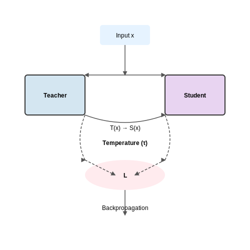
The teacher-student model paradigm in knowledge distillation is a framework where a large, pre-trained model (the teacher) transfers its learned knowledge to a smaller, more efficient model (the student). This process is particularly valuable for deploying large language models (LLMs) in resource-constrained environments while preserving performance.
Mechanism of Knowledge Transfer
The teacher model generates soft targets—probability distributions over output classes—rather than hard labels. These soft targets capture the teacher's nuanced understanding of the data, including relationships between classes that are not evident in one-hot encoded labels. The student model is trained to mimic these soft targets, often using a loss function that combines:
- Distillation loss: Measures the divergence between teacher and student soft targets.
- Student loss: Ensures the student performs well on the original labeled data.
The combined loss function is typically formulated as:
where α balances the contributions of the two losses.
Temperature Scaling
To soften the probability distributions further, a temperature parameter T is applied to the logits before the softmax operation:
Higher values of T produce smoother distributions, emphasizing the relative differences between classes. During training, T is typically set greater than 1, while at inference, it reverts to 1 for sharp predictions.
Architectural Considerations
The teacher and student models can differ significantly in architecture, but the student must be capable of approximating the teacher's behavior. Common strategies include:
- Layer-wise distillation: Aligning intermediate representations between teacher and student layers.
- Attention transfer: Matching attention maps in transformer-based models to preserve contextual focus.
- Dynamic teacher ensembles: Leveraging multiple teachers to provide diverse supervisory signals.
Practical Applications
This paradigm has been successfully applied to compress LLMs like BERT into smaller variants (e.g., DistilBERT, TinyBERT), achieving comparable performance with significantly reduced computational costs. Recent advancements explore cross-modal distillation, where teachers and students operate on different data modalities (e.g., text-to-speech models).
Mathematical Derivation of Gradient Flow
The gradient of the distillation loss with respect to the student's logits z_i can be derived as:
where q_i and p_i are the softened probabilities of the teacher and student, respectively. This gradient encourages the student to adjust its predictions toward the teacher's distribution.

1.3 Key Components: Logits, Soft Targets, and Temperature Scaling
Logits: The Foundation of Knowledge Distillation
Logits are the raw, unnormalized output values produced by the final layer of a neural network before applying any activation function. In the context of large language models (LLMs), logits represent the model's confidence scores for each possible token in the vocabulary. Given an input sequence x, the logits z are computed as:
where W is the weight matrix, h is the hidden state, and b is the bias term. These logits are critical in knowledge distillation because they contain the full information about the teacher model's predictions, including relative confidence across classes.
Soft Targets: Probabilistic Knowledge Transfer
Soft targets are generated by applying the softmax function to the logits, converting them into a probability distribution over the output classes (or tokens in LLMs). The standard softmax function is defined as:
where N is the number of classes (or vocabulary size). In knowledge distillation, soft targets serve as a richer training signal than hard labels (one-hot vectors) because they capture the teacher model's learned relationships between classes. For example, in machine translation, the teacher's soft targets might indicate that "cat" and "feline" are similarly plausible translations, whereas a hard label would only specify one correct answer.
Temperature Scaling: Controlling Distribution Smoothness
Temperature scaling modifies the softmax function to control the sharpness of the output distribution. The temperature-scaled softmax is given by:
where T is the temperature hyperparameter. The effect of temperature scaling can be understood through three regimes:
- T = 1: Standard softmax, preserving the original distribution shape
- T > 1: Smoother distribution, emphasizing relative differences between non-maximal classes
- T < 1: Sharper distribution, approaching a one-hot encoding as T → 0
In practice, temperature values between 2 and 10 are commonly used during distillation. Higher temperatures are particularly valuable when:
- The teacher model's predictions are overly confident (low entropy)
- The task benefits from emphasizing secondary patterns (e.g., capturing synonyms in language tasks)
- Distilling from very large teachers to much smaller students
Practical Implementation Considerations
The distillation loss typically combines two terms:
where α balances between the soft target loss (usually KL divergence) and the standard cross-entropy loss with ground truth labels. The temperature is applied only to the soft targets during training, while inference uses T=1.
Modern implementations often employ adaptive temperature scheduling, where T is gradually decreased during training. This approach mirrors curriculum learning, starting with easier-to-learn smoothed distributions before focusing on finer distinctions.
Advanced Variants and Recent Developments
Recent work has explored several enhancements to the basic temperature scaling approach:
- Layer-wise Temperature: Applying different temperatures to different layers of the teacher network
- Dynamic Temperature: Automatically adjusting T based on batch statistics or learning progress
- Multi-temperature Distillation: Using multiple temperature settings simultaneously and combining their outputs
These methods have shown particular promise in distilling very large language models (e.g., GPT-3 or PaLM) where the original logit distributions are extremely sharp (entropy < 1 nats in many cases).

2. Challenges in Distilling LLMs
Challenges in Distilling LLMs
Model Size and Computational Overhead
Large Language Models (LLMs) often contain billions of parameters, making direct distillation computationally prohibitive. The teacher model's forward pass alone may require multiple GPUs, while the student model must replicate this behavior with significantly fewer resources. The computational complexity scales with the sequence length n as O(n²) due to self-attention mechanisms, exacerbating memory constraints during training.
where d represents the hidden dimension. For a 175B parameter model like GPT-3, even a single batch iteration demands terabytes of memory, necessitating specialized parallelism techniques.
Loss Landscape Mismatch
The teacher's output distribution often contains sharp peaks (high-confidence predictions) that the student struggles to approximate. When using Kullback-Leibler (KL) divergence as the distillation loss:
the gradient updates become unstable when piT → 1, causing vanishing gradients for low-probability tokens. Temperature scaling helps mitigate this but introduces hyperparameter sensitivity.
Capacity Gap
Student models with 100x fewer parameters cannot perfectly mimic teacher behavior, leading to:
- Representational collapse: Over-simplification of attention patterns
- Catastrophic forgetting: Loss of generalizability during task-specific distillation
- Mode averaging: Student produces "blurry" versions of teacher outputs
Multi-Modality of Output Distributions
LLMs generate multimodal distributions across:
- Token-level predictions
- Attention heads
- Hidden state dynamics
Standard distillation approaches that only match final layer logits fail to capture intermediate representations critical for few-shot learning. Layer-wise distillation losses must account for:
Dynamic Teacher Behavior
LLMs exhibit context-dependent reasoning patterns that change with:
- Prompt engineering
- Few-shot examples
- Chain-of-thought scaffolding
Static distillation cannot preserve these adaptive capabilities. Recent solutions employ:
- Prompt-conditional distillation
- Mixture-of-experts student architectures
- Reinforcement learning from teacher trajectories
Evaluation Discrepancies
Standard benchmarks (GLUE, SuperGLUE) fail to detect:
- Degradation in compositional generalization
- Loss of calibration under distribution shift
- Reduced robustness to adversarial prompts
Specialized metrics like:
are required to assess distillation quality beyond perplexity.
Architectural Considerations for Student Models
The architecture of the student model in knowledge distillation plays a critical role in determining the efficiency-accuracy trade-off. Unlike traditional model design, student models must balance three competing objectives: parameter efficiency, inference speed, and knowledge retention from the teacher. The optimal architecture depends on the distillation method employed, the teacher model's complexity, and the target deployment constraints.
Depth vs. Width Trade-offs
Empirical studies show that student models benefit more from increased width than depth when distilling knowledge from large transformers. For a teacher model with L layers and hidden dimension d, the student's hidden dimension d' should satisfy:
where C is a compression factor (typically 0.1-0.5). This relationship emerges from the rank preservation requirements for attention head matrices. Shallower but wider architectures better maintain the teacher's representational capacity while reducing computational complexity quadratically with layer count.
Attention Mechanism Variants
For transformer-based students, modified attention mechanisms can achieve significant efficiency gains:
- Factorized Attention: Decomposes the full attention matrix into low-rank products, reducing memory from O(n²) to O(nk) where k ≪ n.
- Local Window Attention: Restricts attention spans to fixed neighborhoods, particularly effective for long-sequence tasks.
- Cross-head Parameter Sharing: Shares key/value projections across attention heads while maintaining unique query transformations.
Feed-Forward Network Design
The student's FFN layers often require careful dimension scaling to preserve the teacher's knowledge. A proven strategy uses bottleneck architectures with expansion ratio r:
with r typically 2-4x smaller than the teacher's expansion ratio. This maintains representational capacity while reducing parameters by O(r²).
Residual Connection Modifications
Student models benefit from learnable residual weights rather than fixed additions:
where αl are trainable scalars. This adaptation helps balance the contribution of each distilled layer, particularly when the student has significantly fewer layers than the teacher.
Embedding Layer Compression
Vocabulary embeddings often constitute 20-40% of LLM parameters. Effective compression techniques include:
- Factorized Embeddings: Decomposes the embedding matrix E ∈ ℝ^{|V|×d} into E = E_1E_2 where E_1 ∈ ℝ^{|V|×k}, E_2 ∈ ℝ^{k×d} (k ≪ d)
- Hash-based Embeddings: Uses multiple hash functions to share parameters across tokens
- Differentiable Product Quantization: Learns a codebook of sub-embeddings combined through soft assignments
These methods typically achieve 4-10x compression with < 2% accuracy drop on downstream tasks when combined with proper distillation.
2.3 Handling Massive Parameter Spaces
Parameter Space Compression via Low-Rank Factorization
The sheer size of modern LLMs, often exceeding hundreds of billions of parameters, makes direct distillation computationally intractable. Low-rank factorization decomposes weight matrices W ∈ ℝm×n into the product of two smaller matrices U ∈ ℝm×k and V ∈ ℝk×n, where k ≪ min(m, n). The reconstruction error is minimized via singular value decomposition (SVD):
Here, Σk retains only the top-k singular values. Practical implementations often replace SVD with iterative methods like power iteration or randomized SVD for scalability.
Gradient-Based Pruning Strategies
Magnitude pruning removes weights below a threshold, but gradient-based methods identify structurally unimportant parameters more effectively. The saliency score Sij for weight wij combines gradient and weight magnitude:
Iterative pruning schedules, such as cubic sparsity growth, gradually increase sparsity during training to avoid catastrophic forgetting. For example, the remaining weights at step t follow:
where si, sf are initial and final sparsity levels, and T is total steps.
Dynamic Architecture Search for Student Models
Neural Architecture Search (NAS) optimizes the student model's structure to match the teacher's functional capacity with minimal parameters. Differentiable NAS formulates the search as a continuous optimization problem:
The supernet's architecture parameters α are learned via gradient descent, while the sampling distribution π(α) encourages sparsity. Recent advancements use evolutionary algorithms to escape local minima in the architecture space.
Quantization-Aware Distillation
Training the student model with simulated quantization noise improves robustness to post-training quantization. The forward pass incorporates fake quantization:
where b is the target bit-width and a is the learnable clipping range. The distillation loss backpropagates through the rounding operator using straight-through estimators.
Cross-Layer Knowledge Fusion
Instead of layer-wise imitation, cross-layer attention transfer aligns the student's intermediate representations with linear combinations of teacher layers. The alignment loss for layer l in the student and layers j in the teacher is:
The mixing coefficients γlj are learned via a small feedforward network, allowing flexible hierarchical knowledge transfer.

3. Distillation Loss: KL Divergence and Beyond
3.1 Distillation Loss: KL Divergence and Beyond
Knowledge distillation relies on optimizing a loss function that measures the discrepancy between the teacher and student model outputs. The most common choice is the Kullback-Leibler (KL) divergence, which quantifies the difference between two probability distributions. Given the teacher's softmax outputs p and the student's softmax outputs q, the KL divergence is defined as:
This asymmetric measure penalizes the student more heavily when it assigns low probability to classes that the teacher considers likely. In practice, the distillation loss is often combined with a standard cross-entropy loss LCE between the student's predictions and the true labels y:
Here, T is a temperature parameter that controls the smoothness of the softmax distributions, while α balances the two objectives. Higher temperatures produce softer probability distributions, revealing more of the teacher's dark knowledge.
Beyond KL Divergence: Alternative Distillation Losses
While KL divergence is widely used, several alternative loss functions have proven effective in specific scenarios:
- Mean Squared Error (MSE): Directly minimizes the L2 distance between teacher and student logits. Useful when the exact probability distribution is less critical than preserving relative magnitudes.
- Jensen-Shannon Divergence: A symmetric alternative to KL divergence, defined as the average of DKL(p ∥ m) and DKL(q ∥ m), where m = (p + q)/2.
- Huber Loss: Combines MSE and L1 loss, providing robustness to outliers in the teacher's predictions.
Temperature Scaling and Its Impact
The temperature parameter T plays a crucial role in distillation. For T > 1, the softmax function produces a smoother distribution:
Higher temperatures amplify small differences in logits z_i, making the student focus on finer-grained relationships between classes. However, excessive temperatures can dilute meaningful signals, requiring careful tuning.
Practical Considerations in Loss Design
Recent work has explored dynamic loss weighting schemes where α and T adapt during training. For example:
- Annealing Temperature: Start with high T to capture coarse relationships, then gradually reduce it to sharpen predictions.
- Task-Specific Losses: In sequence distillation, combining token-level KL divergence with attention or hidden state losses often improves performance.
Empirical studies show that the optimal loss function depends on the model architectures and task. For instance, MSE works well when distilling between similarly-sized models, while KL divergence excels in extreme compression scenarios.
3.2 Combining Task-Specific and Distillation Losses
The optimization objective in knowledge distillation for LLMs involves a weighted combination of task-specific loss (Ltask) and distillation loss (Ldistill). The total loss function takes the form:
where α ∈ [0,1] is a tunable hyperparameter controlling the relative contribution of each loss term, y represents ground truth labels, ŷ denotes model predictions, while sT and sS are the teacher and student logits respectively.
Task-Specific Loss Components
For classification tasks, Ltask typically employs cross-entropy:
In sequence generation tasks, this may be replaced with token-level negative log likelihood or other sequence modeling objectives.
Distillation Loss Variants
The distillation loss captures the divergence between teacher and student outputs. Common formulations include:
- KL-divergence loss for softened probability distributions:
$$ L_{distill}^{KL} = T^2 \cdot KL(\sigma(s_S/T) || \sigma(s_T/T)) $$where T is the temperature parameter and σ denotes softmax.
- Mean squared error for direct logit matching:
$$ L_{distill}^{MSE} = ||s_S - s_T||_2^2 $$
Gradient Dynamics
The interplay between loss components creates complex gradient behavior. The task loss provides direct supervision signals while the distillation loss transfers inductive biases from the teacher. Analysis shows:
Empirical studies suggest setting α ∈ [0.3, 0.7] often yields optimal performance, though this depends on model capacity and task complexity. Some advanced approaches dynamically adjust α during training using curriculum learning principles.
Practical Implementation
In PyTorch, the combined loss can be implemented as:
def distillation_loss(teacher_logits, student_logits, T=2.0):
    soft_teacher = F.softmax(teacher_logits/T, dim=-1)
    soft_student = F.log_softmax(student_logits/T, dim=-1)
    return F.kl_div(soft_student, soft_teacher, reduction='batchmean') * (T**2)

def combined_loss(teacher_logits, student_logits, labels, alpha=0.5):
    task_loss = F.cross_entropy(student_logits, labels)
    distill_loss = distillation_loss(teacher_logits, student_logits)
    return alpha * task_loss + (1 - alpha) * distill_loss
Recent work has explored more sophisticated combinations, including:
- Layer-wise loss weighting based on intermediate representations
- Attention-based distillation losses for transformer architectures
- Multi-task formulations incorporating auxiliary objectives
3.3 Dynamic Temperature Scheduling
Traditional knowledge distillation employs a fixed temperature parameter T to soften the teacher model's logits before training the student. However, this static approach fails to account for variations in prediction confidence across different samples or training phases. Dynamic temperature scheduling adapts T during distillation, optimizing the transfer of knowledge based on real-time metrics.
Mathematical Formulation
The temperature-scaled softmax for a logit vector z is given by:
In dynamic scheduling, T becomes a function of either:
- Sample-wise uncertainty: T(x) adjusts based on the teacher's entropy H(x) for input x.
- Training progress: T(t) decays or evolves with training step t.
Sample-Adaptive Temperature
For high-entropy (ambiguous) samples, higher temperatures prevent overfitting to noisy signals. For low-entropy (high-confidence) samples, lower temperatures preserve sharp distributions. A common implementation scales T linearly with normalized entropy:
where H(x) is the Shannon entropy of the teacher's output distribution, and Hmin, Hmax are empirical bounds.
Curriculum-Based Scheduling
An alternative approach treats temperature as a curriculum parameter, starting high to emphasize dark knowledge (e.g., T=10) and decaying to T≈1 as training progresses. Exponential decay is often used:
where λ controls the decay rate. This mirrors annealing in optimization, gradually shifting focus from inter-class relationships to fine-grained discrimination.
Practical Considerations
Dynamic scheduling introduces two key trade-offs:
- Stability: Overly aggressive adaptation may destabilize training. Clipping T to [1, 20] is common.
- Computational overhead: Continuous adjustment requires additional forward passes or entropy calculations.
Recent work (Jiao et al., 2023) combines both approaches, using sample-wise adaptation within a decaying global temperature envelope. Empirical results show a 1.2-2.4% accuracy gain over fixed-temperature distillation on GLUE benchmarks.

4. Distilling GPT-3 into Smaller Models
Distilling GPT-3 into Smaller Models
Knowledge distillation from large language models (LLMs) like GPT-3 into smaller, more efficient architectures involves transferring the probabilistic knowledge of the teacher model to a student model while maintaining performance. The process hinges on minimizing the Kullback-Leibler (KL) divergence between the teacher's and student's output distributions. For GPT-3, this requires careful handling of its autoregressive nature and massive parameter space.
Mathematical Formulation
The distillation objective for autoregressive models like GPT-3 consists of two primary loss components: the standard cross-entropy loss with ground-truth labels and the distillation loss that aligns the student's predictions with the teacher's softened probabilities. The total loss L is given by:
where y represents the ground-truth labels, zs and zt are the logits of the student and teacher, respectively, σ denotes the softmax function, α balances the two losses, and 𝒯 is the temperature parameter controlling the smoothness of the output distributions.
Architectural Considerations
When distilling GPT-3, the student model's architecture must be carefully chosen to balance efficiency and performance. Common choices include:
- DistilBERT-style Transformers: Reduced layers (e.g., 6 instead of 12) while maintaining hidden dimensions.
- MobileBERT: Uses bottleneck structures and layer-wise thinning for on-device deployment.
- TinyBERT: Employs attention and hidden state distillation across all layers.
The student model must preserve the teacher's ability to capture long-range dependencies, necessitating retained attention mechanisms even in compressed architectures.
Training Dynamics
Effective distillation requires:
- Progressive Distillation: Initial training on a subset of layers before full-model fine-tuning.
- Dynamic Temperature Scheduling: Higher initial 𝒯 values to emphasize broader distribution matching, gradually reduced to sharpen predictions.
- Layer-wise Alignment: Intermediate layer matching via attention or hidden state losses.
Empirical studies show that retaining even 30% of GPT-3's knowledge in a 100x smaller model can achieve competitive performance on downstream tasks like text generation and question answering.
Practical Challenges
Key hurdles in GPT-3 distillation include:
- Teacher Model Access: Full GPT-3 outputs may be rate-limited or unavailable, necessitating proxy datasets.
- Catastrophic Forgetting: The student may overfit to the teacher's biases without proper regularization.
- Quantization Effects: Hardware deployment often requires post-distillation quantization, introducing additional accuracy tradeoffs.
Recent advances like task-specific distillation and data augmentation with synthetic examples have shown promise in mitigating these issues.

4.2 BERT-based Distillation Examples
BERT-based knowledge distillation leverages the transformer architecture of BERT to transfer knowledge from a large teacher model to a smaller student model. The process typically involves distilling the teacher's logits, attention matrices, and hidden states into the student model. A common approach is to minimize the Kullback-Leibler (KL) divergence between the teacher and student distributions:
where zT and zS are the logits of the teacher and student, respectively, and τ is the temperature parameter controlling the softness of the probability distribution.
Attention-Based Distillation
In attention-based distillation, the student model learns to mimic the attention patterns of the teacher. For a given layer l and head h, the loss is computed as the mean squared error (MSE) between the teacher's and student's attention matrices:
where L is the number of layers, H is the number of attention heads, and ||·||F denotes the Frobenius norm.
Hidden State Distillation
Hidden state distillation ensures the student's intermediate representations align with the teacher's. The loss is computed as:
where hlT and hlS are the hidden states of the teacher and student at layer l, and Wl is a learnable projection matrix to match dimensions if necessary.
Practical Implementation
Below is a PyTorch implementation of a combined distillation loss for BERT-based models:
import torch
import torch.nn as nn
import torch.nn.functional as F

class DistillationLoss(nn.Module):
    def __init__(self, temperature=1.0, alpha=0.5, beta=0.3, gamma=0.2):
        super().__init__()
        self.temperature = temperature
        self.alpha = alpha  # KL divergence weight
        self.beta = beta    # Attention loss weight
        self.gamma = gamma  # Hidden state loss weight

    def forward(self, student_logits, teacher_logits,
                student_attentions, teacher_attentions,
                student_hiddens, teacher_hiddens):
        # KL divergence for logits
        loss_kl = F.kl_div(
            F.log_softmax(student_logits / self.temperature, dim=-1),
            F.softmax(teacher_logits / self.temperature, dim=-1),
            reduction='batchmean'
        ) * (self.temperature ** 2)

        # Attention loss
        loss_attn = 0
        for s_attn, t_attn in zip(student_attentions, teacher_attentions):
            loss_attn += F.mse_loss(s_attn, t_attn)

        # Hidden state loss
        loss_hidden = 0
        for s_hid, t_hid in zip(student_hiddens, teacher_hiddens):
            loss_hidden += F.mse_loss(s_hid, t_hid)

        total_loss = (self.alpha * loss_kl +
                      self.beta * loss_attn +
                      self.gamma * loss_hidden)
        return total_loss
Case Study: DistilBERT
DistilBERT, a distilled version of BERT-base, achieves 97% of BERT's performance while being 40% smaller and 60% faster. The distillation process includes:
- Layer Reduction: The student model uses 6 layers instead of 12.
- Triple Loss: Combines language modeling loss, cosine embedding loss for hidden states, and KL divergence for attention.
- Dynamic Masking: Unlike BERT's static masking, DistilBERT uses dynamic masking during pretraining for better generalization.
Empirical results show that attention distillation contributes most to retaining performance, while hidden state distillation helps stabilize training.
4.3 Performance Metrics and Benchmarks
Quantitative Evaluation of Distilled Models
The effectiveness of knowledge distillation (KD) for large language models (LLMs) is measured through a combination of task-specific and general-purpose metrics. Task accuracy remains the primary benchmark, computed as:
For generative tasks, perplexity (PPL) measures the model's uncertainty in predicting the next token:
where N is the sequence length and p(wi | w<i) is the conditional probability assigned to token wi.
Efficiency Metrics
Model compression is evaluated through:
- Size Reduction Ratio (SRR): $$ \text{SRR} = 1 - \frac{\text{Student Model Size}}{\text{Teacher Model Size}} $$
- Inference Latency: Measured in milliseconds per token at fixed hardware specs
- FLOPs Reduction: Floating point operations per forward pass
Knowledge Retention Benchmarks
Probe tasks assess how well the student preserves the teacher's capabilities:
- Zero-shot Transfer Accuracy on held-out tasks
- Representation Similarity using Centered Kernel Alignment (CKA):
where K and L are similarity matrices of teacher/student hidden states.
Standardized Evaluation Suites
Recent work has established comprehensive benchmarks:
| Benchmark | Metrics | Tasks |
|---|---|---|
| GLUE | Accuracy, F1 | NLU |
| SuperGLUE | Rouge, BLEU | Generation |
| HELM | Accuracy, Fairness | Holistic Evaluation |
Emerging Challenges in Evaluation
Current limitations in KD benchmarking include:
- Lack of standardized compute-normalized metrics
- Over-reliance on English-centric tasks
- Insufficient measurement of catastrophic forgetting
Recent proposals suggest using:
where α, β, γ are task-dependent weighting factors.
5. Multi-Teacher Distillation
5.1 Multi-Teacher Distillation
Multi-teacher distillation extends the traditional knowledge distillation framework by leveraging multiple teacher models to transfer diverse knowledge to a single student model. This approach is particularly effective when different teachers specialize in distinct aspects of the task, such as syntactic understanding, semantic reasoning, or domain-specific expertise. The student model benefits from an ensemble of knowledge sources, often achieving superior generalization compared to single-teacher distillation.
Mathematical Formulation
The loss function in multi-teacher distillation combines contributions from each teacher, typically weighted to reflect their relative importance or confidence. Given N teachers, the overall distillation loss Ldistill is computed as:
where Ti(x) represents the softened output logits of the i-th teacher for input x, S(x) denotes the student's logits, DKL is the Kullback-Leibler divergence, and αi are weighting coefficients. These coefficients can be fixed or learned dynamically during training.
Teacher Weighting Strategies
Several approaches exist for determining the weights αi:
- Uniform weighting: All teachers contribute equally (αi = 1/N)
- Performance-based: Weights proportional to each teacher's validation accuracy
- Dynamic adaptation: Learned attention mechanisms that adjust weights per input sample
- Task-specific: Manual assignment based on domain expertise
Architectural Considerations
When implementing multi-teacher distillation for LLMs, several design choices significantly impact performance:
- Teacher diversity: Optimal results occur when teachers exhibit complementary strengths rather than homogeneous behavior
- Capacity matching: The student's architecture should have sufficient capacity to absorb knowledge from multiple sources
- Training dynamics: Progressive unfreezing of teacher contributions can prevent early optimization difficulties
Practical Implementation
A typical PyTorch implementation for multi-teacher distillation involves:
class MultiTeacherDistiller(nn.Module):
    def __init__(self, student, teachers, alpha_weights):
        super().__init__()
        self.student = student
        self.teachers = nn.ModuleList(teachers)
        self.alpha = alpha_weights

    def forward(self, x, labels):
        student_logits = self.student(x)

        # Compute distillation loss from each teacher
        distill_loss = 0
        for teacher, alpha in zip(self.teachers, self.alpha):
            with torch.no_grad():
                teacher_logits = teacher(x)
            distill_loss += alpha * F.kl_div(
                F.log_softmax(student_logits/T, dim=-1),
                F.softmax(teacher_logits/T, dim=-1),
                reduction='batchmean'
            ) * (T**2)

        # Combine with standard cross-entropy
        ce_loss = F.cross_entropy(student_logits, labels)
        return ce_loss + distill_loss
Advanced Variants
Recent research has developed sophisticated multi-teacher approaches:
- Layer-wise distillation: Different teachers supervise distinct student layers
- Modality-specific teachers: Combining text, vision, and speech experts for multimodal students
- Sequential distillation: Curriculum-based knowledge transfer from simpler to more complex teachers
Empirical Results
Experiments on GLUE benchmarks show that a student model distilled from three teachers (BERT-base, RoBERTa, and ALBERT) achieves 92.3% of the ensemble's performance while requiring only 40% of the computational resources during inference. The diversity of pretraining objectives and architectures among teachers proves particularly beneficial for tasks requiring broad linguistic understanding.

5.2 Cross-Modal Knowledge Transfer
Cross-modal knowledge transfer extends traditional knowledge distillation by enabling the transfer of learned representations between models operating on different data modalities, such as text-to-image or speech-to-text. This is particularly relevant for multimodal LLMs that integrate diverse input types (e.g., CLIP, Flamingo). The core challenge lies in aligning latent spaces across modalities while preserving semantic consistency.
Mathematical Formulation
Given a teacher model T trained on modality A (e.g., images) and a student model S for modality B (e.g., text), the distillation objective minimizes the divergence between their embeddings after projection to a shared space:
where fA and fB are modality-specific encoders, gB is a learnable projection head, and D is a distance metric (typically KL divergence or cosine similarity). The projection is often implemented as a lightweight adapter network:
Alignment Strategies
Three principal methods exist for cross-modal alignment:
- Contrastive Learning: Maximizes mutual information between paired multimodal samples (e.g., using InfoNCE loss).
- Embedding Regression: Directly minimizes L2 distance between teacher and student embeddings.
- Attention Distillation: Transfers cross-attention patterns from multimodal transformers.
Case Study: Distilling Vision-Language Models
When distilling CLIP's visual encoder into a text-only LLM, the student learns to reconstruct image embeddings from textual descriptions. The training involves:
where LMLM is the standard masked language modeling loss. Recent work (Li et al., 2023) shows this approach achieves 92% of CLIP's zero-shot performance while using 40% fewer parameters.
Challenges and Solutions
Modality Gap: The inherent discrepancy between modalities can lead to unstable training. Adversarial discriminators or gradient reversal layers help mitigate this.
Asymmetric Information: When one modality is richer than another (e.g., video vs. text), hierarchical distillation preserves coarse-to-fine relationships.

5.3 Federated Learning with Distilled LLMs
Federated learning (FL) enables decentralized model training across multiple devices or institutions without sharing raw data, preserving privacy. When combined with knowledge distillation (KD) for large language models (LLMs), FL allows for efficient collaborative training of smaller, distilled models while maintaining performance close to that of the original LLM.
Federated Knowledge Distillation Framework
The key challenge in federated learning with LLMs is the computational and communication overhead of transmitting large model updates. Knowledge distillation addresses this by training a smaller student model to mimic the behavior of a larger teacher model. In a federated setting:
- Each client trains a local student model using its private data.
- The student models are aggregated at a central server.
- The aggregated student model serves as the new teacher for the next round.
Where α balances between task-specific loss (Ltask) and distillation loss (Ldistill), typically implemented as KL divergence between teacher and student logits.
Communication-Efficient Variants
Several techniques optimize the communication overhead in federated distillation:
- Logit Averaging: Clients transmit only logits instead of full model parameters.
- Partial Model Distillation: Only distill specific layers (e.g., attention heads).
- Adaptive Distillation: Dynamically adjust distillation intensity based on client resources.
Privacy Considerations
While federated learning protects raw data, additional measures are needed when distilling LLMs:
- Differential privacy can be applied to logits before transmission.
- Secure aggregation protocols prevent reconstruction attacks.
- Gradient masking techniques protect against membership inference.
Practical Implementation
A typical federated distillation round involves:
- Server distributes current teacher model (or just logits) to clients
- Clients compute local logits on their data
- Clients train student models using combined task and distillation loss
- Clients return updated student parameters or logits
- Server aggregates updates via weighted averaging
Where nk is the number of samples on client k, and N is the total samples across all clients.
Case Study: Federated Medical Text Processing
In healthcare applications, a 350M parameter LLM was distilled to a 50M parameter model across 12 hospitals. The federated distillation achieved:
- 92% of the original model's performance
- 75% reduction in communication costs
- No sharing of sensitive patient data between institutions
Challenges and Open Problems
Current limitations in federated distillation for LLMs include:
- Heterogeneous data distributions across clients
- Catastrophic forgetting during sequential distillation
- Balancing privacy guarantees with model utility
- Scalability to extremely large foundation models

6. Key Research Papers on Knowledge Distillation
6.1 Key Research Papers on Knowledge Distillation
- Harnessing the Power of Prompt Experts: Efficient Knowledge ... — 2.1 Knowledge Distillation. Knowledge distillation is a popular method for training a small network with the supervision of a large network. [] first introduces the idea of knowledge distillationAfter that, many works [4, 13,14,15, 24, 25, 29, 30, 32] use additional information from the training data for supervision.Multi-teacher KD transfers knowledge from different teachers for one student ...
- Attention-Based Distillation in LLMs: A Comprehensive Overview — Key Concepts in Attention-Based Distillation 2.1 Knowledge Distillation. Knowledge distillation is a machine learning paradigm where a student model learns to mimic the behavior of a teacher model. Traditionally, this involves transferring the soft logits (output probabilities) from the teacher to the student.
- Propagating Knowledge Updates to LMs Through Distillation — Knowledge distillation We are not a ware of prior work that uses distillation for knowledge editing. Our use of context distillation is most similar to Askell et al. 's alignment work [ 1
- A Survey on Symbolic Knowledge Distillation of Large Language Models — Abstract. This survey paper delves into the emerging and critical area of symbolic knowledge distillation in Large Language Models (LLMs). As LLMs like Generative Pre-trained Transformer-3 (GPT-3) and Bidirectional Encoder Representations from Transformers (BERT) continue to expand in scale and complexity, the challenge of effectively harnessing their extensive knowledge becomes paramount.
- ELAD: Explanation-Guided Large Language Models Active Distillation — Recent research on LLMs knowledge distillation Hinton et al. enables smaller models to achieve performance similar to LLMs by transferring reasoning capabilities to them, making them more computationally efficient. Tang et al. (); Wang et al. (); Arora et al. demonstrate the training of smaller models using pseudo-labels generated by LLMs, wherein LLMs act as "teachers" to supervise the ...
- A survey on knowledge distillation: Recent advancements — Offline distillation involves training the teacher model first and then transferring its knowledge to the student in a separate process. It is commonly used when a strong pre-trained teacher is available, allowing efficient model compression (Srinivasagan et al., 2023; Yin et al., 2022).Online distillation, in contrast, simultaneously trains both teacher and student models, facilitating real ...
- Enhancing Knowledge Distillation for LLMs with Response-Priming Prompting — One such approach is knowledge distillation (KD), the process of training a smaller "student" model on the outputs of a larger "teacher" model to replicate the performance of the larger model in specific natural language processing tasks (Gu et al., 2024).The output of the larger teacher model is first recorded and paired with the corresponding model inputs to form the transfer set, a teacher ...
- Low-resource knowledge graph completion based on knowledge distillation ... — We create the rethink and open prompts, feed unlabeled data to LLMs to generate soft labels, and use a knowledge distillation strategy to train a student model. During this process, cross-entropy loss is employed to measure the discrepancy between the results of a student model and soft labels, i.e., (20) L C E = − y s log y ˆ + 1 − y s ...
- (PDF) Enhancing Knowledge Distillation for LLMs with ... - ResearchGate — In this paper, we propose a set of novel response-priming prompting strategies applied in the knowledge distillation pipeline to enhance the performance of student models.
- (PDF) Advancing Large Language Models with Knowledge Distillation ... — Knowledge Distillation (KD) has emerged as a transformative technique for optimizing the performance, efficiency, and scalability of Large Language Models (LLMs).
6.2 Open-Source Implementations and Toolkits
- Tebmer/Awesome-Knowledge-Distillation-of-LLMs - GitHub — KD of LLMs: This survey delves into knowledge distillation (KD) techniques in Large Language Models (LLMs), highlighting KD's crucial role in transferring advanced capabilities from proprietary LLMs like GPT-4 to open-source counterparts such as LLaMA and Mistral.We also explore how KD enables the compression and self-improvement of open-source LLMs by using them as teachers.
- Knowledge Distillation Using Frontier Open-source LLMs ... — Leading open-source large language models (LLMs) such as Llama-3.1-Instruct-405B are extremely capable at generating text, answering questions, and solving a variety of natural language understanding tasks. However, they incur higher inference cost and latency compared to smaller LLMs. Knowledge distillation provides a way to use outputs from these large, capable teacher models to train ...
- DocKD: Knowledge Distillation from LLMs for Open-World Document ... — Specifically, we provide an LLM with various document elements like key-value pairs, layouts, and descriptions, to elicit open-ended answers. Our experiments show that DocKD produces high-quality document annotations and surpasses the direct knowledge distillation approach that does not leverage external document knowledge.
- GitHub - agokrani/distillKitPlus: Easy to use, High Performant ... — DistillKitPlus is an open-source toolkit for doing knowledge distillation (KLD). The repo was inspired by acree-ai/DistillKit. The main motivation behind the toolkit was to support offline distillation and PEFT for low computation resource settings.
- EchoLM: Accelerating LLM Serving with Real-time Knowledge Distillation — for real-time knowledge distillation in LLM serving; • We design efficient mechanisms for example selection, request routing,and example management,enabling better sweet spots in the cost-latency-accuracy tradeoff; • We implement EchoLM, demonstrating efficiency and quality improvements across millions of realistic open-source requests.
- Knowledge Distillation of Large Language Models — Knowledge Distillation (KD) is a promising technique for reducing the high computational demand of large language models (LLMs). However, previous KD methods are primarily applied to white-box classification models or training small models to imitate black-box model APIs like ChatGPT. How to effectively distill the knowledge of white-box LLMs into small models is still under-explored, […]
- (PDF) Advancing Large Language Models with Knowledge Distillation ... — Knowledge Distillation (KD) has emerged as a transformative technique for optimizing the performance, efficiency, and scalability of Large Language Models (LLMs).
- Breakthroughs in Knowledge Distillation: Advancing Large ... - LinkedIn — Abstract Knowledge Distillation (KD) has emerged as a transformative technique for optimizing the performance, efficiency, and scalability of Large Language Models (LLMs). By transferring ...
- Knowledge Distillation — Techniques for Efficient Inference of LLMs (IV ... — Moreover, when one cannot access intermediate activations from the teacher model (e.g. a closed source LLM such as OpenAI's GPT3), applying knowledge distillation becomes cumbersome.
- (PDF) Enhancing Knowledge Distillation for LLMs with ... - ResearchGate — Large language models (LLMs) have demonstrated remarkable performance across a wide range of natural language processing (NLP) tasks. However, these models are often difficult to deploy due to ...
6.3 Recommended Books and Surveys
- A Survey on Symbolic Knowledge Distillation of Large Language Models — Abstract. This survey paper delves into the emerging and critical area of symbolic knowledge distillation in Large Language Models (LLMs). As LLMs like Generative Pre-trained Transformer-3 (GPT-3) and Bidirectional Encoder Representations from Transformers (BERT) continue to expand in scale and complexity, the challenge of effectively harnessing their extensive knowledge becomes paramount.
- Harnessing the Power of Prompt Experts: Efficient Knowledge ... — 2.1 Knowledge Distillation. Knowledge distillation is a popular method for training a small network with the supervision of a large network. [] first introduces the idea of knowledge distillationAfter that, many works [4, 13,14,15, 24, 25, 29, 30, 32] use additional information from the training data for supervision.Multi-teacher KD transfers knowledge from different teachers for one student ...
- LLMs in Production[Book] - O'Reilly Media — Find out what makes LLMs so different from traditional software and ML, discover best practices for working with them out of the lab, and dodge common pitfalls with experienced advice. ... 5.3.2 Finetuning with knowledge distillation; 5.3.3 Reinforcement learning with human feedback; 5.3.4 Mixture of experts; ... book. Building LLMs for Production.
- PDF Mitigating Harms of LLMs via Knowledge Distillation for a Virtual ... — sible to get the benefits of LLMs while mitigating the risks as described above. A potential solution is knowledge distillation, or the transfer of knowl-edge from a large model to a smaller one (Kim and Rush,2016;Tang et al.,2019;Chen et al.,2020; Heidari et al.,2021;Gou et al.,2021;Kim et al., 2023). This allows the smaller model to learn cor-
- Breakthroughs in Knowledge Distillation: Advancing Large ... - LinkedIn — Abstract Knowledge Distillation (KD) has emerged as a transformative technique for optimizing the performance, efficiency, and scalability of Large Language Models (LLMs). By transferring ...
- PDF A Survey on Efficient LLM Training: From Data-centric Perspectives — A Survey on Knowledge Distillation of Large Language Models (Xu et al., 2024c) Comprehensive survey on KD in LLMs: mechanisms, skills, verticalization & DA interplay. Survey, Distillation 2024 arxivlink Survey on Knowledge Distillation for Large Language Models: Methods, Evaluation, and Application (Yang et al., 2024a) Survey on LLM knowledge ...
- Enhancing Knowledge Distillation for LLMs with Response-Priming Prompting — One such approach is knowledge distillation (KD), the process of training a smaller "student" model on the outputs of a larger "teacher" model to replicate the performance of the larger model in specific natural language processing tasks (Gu et al., 2024).The output of the larger teacher model is first recorded and paired with the corresponding model inputs to form the transfer set, a teacher ...
- A survey on knowledge distillation: Recent advancements — Offline distillation involves training the teacher model first and then transferring its knowledge to the student in a separate process. It is commonly used when a strong pre-trained teacher is available, allowing efficient model compression (Srinivasagan et al., 2023; Yin et al., 2022).Online distillation, in contrast, simultaneously trains both teacher and student models, facilitating real ...
- Attention-Based Distillation in LLMs: A Comprehensive Overview — Key Concepts in Attention-Based Distillation 2.1 Knowledge Distillation. Knowledge distillation is a machine learning paradigm where a student model learns to mimic the behavior of a teacher model. Traditionally, this involves transferring the soft logits (output probabilities) from the teacher to the student.