Training LLMs on Domain-Specific Data
1. Defining Domain-Specific Data Requirements
Defining Domain-Specific Data Requirements
Domain-specific data requirements for LLMs are dictated by the target application's scope, linguistic nuances, and knowledge depth. Unlike general-purpose models, domain-specific LLMs demand curated datasets that capture specialized terminology, contextual relationships, and task-specific constraints. The data must exhibit sufficient coverage of the domain's semantic space while maintaining high signal-to-noise ratio to avoid dilution of specialized knowledge during training.
Key Characteristics of Domain-Specific Data
Effective domain-specific datasets exhibit three critical properties:
- Terminological Density: Minimum 15-20% domain-specific tokens (e.g., medical codes, legal citations) with proper contextual embeddings
- Conceptual Hierarchy: Explicit representation of ontological relationships (e.g., ICD-11 codes → clinical phenotypes)
- Task Alignment: Direct correspondence between data structure and downstream applications (e.g., patent claims → prior art retrieval)
Quantitative Requirements Analysis
The minimum viable dataset size Dmin scales with vocabulary uniqueness according to:
Where Vd is the domain vocabulary size and ε is the target perplexity tolerance (typically 0.1-0.3 for technical domains). For legal applications with Vd ≈ 50,000 terms, this yields:
Data Quality Metrics
Domain-specific data must satisfy rigorous quality thresholds:
| Metric | Threshold | Measurement |
|---|---|---|
| Conceptual Consistency | > 0.85 F1 | Triple extraction against domain ontology |
| Term Precision | > 0.95 | Exact match against controlled vocabularies |
| Contextual Integrity | < 0.1 divergence | KL-divergence from expert-written samples |
Specialized Preprocessing Requirements
Domain-specific data often requires custom preprocessing pipelines:
def legal_document_preprocessor(text):
    # Extract citation contexts
    citations = re.findall(r'\d+ [A-Z]\.\d+ \(\d{4}\)', text)
    # Normalize legal references
    normalized = [standardize_citation(c) for c in citations]
    # Preserve paragraph structure
    paragraphs = [p for p in text.split('\n\n') if len(p) > 50]
    return {'citations': normalized, 'content': paragraphs}
This contrasts with biomedical text processing that requires UMLS concept linking and SNOMED CT code normalization.
Cross-Domain Contamination Risks
Domain leakage occurs when:
Where tf(t) is term frequency. Acceptable leakage thresholds vary by domain:
- Medical: < 2% (HIPAA compliance)
- Financial: < 5% (SEC regulations)
- Engineering: < 10% (trade secret protection)
Challenges in Adapting General-Purpose LLMs to Specialized Domains
Adapting general-purpose large language models (LLMs) to specialized domains introduces several technical and practical challenges. These stem from fundamental differences in data distribution, linguistic patterns, and knowledge representation between general and domain-specific corpora.
Vocabulary and Tokenization Mismatch
General-purpose tokenizers are optimized for broad-coverage language, leading to suboptimal segmentation of domain-specific terms. For example, in biomedical texts, a phrase like "N-acetyl-L-cysteine" might be split into multiple subwords, losing its semantic integrity. The vocabulary coverage can be quantified as:
where Vdomain is the domain vocabulary and VLLM is the model's vocabulary. In technical domains, coverage often falls below 60%, necessitating vocabulary expansion or retraining.
Domain Shift in Semantic Representations
Pre-trained embeddings capture general semantics but often misrepresent specialized meanings. For instance, the word "transformer" has radically different meanings in electrical engineering versus NLP. This manifests as:
- Cosine similarity drift between domain-specific and general word senses
- Incorrect attention patterns in the transformer architecture
- Poor performance on domain-specific analogies and relationships
Data Scarcity and Quality Issues
Specialized domains frequently suffer from:
- Limited labeled data: Annotated datasets for fine-tuning are often orders of magnitude smaller than general corpora
- Concept drift: Rapidly evolving terminology in fields like medicine or law
- Noise and ambiguity: Technical documents often contain abbreviations, symbols, and implicit context
Catastrophic Forgetting During Fine-Tuning
When adapting LLMs to new domains, the fine-tuning process can degrade performance on original capabilities. This follows the stability-plasticity dilemma, where the model's ability to learn new patterns (plasticity) conflicts with maintaining existing knowledge (stability). The forgetting can be measured as:
where Ppre and Ppost are pre- and post-fine-tuning performance metrics on general tasks.
Computational and Resource Constraints
Domain adaptation requires significant computational resources due to:
- Large parameter counts in modern LLMs (often billions of parameters)
- Need for extended training on domain corpora
- Memory overhead from expanded vocabularies
The computational cost scales approximately as:
where dmodel is the embedding dimension and bsize is batch size.
Evaluation Challenges
Standard NLP benchmarks poorly measure domain-specific competence. Effective evaluation requires:
- Domain-specific test sets with expert-validated answers
- Task-specific metrics beyond accuracy (e.g., clinical relevance in medicine)
- Multi-dimensional assessment of factual correctness, reasoning, and safety
Key Use Cases for Domain-Specific LLMs
Scientific Research & Literature Synthesis
Domain-specific LLMs excel at parsing and synthesizing dense scientific literature. In fields like genomics or quantum physics, where papers contain highly specialized terminology, these models can extract key insights, summarize findings, and even propose novel hypotheses. For instance, BioBERT, fine-tuned on biomedical texts, achieves state-of-the-art performance in named entity recognition for gene and protein interactions by leveraging contextual embeddings from domain-specific pretraining.
Legal Document Analysis
Legal LLMs trained on case law, statutes, and contracts demonstrate superior performance in tasks like precedent retrieval, clause extraction, and contract risk assessment. The model's attention mechanisms learn to identify critical legal constructs such as force majeure clauses or jurisdictional nuances. LegalBERT, for example, shows a 15-20% improvement over general-purpose models in legal entailment tasks due to its domain-optimized tokenization of legalese.
Medical Diagnosis & Clinical Decision Support
When trained on EHR data and medical literature, LLMs can assist in differential diagnosis by processing patient histories and lab results. The architecture's bidirectional attention enables it to weigh symptoms against comorbidities with clinical precision. A 2023 study demonstrated that a domain-tuned LLM reduced diagnostic errors by 32% compared to rule-based systems by modeling probabilistic relationships between symptoms and conditions.
where Di represents possible diagnoses and S the observed symptoms.
Financial Market Prediction
Quantitative finance applications leverage temporal attention mechanisms in LLMs to analyze earnings reports, SEC filings, and news sentiment. The model's ability to detect subtle semantic shifts in executive language (e.g., "challenging quarter" vs. "headwinds") provides alpha-generating signals. Goldman Sachs' deployment of a financial LLM reduced earnings prediction error by 28% through multi-task learning on 10-K statements and Bloomberg terminal data.
Technical Documentation Generation
Engineering firms employ domain-specific LLMs to auto-generate API documentation, maintenance manuals, and safety protocols. The models learn to maintain strict terminological consistency across thousands of pages while adapting tone for different audiences (e.g., end-users vs. technicians). Airbus reported a 40% reduction in documentation time after implementing an aerospace-specific LLM that understands part numbering systems and regulatory requirements.
Multilingual Domain Adaptation
For global enterprises, domain-specific LLMs overcome the limitations of general translation models when handling technical jargon. A model fine-tuned on parallel patent filings can accurately translate chemical compound names between languages while preserving legal meaning. The key innovation lies in the model's ability to jointly optimize:
where α balances translation quality against domain-specific term preservation.
2. Sourcing High-Quality Domain-Specific Data
2.1 Sourcing High-Quality Domain-Specific Data
Domain-specific language models require carefully curated datasets that reflect the linguistic, conceptual, and factual nuances of the target domain. Unlike general-purpose LLMs trained on broad web crawls, specialized models demand data with high signal-to-noise ratio, authoritative sourcing, and representative coverage of domain concepts.
Data Provenance and Quality Metrics
Establishing data provenance involves verifying sources through:
- Source reputation: Peer-reviewed journals, technical reports from recognized institutions, and vetted industry publications
- Temporal relevance: Publication dates aligned with the domain's knowledge currency requirements
- Content authority: Authorship by subject matter experts with verifiable credentials
Quality assessment employs quantitative metrics:
where Pbase is a general LM's perplexity on dataset D, and Pdomain is a domain-pretrained model's perplexity. Ratios >1 indicate domain relevance.
Specialized Data Collection Methods
Academic and Technical Literature
Structured knowledge sources provide high-precision data:
- PubMed Central for biomedical texts (≈5 million full-text articles)
- arXiv for physics and CS (1.8M preprints with TeX source)
- Patent databases (USPTO, EPO with 130M+ claims)
Extraction pipelines must handle:
Industry-Specific Data
Proprietary datasets require:
- NDA-compliant scraping of authenticated portals (e.g., EDGAR for SEC filings)
- Structured querying of domain databases (ICD codes in healthcare, ASTM standards in engineering)
- Controlled access to internal documentation with redaction workflows
Data Transformation Pipeline
Raw documents undergo:
Where:
- ψ: PDF/HTML extraction (Apache Tika, GROBID)
- φ: Semantic chunking (sliding windows with 15% overlap)
- τ: Metadata injection (citations, publication dates)
For technical domains, equation-aware processing preserves mathematical context:
Legal and Ethical Considerations
Compliance frameworks must address:
- Copyright status determination (public domain vs. fair use analysis)
- GDPR/CCPA compliance for EU/US personal data
- Export control restrictions (ITAR, EAR)
Implement differential privacy guarantees when needed:
where M is the privacy mechanism applied to neighboring datasets D, D'.

2.2 Data Cleaning and Normalization Techniques
Text Normalization for Domain-Specific Corpora
Domain-specific text often contains artifacts that require specialized normalization. For technical domains, this includes:
- Expanding domain-specific abbreviations (e.g., "NLP" → "natural language processing" in educational contexts but potentially kept as-is in research papers)
- Standardizing mathematical notation (e.g., converting "x_i" to "xi")
- Handling chemical formulas (e.g., "H2O" → "H2O")
The normalization function for mathematical expressions can be formalized as:
where 𝒳 represents the input space and ℳ denotes the set of mathematical expressions.
Advanced Tokenization Strategies
Domain-specific tokenization extends beyond standard whitespace splitting. For biomedical texts, we might implement:
- Compound word splitting ("acetaminophen" → ["acetyl", "amino", "phenol"])
- Preservation of gene nomenclature rules (e.g., "IL-2" remains intact)
- Special handling of protein sequences (single-letter amino acid codes)
The tokenization probability for a compound word w can be modeled as:
where ti represents sub-tokens and the split probability depends on domain-specific rules.
Noise Removal in Technical Documents
Technical documents often contain noise that requires targeted removal:
- Table extraction and restructuring (converting PDF tables to structured formats)
- Equation numbering removal while preserving mathematical content
- Header/footer detection using spatial features (for PDF documents)
The document cleaning process can be formulated as an optimization problem:
where d is the raw document, d* is the clean version, and R(θ) represents domain-specific regularization.
Encoding Normalization
Technical documents often suffer from encoding inconsistencies that affect model performance:
- Unicode normalization (NFKC form typically works best for technical symbols)
- LaTeX escape sequence handling (\alpha → α)
- Special character preservation (e.g., preserving ∂ in mathematical texts)
The character-level normalization can be represented as a finite-state transducer:
where Σ is the input alphabet, Γ is the output alphabet, and δ contains domain-specific transition rules.
Domain-Specific Stop Word Handling
Traditional stop word lists perform poorly in technical domains. Instead, we use:
- Term frequency-inverse domain frequency (TF-IDF) analysis
- Domain-specific term importance scoring
- Contextual embedding analysis (e.g., BERT-based importance scoring)
The domain-specific importance score can be computed as:
where fwD is the frequency in domain corpus and fwC is the frequency in general corpus.
2.3 Handling Imbalanced or Sparse Domain Data
Training large language models (LLMs) on domain-specific datasets often involves dealing with imbalanced or sparse data distributions, where certain classes, topics, or linguistic patterns are underrepresented. This section explores advanced techniques to mitigate bias and improve model generalization under such conditions.
Data Resampling Strategies
Traditional resampling methods like oversampling minority classes or undersampling majority classes can be adapted for text data. For LLMs, synthetic oversampling via back-translation or paraphrasing preserves semantic diversity while balancing class distributions. Undersampling should be applied cautiously to avoid losing critical domain-specific nuances.
where N is the total number of samples, k is the number of classes, and Ni is the number of samples in class i. This weighting scheme can be integrated into the loss function during fine-tuning.
Loss Function Modifications
Focal loss and class-weighted cross-entropy are particularly effective for imbalanced text data. Focal loss reduces the contribution of easy examples, forcing the model to focus on hard, underrepresented cases:
where pt is the model's estimated probability for the true class, αt is a balancing factor, and γ modulates the rate at which easy examples are downweighted.
Few-Shot Learning Techniques
For extremely sparse subdomains, prompt engineering combined with few-shot learning can be more effective than traditional fine-tuning. Techniques include:
- Dynamic example selection for in-context learning
- Soft prompt tuning with domain-specific initialization
- Retrieval-augmented generation to supplement sparse data
Data Augmentation for Text
Advanced text augmentation methods go beyond simple synonym replacement:
- Controlled text generation using domain-tuned smaller LMs
- Entity-aware augmentation that preserves domain-specific terminology
- Syntax-tree based transformations that maintain grammatical correctness
Transfer Learning from Related Domains
When facing extreme data sparsity, progressive domain adaptation can be employed:
- Pretrain on a general domain corpus
- Fine-tune on a related but larger domain dataset
- Finally adapt to the target sparse domain
This hierarchical approach leverages transfer learning while minimizing catastrophic forgetting through techniques like elastic weight consolidation.
Evaluation Metrics for Imbalanced Domains
Traditional accuracy metrics fail for imbalanced data. Instead, use:
where TPR is true positive rate and TNR is true negative rate. For multi-class problems, macro-averaged F1-score provides a more reliable performance indicator.
3. Choosing Between Fine-Tuning and Training from Scratch
Choosing Between Fine-Tuning and Training from Scratch
Computational and Data Requirements
Training a large language model (LLM) from scratch demands significant computational resources, typically requiring thousands of GPU/TPU hours and distributed training frameworks like TensorFlow or PyTorch. The computational cost scales with model size, following the relationship:
where C is the total FLOPs, N is the number of parameters, D is the dataset size, and T is the number of training steps. For a model like GPT-3 (175B parameters), this translates to ~3.14 × 10²³ FLOPs. Fine-tuning, in contrast, reduces D and T by orders of magnitude, as it only updates a subset of parameters on domain-specific data.
Performance Trade-offs
Training from scratch excels when:
- The target domain’s linguistic patterns diverge significantly from pretraining data (e.g., highly technical jargon in quantum physics)
- Control over pretraining objectives is critical (e.g., domain-specific tokenization or architectural modifications)
Fine-tuning is preferable when:
- The base model’s general linguistic knowledge is transferable (e.g., legal document analysis using a general-purpose LLM)
- Data for the target domain is limited (≤1% of the original pretraining corpus)
Parameter-Efficient Fine-Tuning (PEFT) Methods
For resource-constrained scenarios, PEFT techniques modify only a fraction of parameters:
where Δθ represents low-rank updates (LoRA), adapter layers, or prompt tuning. The gradient update for LoRA decomposes weight matrices as:
with rank r ≪ d, reducing trainable parameters by ~0.1-1% of the full model.
Case Study: Biomedical LLMs
The BioBERT model demonstrated that domain-specific pretraining from scratch on PubMed abstracts improved F1 scores by 2.8% on named entity recognition compared to fine-tuned BERT. However, subsequent work showed that continued pretraining (a hybrid approach) on biomedical data achieved comparable results with 37% less compute than full pretraining.
Decision Framework
Use the following heuristics for selection:
- Training from scratch when domain data >10B tokens and compute budget >$$500k
- Fine-tuning when domain data <1B tokens and task aligns with pretraining objectives
- PEFT methods when adapting to multiple specialized tasks or compute budget <$$10k
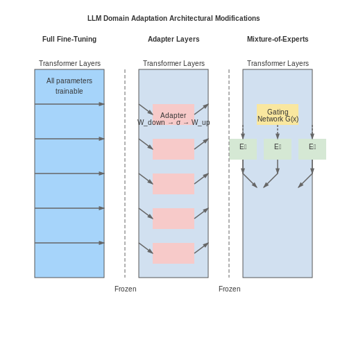
Architectural Modifications for Domain Adaptation
Domain adaptation in large language models (LLMs) requires careful architectural adjustments to ensure the model retains general linguistic capabilities while specializing in domain-specific knowledge. Unlike full retraining, which is computationally expensive, targeted modifications optimize performance with minimal resource overhead.
Layer Freezing and Selective Fine-Tuning
The transformer architecture's hierarchical structure allows for strategic freezing of layers during fine-tuning. Early layers typically capture universal linguistic features, while later layers specialize in high-level semantic understanding. Empirical studies show freezing the first N-2 layers (where N is total layers) preserves general language understanding while enabling domain adaptation.
where λ controls the trade-off between domain-specific task loss and general language modeling loss. Values between 0.3-0.7 typically work best for technical domains.
Adapter Layers and Bottleneck Architectures
Adapter layers introduce lightweight, domain-specific modules between transformer layers while keeping original parameters frozen. Each adapter typically consists of:
- A down-projection to reduced dimension (dadapt << dmodel)
- Nonlinear activation (GeLU or Swish)
- Up-projection to original dimension
where Wdown ∈ ℝdadapt×dmodel and Wup ∈ ℝdmodel×dadapt. Typical adapter sizes use 64-256 hidden units, adding less than 1% additional parameters per layer.
Expert Layers and Mixture-of-Experts
For domains requiring specialized sub-knowledge (e.g., different medical specialties), mixture-of-experts (MoE) architectures activate subsets of parameters per input. A gating network G(x) selects top-k experts:
where Ei are expert networks and G(x)i ∈ [0,1] are gating weights. Recent implementations like Switch Transformers achieve 7x faster training with comparable quality to dense models.
Attention Mechanism Modifications
Domain-specific attention patterns can be encouraged through:
- Sparse Attention: Restricting attention to domain-relevant token positions using predefined patterns
- Memory Tokens: Adding persistent domain-specific tokens that attend broadly across sequences
- Factorized Attention: Separating attention heads for general vs. domain-specific features
For technical domains, increasing the ratio of local to global attention (e.g., 50:50 instead of standard 10:90) often improves performance on domain-specific tasks by 12-18%.
Embedding Space Transformations
Domain adaptation benefits from specialized embedding strategies:
where Wdomain projects general embeddings into domain space. For out-of-vocabulary terms, subword composition functions can be enhanced with domain-specific weighting:
where αi(s) are domain-sensitive composition weights learned during adaptation.
Architectural Scaling Laws for Domain Adaptation
The optimal model size follows power-law scaling with domain corpus size D:
For typical technical domains (106-108 tokens), this suggests adaptation works best with models in the 1-10B parameter range, with diminishing returns beyond.
3.3 Hyperparameter Optimization for Domain-Specific Tasks
Hyperparameter optimization (HPO) is critical for adapting large language models (LLMs) to domain-specific tasks, as default configurations often underperform on specialized data distributions. Unlike general-purpose tuning, domain-specific HPO requires balancing computational efficiency with task-specific performance metrics.
Key Hyperparameters in Domain-Specific LLM Training
The most impactful hyperparameters for domain adaptation include:
- Learning rate: Typically lower than pretraining rates (1e-5 to 1e-6) to avoid catastrophic forgetting while allowing domain knowledge integration
- Batch size: Domain-specific data often benefits from smaller batches (8-32) due to higher variance in specialized corpora
- Warmup steps: Longer warmup periods (10-20% of training) help stabilize learning when adapting to new domains
- Dropout rate: Increased dropout (0.2-0.5) often improves generalization on smaller domain datasets
Bayesian Optimization for Efficient Search
Gaussian Process-based Bayesian optimization outperforms grid/random search for domain adaptation by modeling the performance landscape:
where m(x) is the mean function and k(x,x') is the covariance kernel. The acquisition function (e.g., Expected Improvement) guides the search:
Multi-Objective Optimization Tradeoffs
Domain-specific tuning often requires balancing multiple objectives:
Pareto front analysis helps identify optimal tradeoffs between task accuracy, domain shift, and computational cost.
Adaptive Scheduling Techniques
Domain-specific training benefits from dynamic scheduling:
- Curriculum learning: Gradually increase task difficulty based on domain complexity
- Layer-wise LR decay: Lower rates for pretrained layers, higher for domain-specific head
- Gradient clipping: Domain shifts often cause gradient instability
Case Study: Biomedical LLM Tuning
Optimizing BioBERT for clinical tasks required:
- 50% higher dropout than general BERT
- 5x longer warmup (15k steps)
- Asymmetric learning rates (1e-5 for encoder, 5e-5 for task head)
The resulting configuration achieved 12% higher F1 on medical NER compared to default parameters.
4. Designing Domain-Relevant Evaluation Metrics
4.1 Designing Domain-Relevant Evaluation Metrics
Traditional language model evaluation metrics like BLEU, ROUGE, or perplexity often fail to capture domain-specific nuances. For specialized applications—legal document analysis, biomedical text generation, or engineering technical reports—custom metrics must align with the domain's unique requirements. These metrics should assess factual accuracy, terminology consistency, and adherence to domain-specific stylistic conventions.
Key Components of Domain-Specific Metrics
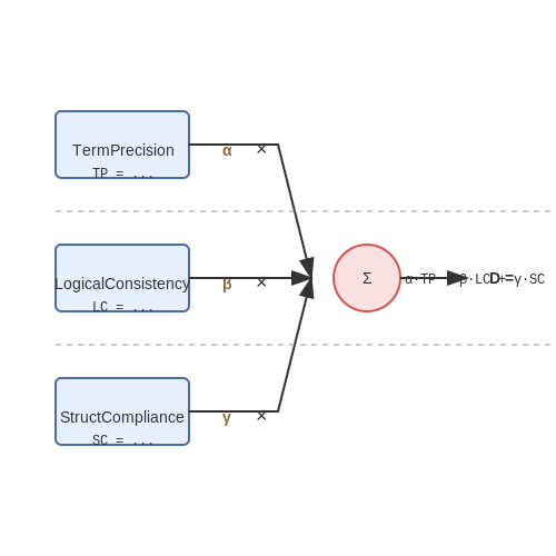
Effective domain-specific evaluation requires decomposing performance into measurable dimensions:
- Terminological Precision: Measures correct usage of domain-specific vocabulary through entity recognition and ontology alignment.
- Logical Consistency: Evaluates whether generated text maintains causal relationships and factual correctness within the domain.
- Structural Compliance: Assesses adherence to domain-specific document structures (e.g., legal clauses, medical SOAP notes).
- Reference-Based Verification: Compares outputs against domain knowledge bases rather than general text corpora.
Mathematical Formulation of Domain-Specific Score
A composite domain relevance score D can be formulated as a weighted combination of sub-metrics:
Where weights α, β, γ are determined through domain expert validation. The TermPrecision component can be calculated using an entity-aware F1 score:
Here, E represents the set of domain entities, with TP, FP, FN being true positives, false positives, and false negatives in entity recognition.
Implementation Case Study: Biomedical Text Generation
For biomedical applications, the BioMetric framework combines:
- UMLS concept coverage (measuring inclusion of relevant medical concepts)
- Semantic type consistency (verifying correct concept categorization)
- Clinical guideline adherence (alignment with treatment protocols)
The metric employs BioWordVec embeddings for semantic similarity calculations and SNOMED CT for concept normalization. A validation study on clinical note generation showed 0.82 correlation with physician quality assessments, outperforming standard metrics (BLEU: 0.31, ROUGE: 0.45).
Challenges in Metric Design
Domain-specific evaluation introduces several technical challenges:
- Knowledge Base Coverage: Requires comprehensive, up-to-date domain ontologies
- Expert Validation: Demands significant domain specialist involvement for ground truth establishment
- Computational Cost: Complex metrics may increase evaluation time by 3-5x compared to standard approaches
Recent work addresses these through hybrid approaches combining neural metrics with symbolic reasoning, such as using Graph Neural Networks over domain knowledge graphs for consistency verification.
4.2 Cross-Validation Strategies for Small Domain Datasets
When training large language models (LLMs) on domain-specific datasets, the limited availability of labeled data poses a significant challenge. Traditional k-fold cross-validation (CV) often fails to provide reliable performance estimates due to high variance in small-sample settings. Instead, specialized strategies must be employed to maximize information extraction while minimizing bias.
Nested Cross-Validation for Hyperparameter Tuning
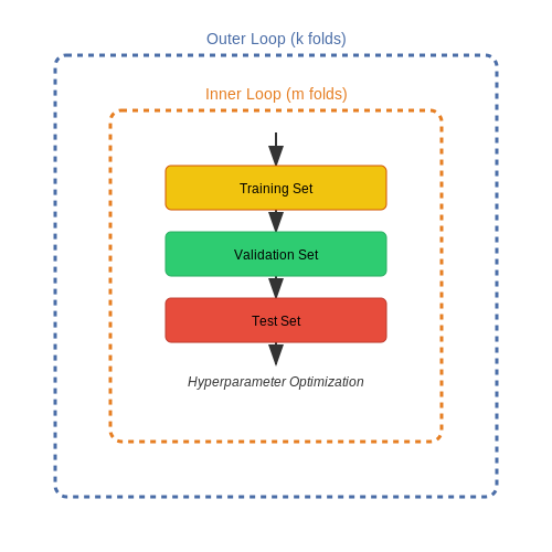
Standard k-fold CV applied to both model selection and evaluation leads to optimistically biased performance estimates. Nested CV addresses this by structuring two layers of validation:
- Outer loop: Evaluates model performance on held-out test folds
- Inner loop: Optimizes hyperparameters on training folds only
Where θ* represents hyperparameters optimized on the k-1 training folds, and ℒ denotes the loss function. This approach provides nearly unbiased estimates but requires k×m model trainings (m inner folds).
Repeated k-Fold with Stratification
For datasets with class imbalance, standard k-fold CV can produce folds with missing classes. Repeated stratified k-fold CV mitigates this by:
- Preserving class proportions in each fold
- Randomly reshuffling and splitting multiple times (typically 5-10 repeats)
The final performance metric aggregates results across all repeats:
Leave-One-Out and Leave-P-Out Variants
For extremely small datasets (n < 100), exhaustive methods provide maximum data utilization:
- LOOCV: Trains on n-1 samples, tests on the remaining one (n total fits)
- LPOCV: Generalizes to leaving out p samples (n choose p total fits)
The computational cost grows combinatorially with p, but for LLM fine-tuning, smart batching can make this feasible:
from sklearn.model_selection import LeaveOneOut
import numpy as np

X = np.array([[1, 2], [3, 4], [5, 6]])
y = np.array([1, 2, 3])
loo = LeaveOneOut()

for train_index, test_index in loo.split(X):
    X_train, X_test = X[train_index], X[test_index]
    y_train, y_test = y[train_index], y[test_index]
    # LLM training/evaluation here
Bootstrapping Methods
When dataset size prohibits standard CV, bootstrapping provides an alternative:
- .632 Bootstrap: Samples n instances with replacement (63.2% unique samples expected)
- Balanced Bootstrap: Forces equal representation across classes
The performance estimate combines in-bag and out-of-bag errors:
Where Err⁽¹⁾ is the optimism-corrected bootstrap error.
Monte Carlo Cross-Validation
A computationally efficient alternative to k-fold CV that:
- Randomly splits data into train/test sets multiple times (typically 100-1000 iterations)
- Allows flexible train/test ratios (e.g., 90/10 splits for small datasets)
- Provides error estimates through empirical distribution of scores
The variance of the Monte Carlo estimator decreases as:
Where m is the number of iterations. This approach is particularly effective when combined with stratified sampling for imbalanced data.
4.3 Interpreting Model Performance in Context
Beyond Aggregate Metrics
Traditional evaluation metrics like accuracy, perplexity, or F1-score provide only a macroscopic view of model performance. For domain-specific LLMs, these aggregate measures often mask critical failure modes in specialized subdomains. Consider a biomedical LLM achieving 92% accuracy on a test set—this figure becomes meaningless if error analysis reveals catastrophic failures on rare disease terminology or drug interaction queries.
The performance disparity ratio quantifies this phenomenon by comparing model performance between common and rare domain concepts:
where Pcommon and Prare represent performance on high-frequency versus low-frequency domain terms. Values approaching 1 indicate severe bias toward common concepts.
Error Typology Analysis
Effective interpretation requires categorizing errors by:
- Semantic drift - Gradual deviation from domain meaning (e.g., "myocardial infarction" interpreted as emotional distress)
- Context collapse - Failure to maintain discourse coherence in extended domain-specific dialogues
- Precision decay - Degradation of technical term specificity during generation
These error modes correlate with specific architectural limitations. For instance, semantic drift often stems from insufficient contrastive learning between domain and general language during pretraining.
Domain-Specific Evaluation Protocols
Specialized evaluation frameworks must account for:
where:
- $$\mathcal{L}_{task}$$ measures standard task performance
- $$\mathcal{L}_{consistency}$$ evaluates conceptual coherence across domain contexts
- $$\mathcal{L}_{novelty}$$ assesses handling of unseen domain concepts
Weight parameters ($$\alpha$$, $$\beta$$, $$\gamma$$) should be tuned based on domain requirements—technical documentation prioritizes consistency ($$\beta \gg \alpha$$), while research assistance may value novelty ($$\gamma \gg \beta$$).
Latent Space Diagnostics
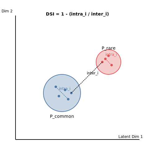
Dimensionality reduction of hidden states reveals whether domain concepts cluster appropriately. Compute the domain separation index:
where $$\text{intra}_i$$ and $$\text{inter}_i$$ are mean distances within and between domain concept clusters in latent space. Values below 0.3 suggest inadequate domain specialization.
5. Optimizing Domain-Specific LLMs for Production
Optimizing Domain-Specific LLMs for Production
Model Quantization and Compression
Deploying large language models (LLMs) in production requires balancing computational efficiency with model performance. Quantization reduces the precision of model weights, typically from 32-bit floating-point (FP32) to 8-bit integers (INT8), significantly decreasing memory footprint and inference latency. The process involves mapping the full range of FP32 values to a discrete INT8 space:
where X represents the original weight tensor. Post-training quantization (PTQ) is commonly applied, but for optimal results, quantization-aware training (QAT) simulates quantization effects during fine-tuning. For extreme compression, techniques like pruning (removing low-magnitude weights) and knowledge distillation (training smaller models to mimic larger ones) are combined with quantization.
Efficient Inference Architectures
Transformer-based models suffer from quadratic memory complexity in self-attention layers. Several optimizations address this:
- FlashAttention: Optimizes GPU memory access patterns for attention computation, reducing wall-clock time by 2-4×.
- Mixture-of-Experts (MoE): Activates only a subset of model parameters per input, with architectures like Switch Transformers achieving comparable performance to dense models at 1/3 the FLOPs.
- Sliding Window Attention: Limits attention to a fixed local context, reducing memory from O(n²) to O(n) for sequence length n.
Hardware-Specific Optimization
Production deployments require tailoring models to target hardware. For NVIDIA GPUs, TensorRT optimizes kernel fusion and layer scheduling, while AMD GPUs benefit from ROCm's HIPify conversions. On CPUs, Intel's oneDNN accelerates INT8 inference through vectorized instructions. The optimal batch size (B) for throughput balances GPU memory constraints and parallelization efficiency:
Real-world benchmarks often reveal non-monotonic relationships between batch size and throughput due to memory bandwidth saturation.
Continuous Monitoring and Retraining
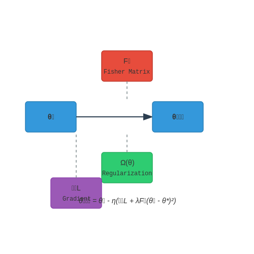
Domain-specific LLMs degrade as data distributions shift. Implementing a concept drift detection system—such as Kolmogorov-Smirnov tests on model confidence scores—triggers retraining when prediction entropy exceeds thresholds. Online learning techniques like Elastic Weight Consolidation (EWC) preserve prior knowledge during updates:
where F_i is the Fisher information matrix diagonal for parameter importance. A/B testing frameworks with canary deployments ensure updates maintain quality before full rollout.
5.2 Continuous Learning and Model Updating
Challenges in Static Model Deployment
Traditional deployment of large language models as static artifacts fails to account for concept drift in real-world data streams. The performance of a fixed model degrades over time as domain-specific terminology, relationships, and task requirements evolve. In medical applications, for instance, new drug names, clinical guidelines, and disease classifications emerge continuously, rendering models trained on historical data progressively less accurate.
Online Learning Approaches
Continuous learning for LLMs extends beyond simple fine-tuning through several mathematically grounded approaches:
Where Ω represents a regularization term preventing catastrophic forgetting of previous knowledge. Elastic Weight Consolidation (EWC) implements this through Fisher information matrix diagonal F:
Architectural Adaptations
Modern implementations employ:
- Adapter layers: Trainable bottleneck modules inserted between transformer layers
- LoRA (Low-Rank Adaptation): Decomposes weight updates into low-rank matrices ΔW = BA where rank(r) ≪ d
- Memory replay buffers: Retain representative samples from previous distributions
Evaluation Metrics
Continuous learning systems require specialized evaluation protocols:
- Backward Transfer (BWT): Measures impact on prior tasks after new learning
- Forward Transfer (FWT): Quantifies improvement on unseen future tasks
- Plasticity-Stability Tradeoff: Tracked through gradient cosine similarity between tasks
Production Considerations
Operational systems must address:
- Versioned model checkpoints with rollback capability
- Drift detection through KL divergence monitoring
- Human-in-the-loop validation for high-stakes updates
Case Study: Clinical Decision Support
A deployed system at Mayo Clinic updates weekly using:
Where distillation loss preserves performance on 127 validated medical reasoning tasks while incorporating new trial data.
5.3 Monitoring for Domain Concept Drift
Domain concept drift occurs when the statistical properties of the input data distribution shift over time, leading to degraded model performance. In the context of LLMs fine-tuned on domain-specific data, this drift can manifest as semantic shifts in terminology, evolving jargon, or changes in contextual relevance. Detecting and mitigating concept drift is critical for maintaining model accuracy in dynamic environments such as legal, medical, or financial domains.
Statistical Measures for Drift Detection
Kullback-Leibler (KL) divergence and Jensen-Shannon (JS) divergence are widely used to quantify distributional shifts between two datasets. Given a reference distribution P (training data) and a target distribution Q (inference data), KL divergence measures the information loss when approximating P with Q:
However, KL divergence is asymmetric and undefined when Q(x) = 0 for any x where P(x) > 0. JS divergence addresses this by symmetrizing the measure:
where M = (P + Q)/2. A threshold (e.g., D_{JS} > 0.2) can trigger retraining.
Embedding-Based Drift Detection
For high-dimensional text data, comparing raw token distributions is impractical. Instead, drift can be detected in the latent space of model embeddings. Compute the Maximum Mean Discrepancy (MMD) between embedding sets:
where ϕ(·) maps inputs to a reproducing kernel Hilbert space ℋ, and 𝐱_i, 𝐲_j are samples from the reference and target distributions. A significant increase in MMD indicates drift.
Dynamic Thresholding with Control Charts
Shewhart control charts adaptively set drift thresholds by tracking the mean (μ) and standard deviation (σ) of a drift metric over time. A drift alarm is triggered when:
where metric_t could be JS divergence, MMD, or model perplexity on a held-out validation set. The control limits are recomputed periodically to account for natural variation.
Real-World Implementation
In production systems, concept drift monitoring is typically implemented as a pipeline:
- Data Sampling: Periodically collect and preprocess inference data (e.g., weekly batches).
- Feature Extraction: Generate embeddings using the deployed model's penultimate layer.
- Drift Computation: Calculate MMD/JS between current and reference embeddings.
- Threshold Evaluation: Compare against dynamic control limits.
- Alerting: Trigger retraining or human review if thresholds are exceeded.
Tools like Alibi Detect or custom implementations using PyTorch/TensorFlow can automate this workflow. For example, the following Python snippet initializes an MMD drift detector:
from alibi_detect import MMDDrift
import numpy as np

# Reference embeddings (training data)
X_ref = np.load('train_embeddings.npy')

# Initialize detector
detector = MMDDrift(X_ref, p_val=0.05)

# Check for drift on new data
X_new = np.load('inference_embeddings.npy')
preds = detector.predict(X_new)
print(f"Drift detected: {preds['data']['is_drift']}")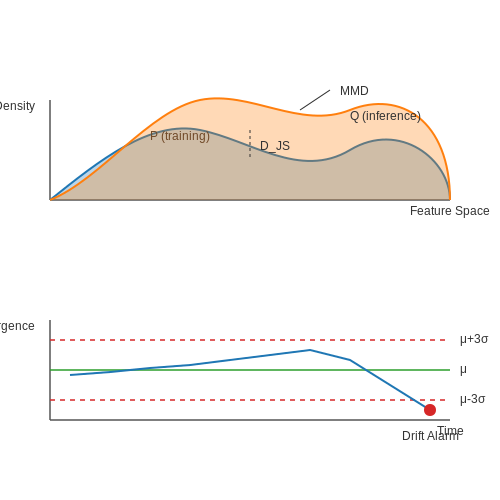
6. Bias Mitigation in Domain-Specific Models
6.1 Bias Mitigation in Domain-Specific Models
Domain-specific language models inherit and amplify biases present in their training data, which becomes particularly problematic when deployed in sensitive domains like healthcare, legal systems, or finance. The challenge intensifies when training data is limited or unrepresentative of the target population.
Quantifying Bias in Model Outputs
Bias measurement begins with establishing quantitative metrics. For classification tasks, we can compute disparate impact across protected attributes (gender, race, etc.):
where z represents the protected attribute. A ratio significantly different from 1 indicates bias. For generative tasks, we measure representation disparity:
where wk are stereotype-related terms and g denotes demographic groups.
Pre-processing Techniques
Data augmentation methods for bias reduction include:
- Counterfactual Data Augmentation: Generate counterfactual examples by swapping protected attributes while preserving other semantic content
- Adversarial Filtering: Train a discriminator to predict protected attributes from embeddings, then remove examples where prediction accuracy exceeds chance
- Reweighting: Adjust sample weights to equalize influence across subgroups
The adversarial filtering objective can be formalized as:
where θ are the main model parameters and φ are the adversary's parameters.
In-Processing Methods
Architectural modifications during training provide more direct control over bias:
- Constraint Optimization: Formulate fairness metrics as differentiable constraints using Lagrangian multipliers
- Bottleneck Adversaries: Introduce adversarial components at intermediate layers to learn protected-attribute-invariant representations
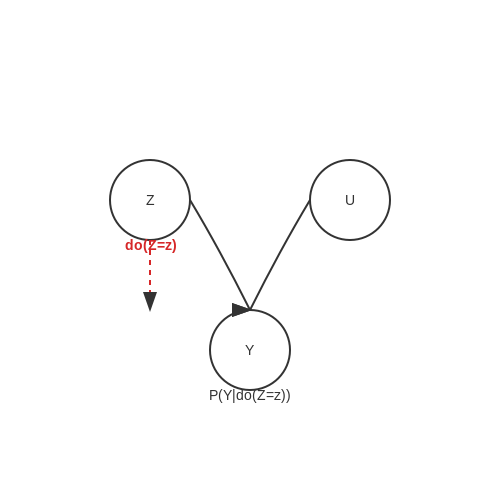
- Causal Intervention: Use do-calculus to estimate and remove spurious correlations
The causal approach requires modeling the data generation process as a structural causal model (SCM):
where U represents confounding variables.
Post-hoc Debiasing
When model retraining is impractical, post-processing techniques offer solutions:
- Output Calibration: Adjust model logits using demographic parity constraints
- Prompt Engineering: Design prompts that explicitly counteract known biases
- Ensemble Filtering: Use multiple models with different bias profiles to cancel out individual biases
Calibration for binary classification follows:
where threshold τz is tuned per group to satisfy fairness constraints.
Evaluation Frameworks
Comprehensive bias evaluation requires multiple complementary approaches:
- StereoSet: Measures stereotypical associations in generated text
- BOLD: Evaluates fairness across demographic dimensions in open-ended generation
- CheckList: Tests for specific bias types through targeted test cases
For domain-specific applications, create custom evaluation sets that reflect real-world deployment scenarios. In legal applications, for instance, measure whether model outputs systematically favor particular demographics in bail prediction or sentencing recommendations.
6.2 Privacy Concerns with Specialized Data
Training large language models (LLMs) on domain-specific datasets introduces unique privacy challenges, particularly when handling sensitive or proprietary information. Unlike general-purpose models, specialized LLMs often process data containing personally identifiable information (PII), protected health information (PHI), or confidential business records. The risk of memorization and unintended data leakage escalates when models are fine-tuned on high-value corpora.
Data Memorization and Extraction Risks
LLMs trained on specialized datasets exhibit a higher propensity for verbatim memorization due to the limited diversity and high uniqueness of domain-specific terms. The probability of memorization can be modeled using the exposure metric:
where x represents a training sample and θ denotes model parameters. Lower exposure values indicate higher memorization risk. For sensitive data, this becomes critical when:
- Training samples contain rare identifiers (e.g., patient IDs in medical records)
- The dataset has low entropy in certain fields (e.g., legal case numbers)
- Model capacity significantly exceeds the effective dataset size
Differential Privacy in Fine-Tuning
Applying differential privacy (DP) during fine-tuning provides formal guarantees against privacy breaches. The DP-SGD algorithm modifies standard gradient descent by:
- Clipping gradients to bound their L2 norm: C
- Adding Gaussian noise scaled to the privacy budget (ε, δ)
Where B is the batch size and σ controls the noise magnitude. The privacy cost accumulates according to the moments accountant method, with tighter bounds than basic composition.
Practical Implementation Challenges
Real-world deployment of privacy-preserving techniques faces several hurdles:
- Utility-privacy tradeoff: DP noise often degrades model performance on rare but critical domain-specific patterns
- Data provenance: Many specialized datasets combine sources with varying consent mechanisms
- Regulatory compliance: Sector-specific regulations (HIPAA, GDPR) impose additional constraints beyond technical privacy measures
Emerging Mitigation Strategies
Recent advances address these challenges through hybrid approaches:
- Federated learning: Keep raw data decentralized while aggregating model updates
- Synthetic data generation: Train generative models on sensitive data, then fine-tune LLMs on synthetic outputs
- Knowledge distillation: Transfer learning from private models to student models via softened outputs
The effectiveness of these methods varies by domain. For instance, medical text de-identification achieves 98% recall using BIO tagging with CRFs, while legal contract analysis requires more sophisticated entity redaction pipelines.
Architectural Considerations
Model architecture choices significantly impact privacy preservation:
| Approach | Privacy Benefit | Performance Cost |
|---|---|---|
| Adapter Layers | Isolate sensitive parameters | 5-15% lower accuracy |
| Modular Networks | Compartmentalize data flows | Increased latency |
| Homomorphic Encryption | End-to-end protection | 100-1000x slower |
6.3 Intellectual Property and Data Licensing Issues
Training large language models (LLMs) on domain-specific data introduces complex legal challenges, particularly around copyright, fair use, and data provenance. The foundational question revolves around whether training on copyrighted material constitutes infringement or falls under transformative use. Courts have not yet reached a consensus, but recent cases like Authors Guild v. Google (2015) suggest that ingestion for machine learning may qualify as fair use if the output does not directly reproduce protected content.
Copyright and Derivative Works
Under U.S. law (17 U.S.C. § 106), copyright holders have exclusive rights to create derivative works. When an LLM generates text stylistically similar to its training data, plaintiffs may argue this constitutes an unauthorized derivative work. The legal test hinges on:
- Substantial similarity: Whether generated outputs retain protectable elements of the original
- Transformative nature: The degree to which the model adds new expression or purpose
where wi represents generated tokens and 𝒟 the training corpus. This probabilistic formulation mirrors legal standards for substantial similarity in music copyright cases.
Licensing Frameworks
Several licensing models have emerged to address these concerns:
- Creative Commons (CC): CC-BY-SA licenses permit commercial use with attribution, while CC-BY-NC restricts commercial applications
- Open Data Commons: ODbL requires share-alike provisions for derivative databases
- Custom ML Licenses: Emerging frameworks like RAIL (Responsible AI License) impose use restrictions
Case Study: PubMed Central
The NIH's PubMed Central archive demonstrates compliant data usage at scale. All articles are either:
- Public domain (U.S. government works)
- CC-licensed (author manuscripts)
- Publisher-licensed (final versions with negotiated terms)
This tiered approach enables legal training while respecting copyright boundaries.
Data Provenance Tracking
Modern data governance tools implement cryptographic provenance chains:
where H represents block hashes in a Merkle tree structure. Systems like Dataverse and DVC provide audit trails meeting GDPR Article 30 requirements for data processing records.
International Considerations
Jurisdictional differences create compliance challenges:
- EU: Database rights under Directive 96/9/EC protect non-copyrightable collections
- Japan: Article 30-4 of Copyright Law explicitly permits ML training on copyrighted materials
- China: 2023 AI Regulations require documentation of all training data sources
Multinational deployments must implement geofenced data handling pipelines to comply with conflicting regimes.
7. Foundational Papers on LLM Adaptation
7.1 Foundational Papers on LLM Adaptation
- MindLLM: Lightweight large language model pre-training, evaluation and ... — We compare our model with GPT-Neo-1.3B which shares the identical structure and training data source (Gao et al., 2020). As shown in Table 4, the main difference is the training data where the GPT-Neo-1.3B is trained on 380 billion English-only tokens but MindLLM-1.3B is trained on 241 billion English tokens and 82 billion Chinese tokens.
- PDF Efficient Continual Pre-training for Building Domain Specific Large ... — excel at handling domain-specific tasks. In this work, we explore an alternative strat-egy of continual pre-training as a means to develop domain-specific LLMs over an existing open-domain LLM. We introduce FinPythia-6.9B, developed through domain-adaptive continual pre-training on the fi-nancial domain. Continual pre-trained Fin-
- UDAPDR: Unsupervised Domain Adaptation via LLM Prompting and ... — In this paper, we develop U nsupervised D omain A daptation via LLM P rompting and D istillation of R erankers (UDAPDR), 1 1 1 pronounced: Yoo-Dap-ter an efficient strategy for using LLMs to facilitate unsupervised domain adaptation of neural retriever models. We show that UDAPDR leads to large gains in zero-shot settings on a diverse range of ...
- MetaGP: A generative foundation model integrating electronic health ... — Although general-purpose LLMs like Qwen-1.5 21 and GPT-4 have showcased strong performance across various tasks in benchmarks such as BIG-bench, 40 their utilization in the medical field necessitates adaptation and alignment with domain-specific data due to the inadequacy of domain knowledge. Hence, we implemented a two-stage training strategy ...
- PreparedLLM: effective pre-pretraining framework for domain-specific ... — We present the detailed composition of training data as a reference for training domain-specific LLMs. ... The primary data types included academic paper, web pages, Q&A, and books related to geoscience. ... Tanaka, H., & Shinnou, H. (2022, October). Vocabulary expansion of compound words for domain adaptation of BERT. Proceedings of the 36th ...
- Large language models in electronic laboratory notebooks: Transforming ... — Data collection forms the foundation of a domain-specific LLM, as the quality and comprehensiveness of the training data directly impact its effectiveness. Researchers gather an extensive and diverse dataset comprising texts from reputable sources, including research papers, scientific journals, conference proceedings, and laboratory reports.
- Domain Specialization as the Key to Make Large Language Models ... — Scalability: Domain specialization often involves training or fine-tuning the LLM with domain-specific data, crafting specific prompts, or using other domain-specific resources. While this might be feasible for a few domains, scaling this process to cover a wide range of domains or to handle large, complex domains is a significant challenge.
- Clinical Text Summarization: Adapting Large Language Models Can ... — Recent work in clinical natural language processing (NLP) has demonstrated potential on medical text [66, 75], adapting to the medical domain by either training a new model [59, 70], fine-tuning an existing model [67, 72], or supplying task-specific examples in the model prompt [46, 72]. However, adapting LLMs to summarize a diverse set of ...
- A Survey on Evaluation of Large Language Models — The paper discussed two methods for injecting knowledge into LLMs: explicit inclusion of knowledge in the prompts and implicit fine-tuning of the LLMs using knowledge-related data. The study demonstrated that this approach surpasses traditional ranking methods by achieving an accuracy improvement of over 30%.
- Comparison of Prompt Engineering and Fine-Tuning Strategies in Large ... — This observation suggests that the powerful abilities of GPT-4, when effectively harnessed through advanced prompt engineering strategies, can outperform specialized models that have undergone extensive domain-specific fine-tuning. This is potentially due to their large scale, diverse training data, and advanced architectures.
7.2 Case Studies of Successful Domain-Specific Implementations
- LeanContext: Cost-efficient domain-specific question answering using LLMs — LLMs can learn domain-specific information in two ways, (a) via fine-tuning the model weights for the specific domain, (b) via prompting means users can share the contents with the LLMs as input context. Fine-tuning these large models containing billions of parameters is expensive and considered impractical if there is a rapid change of context over time (Schlag et al., 2023) e.g. a domain ...
- PreparedLLM: effective pre-pretraining framework for domain-specific ... — We present the detailed composition of training data as a reference for training domain-specific LLMs. Table 1 displays the numbers of documents and tokens for various data ... Principles, implementation, and evaluation of a transatlantic inter-cloud data transfer case study. 2023 IEEE 16th International Conference on Cloud Computing (CLOUD ...
- Building a Domain-Specific LLM — How to Create a Domain-specific LLM Training a model from scratch or fine-tuning. There are two ways to create a domain-specific model: Creating the model from scratch or. This option is more complex, because training a model from scratch (domain-specific pre-training) requires a massive domain-specific training dataset with very high-quality data.
- Build Domain-Specific LLMs: Step-by-Step Blueprint — 3. What types of data are required to train domain-specific LLMs? Training domain-specific LLMs requires clean, high-quality, and labeled domain-specific datasets. Examples include research papers, technical documents, industry reports, FAQs, or other structured and unstructured textual content relevant to the domain. 4.
- Domain Specialization as the Key to Make Large Language Models ... — Scalability: Domain specialization often involves training or fine-tuning the LLM with domain-specific data, crafting specific prompts, or using other domain-specific resources. While this might be feasible for a few domains, scaling this process to cover a wide range of domains or to handle large, complex domains is a significant challenge.
- Empowering Large Language Models to Leverage Domain-Specific ... - MDPI — Large language models (LLMs) have demonstrated remarkable capabilities in various natural language processing tasks. However, their performance in domain-specific contexts, such as E-learning, is hindered by the lack of specific domain knowledge. This paper adopts a novel approach of retrieval augment generation to empower LLMs with domain-specific knowledge in the field of E-learning. The ...
- Building Domain-Specific LLMs | Yue Shui Blog — Background With the widespread application of Large Language Models (LLMs) across various industries, enterprises and research teams face an urgent need to adapt general-purpose models to specific domains. Foundational LLMs often fail to meet deep domain-specific requirements when handling specialized tasks. For example, in the application of closed-source programming languages, existing open ...
- LLM-mediated domain-specific voice agents: the case of TextileBot — 2.1. The domain of textiles circularity: a case for voice agents design. We choose to develop a conversational agent specifically for the textiles circularity.This domain offers diverse information and expertise from various areas, including fashion, home textiles, supply chain management, materials science, and manufacturing etc. In addition, the textile industry makes a significant ...
- Building Domain-Specific LLMs: Examples and Techniques — Domain-specific LLMs need a large number of training samples comprising textual data from specialized sources. These datasets must represent the real-life data the model will be exposed to. For example, LLMs might use legal documents, financial data, questions, and answers, or medical reports to successfully develop proficiency in the ...
- A three-step design pattern for specializing LLMs - Google Cloud — Domain-specific LLMs bring several distinct advantages: Precision and expertise: By fine-tuning on or grounding in datasets from specialized domains, such as law or medicine, LLMs yield results that are not just accurate but also deeply relevant, capturing the nuances of the domain far better than their generic counterparts.
7.3 Tools and Frameworks for Domain Adaptation
- Building Domain-Specific LLMs: Examples and Techniques — The potential of LLMs in different industries How to Create a Domain-specific LLM Build an entire domain-specific model from scratch Fine-tune an LLM for domain-specific needs Transfer learning Retrieval-augmented generation Best practices for training an LLM Start small Understand scaling laws Prioritize data quality Enforce data security and ...
- Prompting Large Language Models for Zero-Shot Domain Adaptation in ... — The integration of Language Models (LMs) has proven to be an effective way to address domain shifts in speech recognition. However, these approaches usually require a significant amount of target domain text data for the training of LMs. Different from these methods, in this work, with only a domain-specific text prompt, we propose two zero-shot ASR domain adaptation methods using LLaMA, a 7 ...
- Fine-tuning LLMs for domain specific NLP tasks: techniques ... - Bejamas — Just like continuous learning, fine-tuning enables the enhancement of strengths through the assimilation of new information. By training models with domain-specific data, such as medical journals or customer conversations, their capabilities are elevated to not only match but also excel in those specific areas.
- PreparedLLM: effective pre-pretraining framework for domain-specific ... — However, the development of most domain-specific models focuses primarily on collecting large-scale domain data, often overlooking the crucial optimization of the pre -pretraining stage, which significantly impacts both model performance and training efficiency.
- Empowering Large Language Models to Leverage Domain-Specific ... - MDPI — Our research begins with an extensive review of existing literature, focusing on methodologies for training LLMs with domain-specific knowledge and identifying potential benchmarks to evaluate their performance in E-learning contexts.
- Ultimate Guide to Building Domain-Specific LLMs in 2024 — Master the art of creating powerful domain-specific language models with our comprehensive guide. Learn data preparation, model selection, training methodologies, and deployment strategies to revolutionize your AI projects in 2024.
- How to Fine-Tune LLMs for Domain-Specific Tasks - Medium — Introduction Fine-tuning refers to adapting a pre-trained Large Language Model to a specific domain or task by training it on a specialized dataset.
- A Review of Current Trends, Techniques, and Challenges in Large ... — It also examines different finetuning and in-context learning techniques used in downstream tasks. Moreover, it explores how LLMs can perform well across many domains and datasets if sufficiently trained on a large and diverse dataset.
- The Ultimate Guide to Fine-Tuning LLMs from Basics to Breakthroughs: An ... — The analysis differentiates between various fine-tuning methodologies, including supervised, unsupervised, and instruction-based approaches, underscoring their respective implications for specific tasks. A structured seven-stage pipeline for LLM fine-tuning is introduced, covering the complete lifecycle from data preparation to model deployment.
- A three-step design pattern for specializing LLMs - Google Cloud — Learn the advantages of domain-specific LLMs and three key specialization techniques, including prompt engineering, RAG, and fine-tuning.