AI That Understands Other AI Outputs
1. Defining AI Interpretation and Meta-Understanding
Defining AI Interpretation and Meta-Understanding
AI interpretation refers to the ability of an artificial intelligence system to analyze, explain, or contextualize the outputs generated by another AI model. This involves not just parsing raw predictions or classifications but also inferring the underlying reasoning, uncertainty, or latent representations that produced them. Meta-understanding extends this further by enabling an AI to model the internal states, knowledge boundaries, or decision-making processes of other AI systems.
Formalizing Interpretation as a Learning Problem
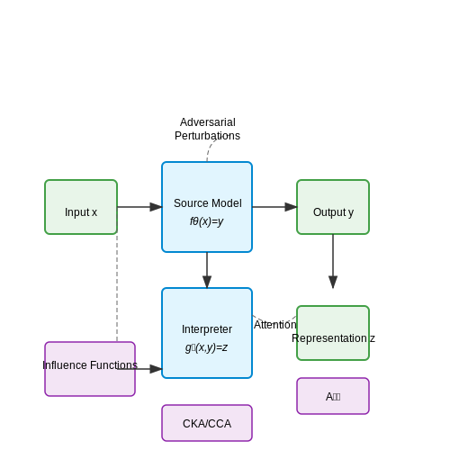
Given a source model fθ and its output y = fθ(x), an interpreter model gϕ aims to learn a mapping:
where z represents an interpretable representation—such as feature attributions, concept activations, or symbolic explanations. For differentiable models, this can be framed as optimizing:
with z* being ground-truth explanations when available, ℒ a suitable loss function (e.g., KL divergence for probabilistic explanations), and R a regularization term enforcing desired properties like sparsity.
Meta-Understanding Through Model Probing
Advanced interpretation requires going beyond post-hoc analysis to actively probe the source model's behavior. Techniques include:
- Adversarial Perturbation Analysis: Systematically varying inputs to identify decision boundaries and vulnerable features.
- Representation Similarity Metrics: Comparing latent space geometries using centered kernel alignment (CKA) or canonical correlation analysis (CCA).
- Influence Functions: Estimating how training points affect predictions via:
where Hθ is the Hessian of the source model's loss.
Architectural Considerations
Effective interpreter models often employ hybrid architectures:
- Cross-Modal Attention: Aligns tokens or features between the source model's internal representations and human-interpretable concepts.
- Memory-Augmented Networks: External memory banks store prototypical explanations for retrieval and adaptation.
- Recursive Reasoning Modules: Explicitly model the source AI's potential chain-of-thought through iterative refinement.
Case Study: Interpreting Vision Transformers
For a Vision Transformer (ViT), meta-understanding involves:
where Al,h is the attention matrix for layer l and head h, followed by concept activation vectors (CAVs) learned via logistic regression on annotated concept datasets.
Key Challenges in AI Output Comprehension
Semantic Ambiguity in Model Outputs
Modern AI systems, particularly large language models (LLMs), generate outputs that are syntactically coherent but often semantically ambiguous. This arises from the probabilistic nature of token prediction, where multiple valid interpretations may exist for a given output. For instance, an LLM-generated statement like "The patient responded well to the treatment" could imply either clinical improvement or mere compliance with medication.
where wt represents the token at position t, and the conditional probability distribution inherently contains multiple high-probability paths.
Lack of Explainable Intermediate Representations
Neural architectures process information through high-dimensional latent spaces that lack human-interpretable semantics. While attention mechanisms in transformers provide some visibility into input-output relationships, the emergent representations in deeper layers remain opaque. This creates a fundamental disconnect between the model's internal reasoning and human-understandable explanations.
Distributional Shift Between Training and Deployment
When AI systems encounter inputs outside their training distribution, their outputs become unreliable yet often maintain surface-level plausibility. The epistemic uncertainty in these cases is rarely communicated effectively. For a model trained on medical literature analyzing patient-generated text:
where the KL divergence between training and deployment distributions exceeds acceptable thresholds.
Compositional Generalization Limits
Current architectures struggle with systematic composition of learned concepts. When processing novel combinations of known elements, models frequently generate outputs that appear correct locally but are globally inconsistent. This manifests particularly in:
- Logical reasoning tasks requiring multi-step inference
- Counterfactual scenario analysis
- Cross-domain knowledge transfer
Temporal Coherence in Sequential Outputs
Maintaining consistent state representations across long sequences remains challenging. In dialogue systems or multi-step reasoning tasks, models exhibit:
- Entity drift (gradual alteration of referenced objects)
- Predicate contradiction
- Temporal inconsistency in event ordering
The hidden state update mechanism in recurrent architectures:
progressively loses precision over long sequences due to information compression.
Multimodal Alignment Challenges
When processing inputs or generating outputs across multiple modalities (text, image, audio), current systems often fail to maintain semantically consistent cross-modal references. The alignment loss between modalities i and j:
where φ represents modality-specific encoders, frequently remains non-zero even in state-of-the-art multimodal systems.
Role of Explainability and Transparency
Explainability and transparency are critical for enabling AI systems to interpret and understand the outputs of other AI models. Without these properties, the interactions between models become opaque, leading to potential misalignment, adversarial vulnerabilities, and unreliable decision-making. Explainability refers to the ability of a model to provide human-understandable justifications for its outputs, while transparency ensures that the internal mechanisms and data flows are accessible for inspection.
Mathematical Foundations of Explainability
Explainability in AI can be formalized using interpretability metrics, such as feature importance scores or Shapley values. For a given model f and input x, the Shapley value ϕ_i for feature i is computed as:
where N is the set of all features, and S is a subset of features excluding i. This formulation ensures a fair attribution of each feature's contribution to the model's output, enabling interpretability.
Transparency in Model Architectures
Transparency is achieved through architectural choices that expose intermediate computations. For instance, attention mechanisms in transformer models provide a natural form of transparency by revealing which input tokens influence specific outputs. The attention weight α_{ij} between token i and token j is given by:
where e_{ij} is the scaled dot-product similarity between the query and key vectors. Visualizing these weights allows practitioners to trace how information propagates through the model.
Practical Applications
In multi-agent AI systems, explainability and transparency enable models to critique and refine each other's outputs. For example, a diagnostic AI might generate a preliminary assessment, while a secondary model evaluates the reasoning behind this assessment using saliency maps or counterfactual explanations. This iterative process improves robustness and reduces the risk of cascading errors.
Another application is in federated learning, where transparency ensures that local model updates can be audited for consistency before aggregation. Techniques like differential privacy and secure multi-party computation can be combined with explainability methods to maintain privacy while allowing meaningful interpretation of contributions from participating models.
Challenges and Trade-offs
While explainability and transparency are desirable, they often come at the cost of computational overhead or reduced model performance. For instance, simpler interpretable models like decision trees may underperform compared to deep neural networks on complex tasks. Additionally, adversarial attacks can exploit transparency by reverse-engineering model behavior, necessitating a careful balance between openness and security.
2. Model-Agnostic Interpretation Methods
Model-Agnostic Interpretation Methods
Model-agnostic interpretation techniques provide insights into any machine learning model's behavior without requiring access to its internal parameters or architecture. These methods treat the model as a black box, relying solely on input-output interactions to derive explanations. Their flexibility makes them indispensable for interpreting complex ensembles, deep neural networks, or proprietary systems where internal workings are opaque.
Local Interpretable Model-agnostic Explanations (LIME)
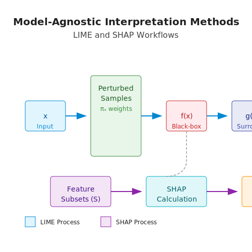
LIME approximates complex models locally with interpretable surrogate models (e.g., linear classifiers or decision trees). Given an input instance x, LIME generates perturbed samples around x, queries the black-box model for predictions, and fits a weighted interpretable model to these samples. The explanation is derived from the surrogate model's coefficients.
where f is the black-box model, g the interpretable model, πx a proximity measure, and Ω(g) a complexity penalty. The loss ℒ ensures fidelity to f's predictions in the neighborhood of x.
SHAP (SHapley Additive exPlanations)
SHAP values provide a game-theoretic approach to feature attribution by computing each feature's marginal contribution across all possible coalitions. For a model f and instance x, the SHAP value ϕi for feature i is:
where F is the set of all features, and fS denotes the model's prediction conditioned on feature subset S. SHAP values satisfy efficiency (summing to the prediction output) and symmetry (equal contributions for equally influential features).
Partial Dependence Plots (PDP)
PDPs visualize the marginal effect of one or two features on predictions by averaging over other features' distributions. For feature subset S and complement C, the partial dependence function is:
Individual Conditional Expectation (ICE) plots extend PDPs by showing prediction trajectories for individual instances, revealing heterogeneity in feature effects.
Global Surrogate Models
These methods train an interpretable model (e.g., decision tree, logistic regression) to mimic a black-box model's global behavior. The surrogate's structure provides insights into the original model's decision logic. Performance metrics (e.g., R², accuracy) quantify how well the surrogate approximates the black box.
Practical Considerations
- Feature perturbations in LIME/SHAP must respect data manifolds to avoid unrealistic samples.
- Computational cost grows exponentially with feature count for exact SHAP calculations; kernel-based approximations are often used.
- Explanation fidelity depends on surrogate model complexity and local approximation quality.
2.2 Neural Network-Based Interpreters
Neural network-based interpreters leverage deep learning architectures to decode and interpret the outputs of other AI models, particularly black-box systems where traditional explainability methods fall short. These interpreters are trained to map complex, high-dimensional model outputs (e.g., activations, attention weights, or latent representations) to human-understandable explanations or lower-dimensional semantic spaces.
Architectural Foundations
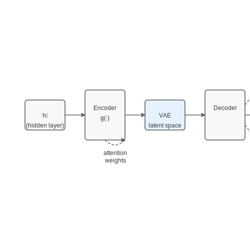
The core architecture typically consists of an encoder-decoder framework, where the encoder processes the target model's internal states, and the decoder generates interpretable outputs. For instance, given a neural network f with hidden layer activations hl, an interpreter g learns a mapping:
where ϕ is an interpretable representation (e.g., feature importance scores or natural language descriptions). Variants include:
- Attention-based interpreters: Use cross-attention mechanisms to align target model activations with interpretable tokens or concepts.
- Variational autoencoder (VAE) interpreters: Project activations into a latent space where dimensions correspond to semantically meaningful factors.
- Graph neural network (GNN) interpreters: Model relationships between neurons or layers as a graph, enabling structural explanations.
Training Paradigms
Training neural interpreters requires carefully designed loss functions to balance fidelity (accuracy in reconstructing the target model's behavior) and interpretability. A common approach combines:
where ℒfidelity measures output reconstruction error (e.g., mean squared error for regression tasks or cross-entropy for classification), and ℒsimplicity enforces sparsity or low-dimensionality constraints. For example, in attention-based interpreters, ℒsimplicity may penalize entropy in attention distributions to encourage focused explanations.
Case Study: Interpreting Vision Transformers
To interpret a Vision Transformer (ViT), a neural interpreter might process the model's patch embeddings and self-attention weights. The encoder could be a convolutional network that aggregates spatial information, while the decoder generates heatmaps highlighting influential image regions. The training objective would include:
where y(i) are ground-truth segmentation masks or human-annotated saliency maps. The interpreter's output can then be validated using metrics like pointing game accuracy or area-under-the-curve (AUC) for localization tasks.
Limitations and Trade-offs
While powerful, neural interpreters introduce their own opacity—the interpreter itself becomes a secondary black box. Techniques like iterative distillation or adversarial validation are used to ensure the interpreter's explanations remain faithful to the target model's decision boundaries. Additionally, computational overhead scales with the complexity of the target model, making real-time interpretation challenging for large-scale architectures like GPT-4 or Claude 3.
2.3 Knowledge Distillation for Cross-Model Understanding
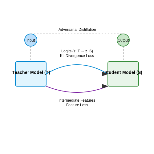
Knowledge distillation (KD) enables a smaller student model to mimic the behavior of a larger teacher model by transferring learned representations, typically through soft target probabilities. The core objective is to compress knowledge from a complex model into a more efficient one while preserving predictive performance. For cross-model understanding, KD extends beyond compression—it facilitates interpretability and interoperability between heterogeneous architectures.
Formalizing Knowledge Distillation
The standard KD loss function combines a student's prediction error on ground-truth labels with a distillation loss that aligns the student's softened outputs with the teacher's. Given a teacher model T and student model S, the total loss is:
where zT and zS are logits from teacher and student, σ is the softmax function, τ is the temperature parameter controlling output smoothness, and λ balances the two losses. The Kullback-Leibler (KL) divergence term forces the student to learn the teacher's relative class relationships, which often contain implicit dark knowledge not present in hard labels.
Cross-Architecture Distillation Challenges
When teacher and student models have fundamentally different architectures (e.g., CNN to Transformer), direct logit matching becomes suboptimal. Three key adaptations address this:
- Intermediate Representation Alignment: Minimizes distance between hidden layer activations using techniques like attention transfer or Gram matrix matching.
- Dynamic Temperature Scaling: Adjusts τ during training to handle varying output scale disparities between architectures.
- Adversarial Distillation: Uses a discriminator network to ensure the student's feature distributions are indistinguishable from the teacher's.
Practical Implementation
For a CNN-to-Transformer distillation task, the following PyTorch snippet demonstrates intermediate feature matching:
def feature_loss(teacher_feats, student_feats):
   # L2 distance on normalized features
   return F.mse_loss(
      F.normalize(teacher_feats, p=2, dim=1),
      F.normalize(student_feats, p=2, dim=1)
   )

# Training loop excerpt
for inputs, labels in dataloader:
   teacher_logits, t_feats = teacher(inputs, return_features=True)
   student_logits, s_feats = student(inputs, return_features=True)

   loss = (0.7 * F.cross_entropy(student_logits, labels)
          + 0.3 * feature_loss(t_feats[-3], s_feats[-3])  # Match penultimate layer
   loss.backward()
Emerging Research Directions
Recent advances focus on multi-modal distillation, where a teacher's cross-modal understanding (e.g., vision-language models) is transferred to unimodal students. Techniques like cross-modal attention distillation show promise in preserving relational knowledge between modalities. Another frontier is self-distillation, where a single model serves as both teacher and student through iterative refinement.
Attention Mechanisms for Output Analysis
Attention mechanisms enable AI models to dynamically focus on relevant parts of another AI's output, improving interpretability and downstream task performance. The core idea stems from the human cognitive process of selectively concentrating on salient information while filtering out noise. In transformer architectures, attention is computed as a weighted sum of values, where weights are derived from the compatibility between queries and keys.
Scaled Dot-Product Attention
The fundamental operation in attention mechanisms is scaled dot-product attention, defined as:
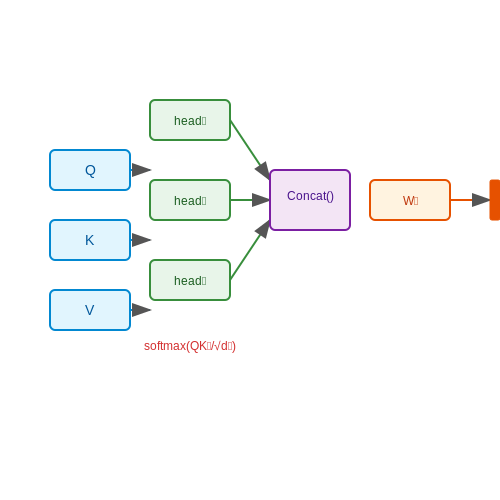
where Q, K, and V represent queries, keys, and values matrices respectively, and dk is the dimension of the keys. The scaling factor 1/√dk prevents gradients from becoming too small when dk is large.
Multi-Head Attention
Multi-head attention extends this by applying the attention mechanism in parallel across h different learned linear projections:
where each head is computed as:
The projection matrices WiQ, WiK, WiV and WO are learnable parameters. This allows the model to jointly attend to information from different representation subspaces.
Cross-Attention for AI Output Understanding
When analyzing another AI's outputs, cross-attention becomes particularly useful. Here, the queries come from one model while the keys and values come from another:
This mechanism enables the analyzing model to dynamically retrieve relevant information from the source model's outputs. The attention weights can be interpreted as the analyzing model's "focus" on different parts of the source output.
Practical Implementation Considerations
For efficient implementation of attention mechanisms in output analysis tasks:
- Memory optimization: Use flash attention for long sequences to reduce memory footprint
- Sparse attention: Implement localized or pattern-based attention for computational efficiency
- Attention masking: Apply causal or padding masks as needed for the specific task
- Gradient flow: Monitor attention weight gradients to ensure stable training
The attention mechanism's output can be further processed through feed-forward networks and layer normalization, following standard transformer architecture practices. Recent advances like Perceiver IO demonstrate how attention can effectively process outputs from diverse AI systems by treating them as byte arrays with learned positional embeddings.
3. AI Auditing and Debugging Systems
AI Auditing and Debugging Systems
Formal Verification of Neural Networks
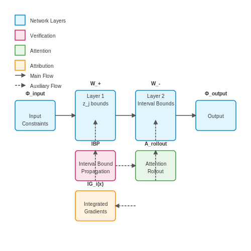
Formal verification techniques provide mathematical guarantees about neural network behavior by framing properties as constraints solvable via satisfiability modulo theories (SMT). Given a neural network f with weights W and inputs x, we can express output constraints as:
where Φinput defines valid input ranges and Φoutput specifies safety conditions. Reluplex extends simplex algorithms to handle ReLU activation functions by introducing slack variables s for each neuron:
Gradient-Based Attribution Methods
Integrated Gradients attribute model decisions to input features by accumulating gradients along the path from baseline x' to input x:
Shapley values from cooperative game theory provide theoretically optimal feature attribution by evaluating all possible feature coalitions:
Adversarial Robustness Certification
Interval bound propagation (IBP) computes guaranteed output bounds under input perturbations δ by propagating interval arithmetic through layers:
where W+ and W- denote positive/negative weight components. For convolutional networks, Fourier-domain certifications provide tighter bounds by exploiting convolution theorem:
Interpretability Through Architectural Inductive Biases
Neural additive models enforce interpretability through additive structure:
where each gi is a shallow network processing only the i-th feature. Attention rollout matrices in transformers reveal cross-layer token dependencies:
where A(l) are attention matrices at layer l and I is the identity matrix.
Debugging via Latent Space Probing
Probing classifiers trained on hidden representations quantify learned concepts through linear separability:
where hi are hidden states and yi concept labels. Counterfactual explanations identify minimal input changes altering model decisions by solving:
using gradient-based optimization or genetic algorithms for non-differentiable models.
3.2 Collaborative Multi-Agent Systems
In multi-agent reinforcement learning (MARL), agents must not only optimize their own policies but also interpret and respond to the actions of other agents. This requires a shared understanding of the environment and other agents' strategies. A key mathematical framework for this is the Nash equilibrium, where no agent can improve its reward by unilaterally changing its policy. For a set of agents with policies \(\pi_1, \pi_2, \dots, \pi_N\), the Nash equilibrium satisfies:
Here, \(V_i\) represents the value function for agent \(i\), and \(\pi_{-i}^*\) denotes the optimal policies of all other agents. Achieving this equilibrium in practice often requires decentralized training with centralized execution (DTCE), where agents learn independently but coordinate during deployment.
Communication Protocols in Multi-Agent Systems
Agents can exchange information via learned communication protocols, often modeled as differentiable channels. A common approach is to use attention mechanisms to weigh the importance of messages from other agents. The message aggregation for agent \(i\) can be expressed as:
where \(\alpha_{ij}\) is the attention weight, and \(\phi_j\) is a learned message function. The weights are computed using a softmax over a compatibility score:
Here, \(f\) is a compatibility function, often implemented as a dot product between transformed states.
Emergent Behaviors in Multi-Agent Systems
Complex cooperative strategies can emerge from simple local interactions. For example, in predator-prey simulations, agents may develop flanking maneuvers without explicit programming. This is formalized using mean-field theory, where the effect of other agents is approximated by a mean field:
where \(\bar{a}\) represents the average action of neighboring agents. This approximation reduces computational complexity while preserving emergent coordination.
Applications in Real-World Systems
Collaborative multi-agent systems are deployed in:
- Autonomous vehicle coordination: Agents negotiate lane changes and merges using game-theoretic principles.
- Warehouse robotics: Multi-agent pathfinding algorithms minimize congestion while maximizing throughput.
- Smart grid management: Agents representing energy producers and consumers balance supply and demand through distributed optimization.
Recent advances in graph neural networks have enabled agents to reason about relational structures in their environment, further improving collaborative decision-making. The adjacency matrix \(A\) encodes agent connectivity, and graph convolutions propagate information:
where \(D\) is the degree matrix, \(H^{(l)}\) contains node features at layer \(l\), and \(W^{(l)}\) are learnable weights.
3.3 AI-Generated Content Verification
Modern AI systems, particularly large language models (LLMs) and generative adversarial networks (GANs), produce outputs that are increasingly indistinguishable from human-generated content. This necessitates robust verification mechanisms to ensure authenticity, correctness, and ethical compliance. Verification techniques can be broadly categorized into statistical, semantic, and adversarial methods.
Statistical Verification
Statistical methods analyze the probability distributions of generated outputs to detect anomalies. Given a generative model G with output x, the likelihood score L(x) is computed as:
where PG(x) is the probability of x under the model. Low-likelihood outputs may indicate synthetic generation. However, this approach is limited by the model's own biases and may fail for high-quality adversarial samples.
Semantic Verification
Semantic verification evaluates logical consistency and factual accuracy. For text, entailment models compute:
where C(x) is a set of claims extracted from x. For images, semantic segmentation inconsistencies can reveal synthetic origins. State-of-the-art methods use cross-modal verification, where text descriptions are compared against generated images for coherence.
Adversarial Verification
Adversarial verification employs auxiliary models trained to discriminate between human and AI-generated content. The discriminator D is optimized via:
Recent advancements incorporate self-supervised learning, where verification models are trained on contrastive objectives to distinguish real and synthetic data without explicit labels.
Case Study: Detecting GPT-4 Outputs
OpenAI's GPT-4 detector combines statistical and semantic methods by analyzing:
- Perplexity scores relative to human text distributions
- Factual consistency via knowledge graph embeddings
- Stylometric patterns (e.g., repetition frequency, syntactic complexity)
Empirical results show 92% accuracy on curated datasets, though performance degrades with human-AI collaborative writing.
Challenges and Future Directions
Current verification systems struggle with:
- Generalization: Detectors trained on one model (e.g., GPT-3) often fail on newer versions (e.g., GPT-4)
- Adaptive adversaries: Generative models can be fine-tuned to evade specific detectors
- Multimodal consistency: Verifying cross-modal outputs (e.g., text+image) remains unsolved
Emerging solutions include watermarking via imperceptible perturbations in latent spaces and provenance tracking using cryptographic signatures embedded during generation.
4. Bias Propagation in AI-to-AI Understanding
4.1 Bias Propagation in AI-to-AI Understanding
When one AI system interprets the outputs of another, biases present in the first model can propagate and amplify through the interaction. This phenomenon occurs due to the compounding of statistical dependencies, architectural constraints, and training data limitations across multiple AI systems. The propagation of bias is not merely additive; nonlinear interactions between models can lead to emergent biases that were not explicitly present in either system individually.
Mathematical Formulation of Bias Propagation
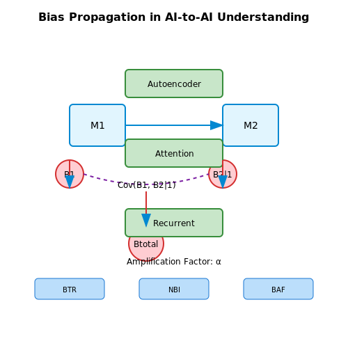
Consider two AI models, M1 and M2, where M2 processes the outputs of M1. Let B1 represent the bias in M1's predictions, and B2|1 represent the conditional bias introduced by M2 when interpreting M1's outputs. The total bias Btotal can be modeled as:
where the covariance term captures the interaction between the biases of the two models. When M2 is trained on outputs from M1, the expectation term becomes:
with p1(y) being the output distribution of M1. This integral shows how M1's bias directly influences the learned behavior of M2.
Architectural Amplification Mechanisms
Certain neural architectures are particularly prone to bias amplification:
- Autoencoder-based systems tend to reinforce latent space biases through reconstruction losses
- Attention mechanisms can disproportionately focus on biased features from the input model
- Recurrent connections allow bias to accumulate across sequential processing steps
The amplification factor α for a given architectural component can be quantified through the Jacobian of the component's transformation:
where f(x) represents the component's operation and μ is the mean input.
Empirical Measurement Approaches
Several metrics have been developed to quantify bias propagation in AI systems:
- Bias Transfer Ratio (BTR): Measures the fraction of input bias that appears in the output
- Novel Bias Introduction (NBI): Quantifies new biases introduced by the interpreting model
- Bias Amplification Factor (BAF): Computes the ratio of output bias magnitude to input bias magnitude
For a pair of models M1 → M2, the BAF is calculated as:
Values greater than 1 indicate amplification, while values less than 1 suggest attenuation of bias.
Mitigation Strategies
Effective approaches to reduce bias propagation include:
- Adversarial debiasing: Training the interpreting model with an adversarial objective to remove dependencies on biased features
- Causal intervention: Modifying the interpretation process to break spurious correlations
- Multi-model verification: Using ensemble methods to detect and correct biased interpretations
The adversarial debiasing approach modifies the loss function to include a term that penalizes the ability to predict protected attributes:
where λ controls the strength of debiasing.
4.2 Security Risks and Adversarial Manipulation
Adversarial Attacks on AI Interpretability
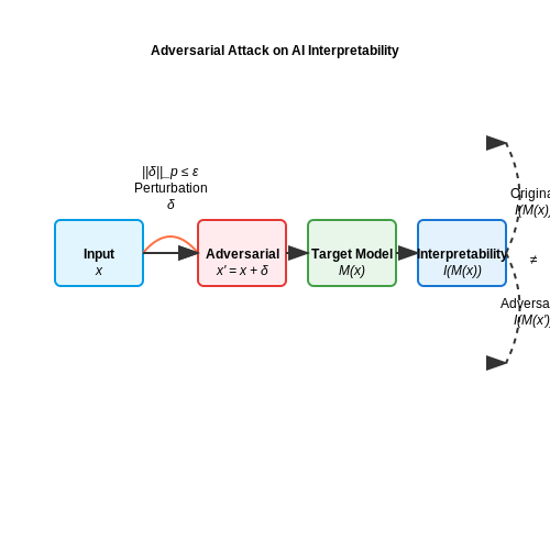
When an AI system is designed to interpret the outputs of another AI model, it inherits vulnerabilities from both the underlying model and its own architecture. Adversarial attacks exploit these vulnerabilities by introducing perturbations that are imperceptible to humans but cause misclassification or misinterpretation. Formally, given an interpretability model I and a target model M, an adversarial example x' can be crafted such that:
where x is the original input and x' = x + δ, with ||δ||_p ≤ ε for some small ε under the L_p norm.
Gradient-Based Attack Strategies
Adversarial attacks often leverage gradient information to maximize the divergence between the interpretability model's output and the true explanation. The Fast Gradient Sign Method (FGSM) can be extended to target interpretability:
where J is the loss function measuring the discrepancy between the interpretability output and the adversarial target ytarget.
Interpretation-Specific Threats
Three primary attack vectors emerge when targeting AI interpretability:
- Explanation Misalignment: The attacker forces the interpretability model to produce explanations that contradict the actual decision logic.
- Confidence Masking: The model's confidence scores are manipulated while maintaining correct predictions, misleading the interpretation.
- Feature Space Obfuscation: Perturbations are crafted to distort the feature importance rankings in methods like SHAP or LIME.
Case Study: Attacking LIME Explanations
In a 2020 study, attackers demonstrated that LIME explanations could be manipulated by strategically modifying input features. For a linear interpretability model g approximating the complex model f:
The attack successfully generated inputs where LIME attributed importance to irrelevant features while maintaining the original classification.
Defensive Strategies
Current defenses focus on three approaches:
- Interpretation Consistency Checks: Verify that explanations remain stable under small input perturbations.
- Adversarial Training: Augment training data with adversarial examples targeting interpretability.
- Certified Robustness: Provide mathematical guarantees that explanations won't change within an ε-ball around inputs.
The certified robustness approach for interpretability models can be formulated as:
where d is a distance metric between explanations and τ is a tolerance threshold.
4.3 Governance Frameworks for Responsible Deployment
Governance frameworks for AI systems that interpret other AI outputs must address both technical and ethical challenges to ensure accountability, transparency, and alignment with societal values. These frameworks typically incorporate multi-stakeholder oversight, rigorous validation protocols, and dynamic risk assessment mechanisms.
Key Components of Governance Frameworks
Effective governance relies on three core pillars:
- Technical Auditing: Continuous evaluation of model interpretability methods through quantitative metrics like faithfulness and robustness. For instance, the faithfulness score F of an interpreter model M can be computed as:
where φ(xi) represents the explanation provided by M for input xi, and 𝕀 is an indicator function checking prediction consistency under the explanation.
- Legal Compliance: Alignment with regulations like the EU AI Act, which mandates documentation of model interpretability techniques for high-risk applications.
- Ethical Review Boards: Cross-disciplinary committees that assess potential societal impacts using frameworks like ALTAI (Assessment List for Trustworthy AI).
Implementation Challenges
Deploying these frameworks encounters two principal difficulties:
- Explanation Drift: When the interpreter model's performance degrades due to distributional shifts in the base model's outputs. This can be quantified through the explanation stability index (ESI):
where φt(x) denotes explanations at time step t.
- Adversarial Exploitation: Malicious actors may craft inputs that generate misleading interpretations. Defensive measures include adversarial training of interpreter models using perturbed examples:
Case Study: Healthcare Diagnostics
In medical AI systems, the U.S. FDA's Software as a Medical Device (SaMD) framework requires:
- Validation of explanation methods against clinician judgments
- Continuous monitoring of interpretation accuracy across demographic groups
- Documentation of failure modes and mitigation strategies
A 2023 study on radiology AI systems demonstrated that governance protocols reduced diagnostic errors by 32% when interpreter models were subjected to monthly audits against ground truth annotations from multiple radiologists.
Emerging Standards
Recent initiatives are developing standardized benchmarks for AI interpretability:
| Standard | Scope | Metrics |
|---|---|---|
| IEEE P7001 | Transparency of autonomous systems | Explanation coverage, counterfactual completeness |
| ISO/IEC 23053 | ML system interpretability | Feature importance consistency, explanation fidelity |
5. Key Research Papers and Surveys
5.1 Key Research Papers and Surveys
- Explainable AI (XAI): A systematic meta-survey of current challenges ... — Explainable artificial intelligence (XAI) has been proposed as a solution that can help to move towards more transparent AI and thus avoid limiting the adoption of AI in critical domains [1], [2].Generally speaking, according to [3], XAI focuses on developing explainable techniques that empower end-users in comprehending, trusting, and efficiently managing the new age of AI systems.
- PDF Enhancing Transparency and Understanding in AI Decision-Making Processes — gap between complex AI models and human understanding, ensuring that stakeholders can trust and effectively use AI outputs. Key approaches in XAI include: • Model-Agnostic Methods: Techniques that can be applied to any AI model to provide explanations, regardless of the model's architecture.
- Explainable Artificial Intelligence: Importance, Use Domains, Stages ... — Therefore, Explainable Artificial Intelligence (XAI) has emerged to address the need for transparency in AI frameworks and to lower barriers to the widespread application of AI in important sectors. XAI is an approach to develop open techniques that let consumers comprehend and trust the evolving AI systems while being able to govern them successfully [].
- A systematic review of Explainable Artificial Intelligence models and ... — AI was developed around 1950 in the computer science sector, and it copied the human mind to develop machines that can process, methodise, and perform based on the data given to the system, which will be useful when large amounts of datasets are used [1].AI machineries widely being used in the industrial domain and prompted to do a more research works in engineering fields such as NLP (natural ...
- The promise and perils of using AI for research and writing — How and whether psychologists and students can incorporate AI tools into their research will vary depending upon the circumstances involved, said Samantha Denneny, development manager for APA Style. AI use can be unavoidable if it comprises the heart of a research project on, for instance, the role of the technology in psychology, she said.
- Chapter 5 Artificial Intelligence - Springer — 5.1.3 Understanding How does AI "understand" questions, and what does "understanding" mean for AI? Unlike humans, who use conscious thought, existing knowledge, and reasoning to reflect on the meaning, context, and implications of a question, GPT—a model of AI—relies on pattern recognition, statistical correlations, and predictive ...
- Artificial intelligence research: A review on dominant themes, methods ... — AI is still garnering attention, leading to a slow but steadily growing body of research (e.g. [5]).While these reviews have provided few valuable insights into AI in other domains [6, 7], huge knowledge gaps persist, underscoring the need for further examination of information systems (IS).Thus, AI in information systems research is a new technology for gathering information, generating ...
- (PDF) How to explain AI systems to end users: a ... - ResearchGate — users represents a key challenge for AI system design and an important area of study for XAI research. This calls for review studies provi ding evidence-based insights about end users '
- Artificial intelligence in information systems research: A systematic ... — AI has a history much longer than is commonly understood, in fields from science and philosophy ranging all the way back to ancient Greece (Dennehy, 2020), but its modern iteration owes much to Alan Turing (Turing, 1950) and conference in Dartmouth College in 1956 (McCorduck, 2004), where the term "Artificial Intelligence" was officially coined and defined by John McCarthy at the time as ...
- Requirements for Explainability and Acceptance of Artificial ... — The following paragraphs briefly introduce related technological aspects to establish a common understanding of the broader context. First, challenges and state-of-the-art of XAI are discussed from a technical perspective in Sect. 2.1.Section 2.2 then provides a human perspective on explainability in intelligent systems. Finally, Sect. 2.3 brings both perspectives together by discussing the ...
5.2 Open-Source Tools and Libraries
- Software Development Life Cycle Perspective: A Survey of Benchmarks for ... — Infibench (Li et al., 2025a) is designed for open-ended code question answering, containing 234 Stack Overflow questions, covering 15 programming languages and 5 core domains. CodeQA (Liu and Wan, 2021) focuses on source code understanding by automatically generating question-answer pairs from comments in Java and Python codebases.
- Open-source artificial intelligence - Wikipedia — Open-source artificial intelligence is an AI system that is freely available to use, study, modify, and share. [1] These attributes extend to each of the system's components, including datasets, code, and model parameters, promoting a collaborative and transparent approach to AI development. [1] Free and open-source software (FOSS) licenses, such as the Apache License, MIT License, and GNU ...
- Toward Open-Source AI Systems as Digital Public Goods ... - Springer — Open-source technologies are the backbone of our digital economy. Most websites depend on open-source servers such as Apache [], and open-source software is estimated to have a demand-side value of $8.8 trillion [].According to this research, companies' software expenses would be 3.5 times higher if open-source software were unavailable.
- Open-Source AI-based SE Tools: Opportunities and Challenges of ... — Second, despite their widespread application in many areas of software engineering, such as vulnerability detection (Li et al., 2018), they still lack the strong open-source community support typical of traditional software engineering tools.These open-source models also resemble isolated information islands, where individual entities independently complete the training and release of models ...
- AI Engineer World's Fair: Second Run, Twice The Fun — AI Reddit Recap /r/LocalLlama Recap 1. New SOTA AI Models, Benchmarks, and Training Innovations. New SOTA Apache Fine tunable Music Model! (Score: 303, Comments: 86): The ACE-Step model (Github, HuggingFace) is a newly released open-source, Apache-licensed generative model for music that is fine-tunable and features extremely fast inference: benchmarks report 3 minutes of music generated in ...
- Generative artificial intelligence - Wikipedia — Generative artificial intelligence (Generative AI, GenAI, [1] or GAI) is a subfield of artificial intelligence that uses generative models to produce text, images, videos, or other forms of data. [2] [3] [4] These models learn the underlying patterns and structures of their training data and use them to produce new data [5] [6] based on the input, which often comes in the form of natural ...
- (PDF) Characterization and Machine Learning Classification of AI and PC ... — 2020. Deep learning is a very popular machine learning method currently, and it can be used to solve various tasks. There are now many open source deep learning tools that can build various deep learning network models, such as convolutional neural network (CNN) and recurrent neural network (RNN), Generative Adversarial Networks(GANs).
- Artificial intelligence - Wikipedia — Artificial intelligence (AI) refers to the capability of computational systems to perform tasks typically associated with human intelligence, such as learning, reasoning, problem-solving, perception, and decision-making.It is a field of research in computer science that develops and studies methods and software that enable machines to perceive their environment and use learning and ...
- Broad learning systems: An overview of recent advances, applications ... — Broad learning system (BLS) as a novel training framework derived from the random vector functional link neural network (RVFLNN). Unlike RVFLNN, which…
- AD-AutoGPT: An autonomous GPT for Alzheimer's disease infodemiology — In this pioneering study, inspired by AutoGPT, the state-of-the-art open-source application based on the GPT-4 large language model, we develop a novel tool called AD-AutoGPT, which can conduct data collection, processing, and analysis about complex health narratives of Alzheimer's Disease in an autonomous manner via users' textual prompts. We collated comprehensive data from a variety of ...
5.3 Recommended Courses and Tutorials
- Google AI - Understanding AI: AI tools, training, and skills — Google offers various AI-powered programs, training, and tools to help advance your skills. Develop AI skills and view available resources.
- A Practical Tutorial on Explainable AI Techniques - arXiv.org — A query can explain AI systems by connecting different model outputs, aggregating inputs for sum-marising the behaviour of a system in specific domains or relating specific inputs with specific features against each other and the output.
- PDF mastering-generative-ai-and-prompt-engineering_FINAL — To further expand your knowledge and understanding of generative AI and prompt engineering, we have compiled a list of recommended books, articles, and courses that can provide additional insights, practical examples, and guidance.
- Introduction to Neural Networks and PyTorch | Coursera — This course is ideal for AI engineers looking to gain job-ready skills in PyTorch that will catch the eye of an employer. AI developers use PyTorch to design, train, and optimize neural networks to enable computers to perform tasks such as image recognition, natural language processing, and predictive analytics.
- Introduction to AI - Coursera — Explore the various types of AI, examine ethical considerations, and delve into the key machine learning models that power modern AI systems. Whether your goal is to work directly with AI, strengthen your software development skills, or enhance your data science expertise, this course provides an essential foundation for success in the field.
- Artificial Intelligence Courses: Online, Colleges, Eligibility ... — Artificial Intelligence Courses Online If you are interested to learn artificial intelligence, you can also pursue AI courses online. These courses provide an understanding of how computers work. They cover topics like Language Processing, Machine learning, and Robotics. Top virtual learning platforms like Coursera, Udemy, edX, and Great Learning are offering courses in artificial intelligence ...
- Professional Certificate Program in Machine Learning & Artificial ... — MIT Professional Education is pleased to offer the Professional Certificate Program in Machine Learning & Artificial Intelligence. MIT has played a leading role in the rise of AI and the new category of jobs it is creating across the world economy. Our goal is to ensure businesses and individuals have the education and training necessary to succeed in the AI-powered future. This certificate ...
- Mastering Prompt Engineering: A Guide to Effective AI Interaction — This comprehensive guide delves into the art and science of prompt engineering, offering practical techniques to formulate effective prompts that yield accurate and relevant responses from AI models.
- Online Courses - Learn Anything, On Your Schedule | Udemy — Udemy is an online learning and teaching marketplace with over 250,000 courses and 73 million students. Learn programming, marketing, data science and more.
- LinkedIn Learning: Online Training Courses & Skill Building — Accelerate skills & career development for yourself or your team | Business, AI, tech, & creative skills | Find your LinkedIn Learning plan today.