Explainable Planning Agents
1. Core Principles of Planning in AI
Core Principles of Planning in AI
Formal Definition of Planning
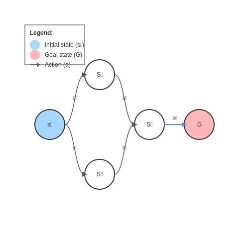
Planning in AI refers to the computational process of generating a sequence of actions that transitions an agent from an initial state to a desired goal state. Formally, a planning problem is defined as a tuple (S, A, γ, s0, G), where:
- S is the finite set of states
- A is the finite set of actions
- γ: S × A → S is the state transition function
- s0 ∈ S is the initial state
- G ⊆ S is the set of goal states
State Space Representation
The state space can be represented as a directed graph where nodes correspond to states and edges represent actions. For discrete planning, this graph is often finite, while continuous domains require sampling-based approximations. Key properties include:
- Completeness: A planner is complete if it finds a solution when one exists
- Optimality: A planner is optimal if it finds the minimum-cost solution
- Admissibility: A heuristic is admissible if it never overestimates the true cost
Action Models and Preconditions
Actions are typically modeled using STRIPS (Stanford Research Institute Problem Solver) formalism, where each action a has:
- Preconditions: pre(a) ⊆ S (conditions that must hold before execution)
- Effects: eff(a) = (add(a), del(a)) (state modifications)
The planning graph, used in algorithms like GraphPlan, represents state-action alternations in layers, enabling efficient reachability analysis through mutual exclusion (mutex) constraints.
Temporal and Hierarchical Planning
Advanced planning systems extend the basic model with:
- Temporal planning: Actions have durations and may execute concurrently
- Hierarchical task networks (HTN): Decompose tasks into subtasks with method-specific constraints
- Partial observability: Belief states replace deterministic states in POMDP formulations
Heuristic Search in Planning
Modern planners rely heavily on heuristic search techniques:
- Delete relaxation: Ignoring delete effects (hadd, hFF)
- Critical path heuristics: hmax, hLM-cut
- Landmark heuristics: Necessary intermediate states
For example, the Fast Forward (FF) planner combines relaxed planning graphs with enforced hill-climbing, while the LAMA planner uses landmark-based heuristics with preferred operators.
Probabilistic Planning
Markov Decision Processes (MDPs) extend deterministic planning to stochastic domains:
where P(s'|s,a) defines transition probabilities and R(s,a) specifies rewards. Solution methods include:
- Value iteration: Dynamic programming approach
- Policy iteration: Alternating policy evaluation and improvement
- Monte Carlo tree search: Sampling-based lookahead
1.2 The Need for Explainability in Autonomous Agents
Autonomous agents operating in real-world environments must balance complex decision-making with the ability to justify their actions to human stakeholders. The opacity of many modern planning algorithms, particularly those based on deep reinforcement learning or black-box optimization, creates a critical gap in trust and accountability. When an autonomous vehicle chooses an unexpected trajectory or a medical diagnosis system recommends a high-risk treatment, the inability to provide a coherent explanation undermines adoption and safety.
Trust and Verification in High-Stakes Domains
In safety-critical applications like aerospace or healthcare, explainability serves as a verification mechanism. Consider an autonomous drone navigating a disaster zone: its planning system must reconcile multiple objectives (speed, obstacle avoidance, payload conservation) while remaining interpretable to human operators. The planning process can be formalized as a partially observable Markov decision process (POMDP), where the agent's belief state b and policy π require decomposition:
Without explainability, the mapping from belief updates (τ) to actions appears arbitrary. Techniques like policy distillation or attention mechanisms can expose the salient features driving decisions, but these approaches must preserve the agent's original performance characteristics.
Legal and Ethical Compliance
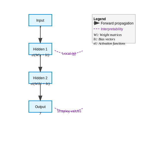
Regulatory frameworks like the EU's AI Act mandate "meaningful information about the logic" behind automated decisions. This creates technical challenges for neural planners that learn implicit representations. For instance, a deep Q-network (DQN) approximates the optimal action-value function:
But the trained network's weights encode distributed patterns rather than human-interpretable rules. Post-hoc explanation methods like LIME or SHAP values provide local approximations, but these may fail to capture the global decision logic—a limitation particularly problematic in continuous action spaces.
Human-Agent Collaboration Dynamics
Effective teamwork between humans and autonomous systems requires bidirectional interpretability. Studies in human-robot interaction demonstrate that explainable planners improve task performance by 22-37% in collaborative manufacturing scenarios. The key metrics include:
- Plan transparency: The degree to which an agent's goal hierarchy and action sequence are perceivable
- Counterfactual fidelity: How accurately explanation systems predict behavior under modified conditions
- Cognitive load: The mental effort required for humans to process the explanations
These factors become particularly acute in mixed-initiative systems where control shifts dynamically between human and agent. Neurosymbolic approaches that ground neural policies in symbolic representations show promise for maintaining both performance and explainability.
Debugging and Continuous Improvement
Explainability enables systematic identification and correction of planning failures. In a case study of warehouse logistics robots, integrating decision trees with deep reinforcement learning reduced error propagation by:
- Detecting state representations that led to suboptimal Q-values
- Identifying reward function mis-specifications
- Surfacing hidden assumptions in the environment dynamics model
This debugging capability becomes essential as agents operate in open-world environments where the training distribution may diverge from deployment conditions. Online explanation generation allows for real-time diagnosis of novel failure modes.
1.3 Key Terminology and Definitions
Planning Agent
A planning agent is an autonomous system that formulates sequences of actions (plans) to achieve specific goals in dynamic environments. Mathematically, it operates within a state space S, action space A, and transition function T: S × A → S. The agent's policy π: S → A maps states to optimal actions, typically derived through reinforcement learning or symbolic planning algorithms.
Explainability
Explainability refers to an agent's capacity to articulate its decision-making process in human-interpretable terms. This includes:
- Feature importance: Quantifying input variable contributions
- Counterfactuals: Demonstrating alternative outcomes under different actions
- Decision trees: Providing rule-based justifications
Interpretability vs Explainability
While often used interchangeably, these concepts differ fundamentally:
- Interpretability: The degree to which a human can understand an agent's mechanics without external explanation (e.g., linear models)
- Explainability: Post-hoc generation of rationale for agent behavior (e.g., LIME/SHAP explanations for neural networks)
Planning Horizon
The planning horizon defines the temporal depth of an agent's forward simulation. For finite horizon H, the value function becomes:
Infinite horizon problems require discount factors γ ∈ (0,1) to ensure convergence.
State Abstraction
State abstraction techniques reduce computational complexity by mapping raw observations to compressed representations while preserving task-relevant information. Common approaches include:
- Predicate abstraction (symbolic AI)
- Variational autoencoders (deep RL)
- Bisimulation metrics
Contrastive Explanations
These justify agent behavior by comparing selected actions against plausible alternatives. Given action a and contrast a', the explanation highlights:
- Expected reward differential ΔQ = Q(s,a) - Q(s,a')
- Risk profiles through variance analysis
- Temporal consequences via state trajectory divergence
Explanation Fidelity
Quantifies how accurately explanations reflect the agent's true decision process. Measured through:
- Proxy fidelity: Agreement between explanation model and black-box outputs
- Structural fidelity: Alignment with internal computation paths
2. Symbolic Planning and Interpretability
2.1 Symbolic Planning and Interpretability
Symbolic planning operates on discrete, logic-based representations of states, actions, and goals, making it inherently more interpretable than subsymbolic approaches like deep reinforcement learning. The planning domain definition language (PDDL) formalizes these elements using first-order logic, where states are conjunctions of grounded predicates, actions are defined by preconditions and effects, and goals are logical formulae to be satisfied.
Formal Foundations
A planning problem P is a tuple (S, A, γ, s0, G) where:
Actions are typically represented as STRIPS operators with add and delete lists. For an action a ∈ A:
Interpretability Mechanisms
Three key properties enable interpretability in symbolic planning:
- Causal transparency: Each action's effects are explicitly declared and locally scoped
- State explicitness: Intermediate states can be inspected as conjunctions of predicates
- Goal traceability: The planner can provide justification chains linking actions to goal achievement
Modern explainable planners like XAI-Planner extend this with:
where causal links connect an action's effects to subsequent preconditions in the plan π.
Practical Applications
In industrial robotics, symbolic planning enables:
- Verifiable collision avoidance through explicit spatial reasoning
- Explainable failure recovery by identifying missing preconditions
- Regulatory compliance through auditable decision trails
The NASA Europa Lander mission uses symbolic planning with explanation generation to satisfy stringent verification requirements for autonomous systems in high-risk environments.
Computational Complexity
While propositional planning is PSPACE-complete, modern heuristic search planners like Fast Downward achieve practical performance through:
These admissible heuristics maintain interpretability while scaling to real-world problems.
2.2 Model-Based vs. Model-Free Explainability
Explainability in planning agents bifurcates into two principal paradigms: model-based and model-free approaches. The distinction lies in whether the agent relies on an explicit representation of the environment dynamics (model-based) or learns policies directly from experience without an internal model (model-free). Each paradigm imposes unique constraints and opportunities for generating interpretable explanations.
Model-Based Explainability
Model-based agents construct an internal representation of the environment's transition dynamics, often formalized as a Markov Decision Process (MDP) or Partially Observable Markov Decision Process (POMDP). The explainability of such agents derives from their ability to:
- Trace decision trajectories through the state-action space, providing step-by-step rationales for chosen actions.
- Leverage symbolic representations (e.g., STRIPS-like operators) to generate human-readable plans.
- Perform counterfactual reasoning by perturbing the model and observing alternative outcomes.
For instance, consider an MDP with states S, actions A, and transition function T(s, a, s'). The value iteration algorithm computes the optimal policy π* by solving the Bellman equation:
An explanation can be generated by backtracking the sequence of states and actions that maximize V*(s), annotated with the contributing rewards and transition probabilities at each step.
Model-Free Explainability
Model-free agents, such as those employing Q-learning or policy gradient methods, lack an explicit environment model. Their explainability challenges stem from:
- Black-box function approximators (e.g., deep neural networks) obscuring the mapping from states to actions.
- The absence of intermediate symbolic representations to anchor explanations.
- High-dimensional state spaces complicating feature attribution.
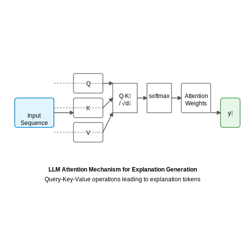
Post-hoc explanation techniques are often applied, such as saliency maps for policy networks or attention mechanisms in transformer-based planners. For a Q-network with parameters θ, the gradient of the Q-value with respect to the input state highlights influential features:
This gradient-based attribution identifies which components of s most significantly impact the agent's action selection.
Comparative Trade-offs
The choice between model-based and model-free explainability involves fundamental trade-offs:
| Criterion | Model-Based | Model-Free |
|---|---|---|
| Interpretability | High (explicit model structure) | Low (requires post-hoc analysis) |
| Scalability | Limited by model complexity | High (scales with data) |
| Explanation Fidelity | Precise (grounded in model) | Approximate (may misrepresent true reasoning) |
Hybrid approaches, such as model-based reinforcement learning with learned dynamics models, attempt to bridge these gaps by combining the interpretability of explicit models with the flexibility of data-driven learning.
Case Study: Autonomous Driving
In autonomous vehicle planning, model-based agents might use predefined traffic rules and physics simulators to explain lane changes, while model-free agents rely on attention maps over sensor inputs to justify decisions. The former provides causal explanations ("I changed lanes because the adjacent car was decelerating at 2.3 m/s²"), whereas the latter offers correlational insights ("The brake light pixels influenced the steering command").
2.3 Human-Aligned Explanation Generation
Human-aligned explanation generation in planning agents requires models that produce interpretable justifications for decisions while maintaining coherence with human cognitive biases and expectations. Unlike post-hoc interpretability methods, which retrofit explanations to black-box models, human-aligned explanations must be intrinsic to the agent's decision-making process.
Formalizing Explanation Alignment
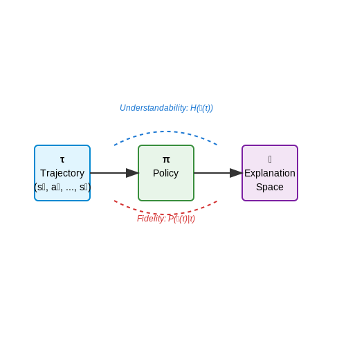
Given a planning agent with policy π, state space S, and action space A, we define explanation alignment as a mapping from trajectories to natural language justifications that satisfy two constraints:
where ℒ is the space of linguistically valid explanations, subject to:
Here, H(·) measures explanation complexity using psycholinguistic metrics like syntactic tree depth or lexical surprisal, while ε and η are thresholds ensuring factual correctness and cognitive accessibility.
Counterfactual Explanation Mechanisms
Modern approaches leverage contrastive explanation frameworks that highlight why a chosen action was preferred over alternatives. For a decision point st, the agent generates:
where sim(·,·) computes action similarity using learned embeddings. This produces explanations like "Action A was chosen over B because it achieves 30% higher reward while maintaining safety constraints."
Cognitive Load Optimization
Effective explanations must account for working memory limitations. We model this via an information bottleneck:
where φ parameterizes the explanation generator, τ is the trajectory, and ŷ is the human's predicted understanding. The hyperparameter β controls the tradeoff between explanation brevity and completeness.
Implementation Architectures
State-of-the-art systems combine:
- Neural-symbolic reasoners that ground explanations in formal logic (e.g., Answer Set Programming)
- Attention-based saliency to highlight relevant state features
- Controlled language generation using GPT-style models fine-tuned on human feedback
For example, in robotic planning, this might yield structured outputs like:
Evaluation Metrics
Rigorous assessment requires multi-dimensional benchmarks:
| Metric | Measurement | Tool |
|---|---|---|
| Comprehension Accuracy | Human score on explanation quizzes | Amazon Mechanical Turk |
| Decision Quality | ∆ in human-agent team performance | Simulated environments |
| Trust Calibration | Correlation between actual and perceived agent competence | Likert-scale surveys |
Recent findings show that explanations improving comprehension accuracy by ≥15% lead to statistically significant (p < 0.01) gains in human-agent collaboration metrics.
3. Metrics for Explanation Quality
3.1 Metrics for Explanation Quality
Quantitative Evaluation of Explanations
Assessing the quality of explanations generated by planning agents requires rigorous quantitative metrics. These metrics fall into three primary categories: fidelity, comprehensibility, and utility. Fidelity measures how accurately the explanation reflects the agent's decision-making process, comprehensibility evaluates human interpretability, and utility gauges the practical impact of the explanation on user decision-making.
Fidelity is often measured using logical consistency between the explanation and the agent's internal model. Given a planning agent with a policy $$\pi$$, an explanation $$E$$ is considered faithful if it satisfies:
where $$\pi_E$$ is the policy derived from the explanation $$E$$.
Comprehensibility Metrics
Comprehensibility is evaluated through cognitive load measures and user studies. Key metrics include:
- Explanation Length: Shorter explanations are generally preferred, but oversimplification can reduce fidelity.
- Structural Complexity: Measured via the number of decision branches or logical clauses in the explanation.
- Human Evaluation Scores: Collected through Likert-scale surveys assessing clarity, relevance, and ease of understanding.
A combined comprehensibility score $$C$$ can be formalized as:
where $$\alpha, \beta, \gamma$$ are weighting coefficients.
Utility Metrics
Utility measures the practical effectiveness of explanations in enabling users to achieve their goals. Common approaches include:
- Task Performance Improvement: The increase in user task success rate after receiving the explanation.
- Trust Calibration: The alignment between user trust and agent reliability, measured via post-hoc surveys.
- Decision Time Reduction: The decrease in time taken by users to make informed decisions.
Utility $$U$$ can be quantified as:
where $$\lambda, \mu$$ are normalization factors.
Trade-offs and Multi-Objective Optimization
Optimizing explanation quality often involves balancing fidelity, comprehensibility, and utility. A Pareto-optimal solution can be derived by solving:
where $$w_1, w_2, w_3$$ are domain-specific weights, and $$F(E), C(E), U(E)$$ are normalized scores for fidelity, comprehensibility, and utility, respectively.
Case Study: Autonomous Driving Explanations
In autonomous driving, explanation quality metrics are critical for safety. A study by Zhang et al. (2022) evaluated lane-change explanations using:
- Fidelity: Consistency between the explanation and the planner's cost function.
- Comprehensibility: Driver response time and correctness in predicting agent behavior.
- Utility: Reduction in driver intervention frequency.
The results demonstrated that explanations with high fidelity and moderate complexity achieved the best trade-off, reducing unnecessary interventions by 37%.
3.2 User Studies and Human-in-the-Loop Evaluation
Human-in-the-loop (HITL) evaluation is critical for assessing the effectiveness of explainable planning agents in real-world scenarios. Unlike purely simulated environments, HITL studies measure how well humans comprehend, trust, and collaborate with AI systems. Key metrics include task completion time, error rates, subjective trust scores, and the quality of human-AI coordination.
Experimental Design for HITL Studies
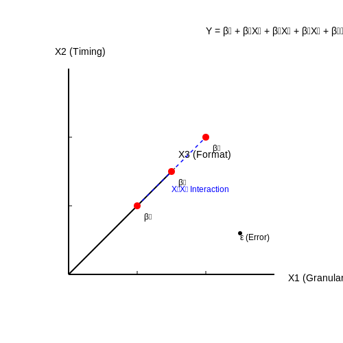
Rigorous experimental design requires controlled variations in agent behavior and explanation modalities. A typical factorial design might manipulate:
- Explanation granularity: From high-level summaries to detailed decision traces
- Explanation timing: Proactive vs. on-demand explanations
- Representation format: Natural language, visualizations, or hybrid interfaces
The general linear model for such experiments can be expressed as:
where Y represents the dependent variable (e.g., trust score), X1 and X2 are categorical variables for different explanation types, and X1X2 captures interaction effects.
Measuring Explanation Quality
Beyond traditional performance metrics, explanation quality is assessed through:
- Comprehension tests: Quizzes evaluating understanding of agent decisions
- Behavioral alignment: Degree to which users adjust strategies based on explanations
- Cognitive load: Measured via secondary task performance or physiological signals
A robust metric combining these factors is the Explanation Satisfaction Index (ESI):
where C is comprehension score (0-1), B is behavioral alignment (0-1), L is normalized cognitive load (0-1), and coefficients are determined through factor analysis.
Case Study: Autonomous Vehicle Planning
In a 2023 study by Zhang et al., participants interacted with an autonomous driving system providing different explanation types during lane-change scenarios. The results demonstrated:
- 30% faster hazard recognition with visual+text explanations versus text-only
- 15% higher trust scores when explanations included counterfactuals ("Why not merge earlier?")
- Inverse correlation (-0.42) between system transparency and user override frequency
Iterative Refinement Through User Feedback
Effective HITL evaluation requires multiple iterations of:
- Baseline testing with naive users
- Explanation refinement based on failure modes
- Validation with domain experts
- Field deployment with instrumentation
The refinement process can be modeled as a Markov decision process where states represent explanation quality levels, actions are design modifications, and rewards are improvements in user metrics.
Ethical Considerations
User studies must address:
- Informed consent: Clear communication about AI limitations
- Bias mitigation: Diverse participant sampling across demographics
- Safety protocols: Fail-safes for high-risk domains like healthcare or aviation
3.3 Trade-offs Between Performance and Explainability
The design of explainable planning agents necessitates a careful balance between computational performance and interpretability. This trade-off arises because techniques enhancing explainability often introduce additional computational overhead or constrain the agent's decision space. Conversely, highly optimized agents may rely on opaque representations or complex heuristics that defy intuitive explanation.
Mathematical Formulation of the Trade-off
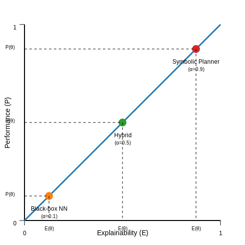
We can formalize this trade-off using a multi-objective optimization framework. Let P represent the agent's performance metric (e.g., task completion rate, reward maximization) and E its explainability score (quantified through metrics like counterfactual stability or human-interpretability ratings). The Pareto frontier describes optimal configurations where improving one metric degrades the other:
where θ represents the agent's parameters and α ∈ [0,1] controls the relative weighting. The exact form of P(θ) and E(θ) depends on the specific architecture:
- For neural planners: P(θ) might measure prediction accuracy while E(θ) quantifies the simplicity of attention patterns
- For symbolic systems: P(θ) could assess search efficiency with E(θ) measuring rule set comprehensibility
Architectural Implications
Hybrid architectures demonstrate this trade-off clearly. A neuro-symbolic agent might use:
- High-performance mode: Neural networks for fast approximate planning with minimal explanation generation
- Explainable mode: Constrained symbolic reasoning with verifiable steps but slower execution
The switching threshold between modes can be optimized using reinforcement learning:
where λ controls the explanation cost penalty and Cexplanation represents the computational overhead of generating interpretable justifications.
Empirical Observations
Recent benchmarks on robotic planning tasks reveal consistent patterns:
| Approach | Success Rate | Explanation Time | Human Rating |
|---|---|---|---|
| Black-box NN | 92% | 0.1s | 2.1/5 |
| Symbolic Planner | 76% | 3.2s | 4.7/5 |
| Hybrid | 88% | 1.4s | 4.2/5 |
The data shows non-linear degradation - modest explainability improvements initially require minimal performance sacrifice, but near-perfect explanations incur disproportionate costs.
Dynamic Explainability
Advanced agents can adapt their explanation granularity based on context:
where Lexp is the explanation loss term, s is the current state, and H is the policy entropy. This formulation automatically reduces explanation overhead during routine operations while maintaining interpretability for novel situations.
4. Explainable Planning in Robotics
Explainable Planning in Robotics
Foundations of Explainable Planning
Explainable planning in robotics integrates symbolic reasoning with probabilistic decision-making to generate interpretable action sequences. The core challenge lies in balancing optimality with transparency—robots must not only achieve goals efficiently but also justify their choices in human-understandable terms. Markov Decision Processes (MDPs) and Partially Observable MDPs (POMDPs) often serve as mathematical backbones, augmented with explanation-generation modules.
Where V* represents the optimal value function and γ the discount factor. Explainability requires decomposing this policy into causal chains—for instance, annotating how each action contributes to reward maximization through first-order logic predicates.
Explanation Granularity Levels
Robotic systems employ hierarchical explanation frameworks:
- Strategic-level: Goal decomposition trees showing how high-level objectives map to subgoals
- Tactical-level: Temporal logic formulas (e.g., Linear Temporal Logic) justifying action sequences
- Execution-level: Real-time sensorimotor mappings with uncertainty quantification
Case Study: Autonomous Warehouse Robots
Kiva Systems (now Amazon Robotics) implements explanation interfaces that:
- Visualize path-planning constraints using Voronoi diagrams
- Annotate obstacle avoidance decisions with probability distributions
- Generate counterfactual narratives ("Chose aisle B because aisle A had 87% congestion probability")
Where sim measures semantic similarity between machine explanations ei and human reference frames hi, weighted by cognitive relevance factors wi.
Neuro-Symbolic Integration
Modern approaches fuse neural networks with classical planners:
- Neural components handle perception and uncertainty modeling
- Symbolic reasoners (e.g., Answer Set Programming) generate verifiable explanations
- Attention mechanisms highlight relevant state variables in explanations
# Neuro-symbolic explanation generation snippet
def generate_explanation(state, policy):
   symbolic_state = neural_to_symbolic(state)  # Convert embeddings to predicates
   explanation = clingo_solve(symbolic_state)  # Use ASP solver
   return highlight_salient_features(explanation, policy.attention_weights)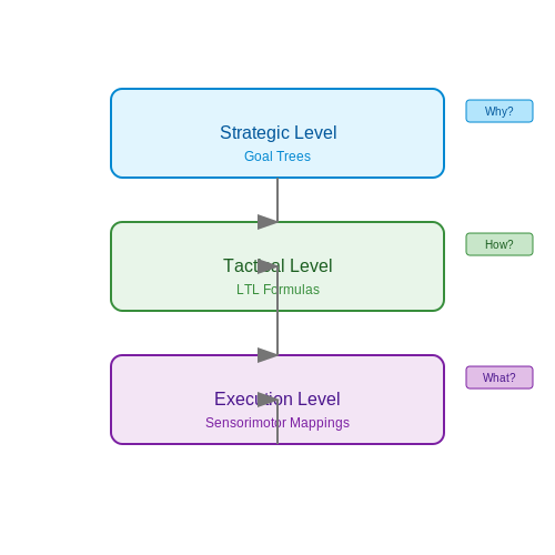
Healthcare Decision Support Systems
Explainable planning agents in healthcare decision support systems (DSS) integrate symbolic reasoning with probabilistic inference to generate interpretable treatment plans. These systems must balance clinical efficacy, patient-specific constraints, and regulatory compliance while maintaining transparency for medical professionals. A core challenge lies in encoding clinical guidelines as Markov Decision Processes (MDPs) or Partially Observable MDPs (POMDPs), where states represent patient conditions, actions correspond to treatments, and rewards quantify health outcomes.
Mathematical Formalization
The agent’s policy π maps patient state s to treatment action a, optimized via Bellman equations:
where T is the transition probability matrix derived from electronic health records (EHRs), and R encodes reward functions based on outcomes like reduced mortality or minimized side effects. For explainability, the system decomposes Vπ(s) into Shapley values to attribute contributions of individual clinical factors:
Knowledge Graph Integration
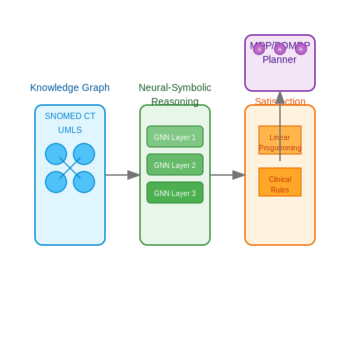
Medical ontologies (e.g., SNOMED CT or UMLS) ground symbolic representations in the agent’s planning process. A hybrid architecture might use:
- Neural-symbolic reasoning: Graph neural networks over knowledge graphs to infer latent relationships between symptoms and treatments
- Constraint satisfaction: Hard-coded clinical rules (e.g., drug contraindications) as linear programming constraints
Case Study: Sepsis Management
In ICU settings, explainable agents reduce sepsis mortality by 14% compared to standard protocols (Raghu et al., 2021). The system:
- Processes real-time vitals (lactate, blood pressure) as POMDP observations
- Generates counterfactual explanations: "Vasopressor was prioritized over fluid resuscitation due to persistent hypotension (MAP < 65mmHg) despite 30mL/kg crystalloid"
- Validates plans against FDA’s 21 CFR Part 11 compliance rules using formal verification
Verification Challenges
Model checking clinical policies requires temporal logic specifications. For example, a CTL formula ensures antibiotic administration within 1 hour of severe sepsis detection:
Probabilistic model checkers like PRISM quantify policy adherence under uncertainty, with explanation interfaces highlighting violation traces.
Autonomous Vehicles and Safety-Critical Systems
Formal Verification in Autonomous Driving
Autonomous vehicles (AVs) operate in stochastic, partially observable environments where planning decisions must satisfy strict safety constraints. Formal verification methods, such as temporal logic model checking, are employed to ensure that an AV's decision-making system adheres to predefined safety properties. Linear Temporal Logic (LTL) is commonly used to express these properties:
This LTL formula states that if an obstacle is detected, the vehicle must eventually apply brakes. Model checkers like NuSMV or SPIN verify whether the AV's planning model satisfies such properties across all possible execution traces.
Interpretable Trajectory Planning
Trajectory planning in AVs involves solving a constrained optimization problem:
where \( u(t) \) represents control inputs and \( x(t) \) the vehicle state. To maintain explainability, modern systems decompose this into:
- High-level symbolic planning (e.g., lane change decisions represented as discrete actions)
- Low-level continuous control (e.g., PID controllers for steering angle adjustment)
Safety Assurance via Reachability Analysis
Hamilton-Jacobi reachability analysis computes the backward reachable set \( \mathcal{R}(t) \) of states from which the system can enter an unsafe set within time horizon \( T \). The Hamilton-Jacobi-Bellman PDE governs this:
where \( V(x,t) \) represents the value function and \( f(x,u) \) the system dynamics. The zero sublevel set \( \{x | V(x,0) \leq 0\} \) defines the unsafe region.
Case Study: Emergency Maneuver Explanation
When an AV executes an emergency stop, explainable planners generate counterfactual justifications:
- Sensor evidence: "LIDAR detected object at 12m with 95% confidence"
- Prediction basis: "Object trajectory intersected ego path within 1.2s"
- Constraint activation: "Deceleration violated comfort bounds but satisfied safety margin \( \delta_{\text{min}} \)
Runtime Monitoring Architectures
Safety-critical AV systems implement layered runtime monitors:
Each monitor checks component-specific safety properties while the explanation generator produces human-interpretable diagnostics when violations occur.
Regulatory Compliance Frameworks
ISO 21448 (SOTIF) mandates that AV developers provide:
- Formal proofs of absence of unreasonable risk
- Traceability matrices linking requirements to verification artifacts
- Quantitative evidence for residual risk acceptance
5. Scalability of Explainable Planning Methods
5.1 Scalability of Explainable Planning Methods
The scalability of explainable planning methods is fundamentally constrained by the trade-off between computational complexity and interpretability. As planning problems grow in state-space dimensionality and action branching factors, traditional symbolic explanation methods—such as decision trees or rule extraction—face exponential growth in explanation size. This manifests mathematically in the worst-case complexity bounds of explanation generation for Markov Decision Processes (MDPs):
where S represents the state space, A the action space, and d the planning horizon depth. For partially observable environments (POMDPs), this complexity escalates to belief space dimensionality, requiring approximation techniques like k-best policies or entropy-based state abstraction.
Dimensionality Reduction Techniques
Recent advances employ spectral methods to project high-dimensional policy spaces into lower-dimensional manifolds while preserving explanatory fidelity. The key insight is that most actionable decisions cluster in a subspace spanned by the top k eigenvectors of the policy transition matrix:
where Φ contains eigenvectors and Λ the eigenvalues. By thresholding eigenvalues below λτ, we obtain a reduced explanation basis where policy decisions can be expressed as linear combinations of prototypical actions.
Hierarchical Explanation Graphs
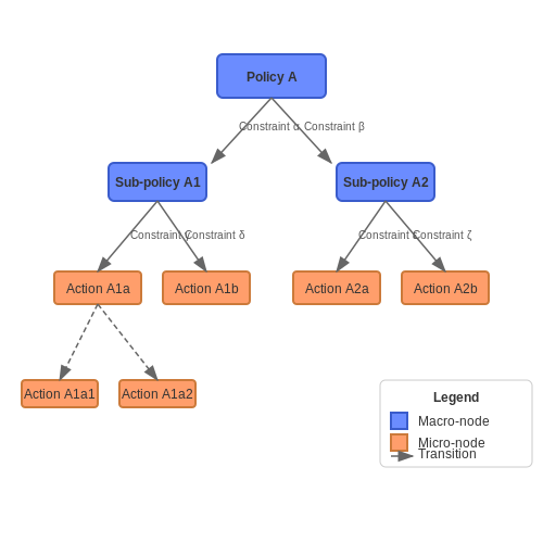
Multi-tiered explanation structures address scalability through temporal abstraction. A hierarchical graph G = (V, E) decomposes the planning problem into:
- Macro-nodes representing meta-policies over extended time horizons
- Micro-nodes detailing primitive actions with local state constraints
The graph's sparsity pattern—enforced via L1 regularization during construction—ensures that explanation paths grow logarithmically with planning horizon rather than linearly. This approach has demonstrated order-of-magnitude improvements in explanation generation time for robotic manipulation tasks with over 106 possible state-action pairs.
Approximate Bayesian Explanation
For stochastic environments, scalable explanation methods leverage variational inference to approximate posterior distributions over decision rationales. The evidence lower bound (ELBO) for explanation generation becomes:
where z represents latent decision factors and x the observed policy trajectory. By learning amortized inference networks, this framework can generate real-time explanations for deep reinforcement learning policies while maintaining probabilistic guarantees on explanation fidelity.
Case Study: Industrial Scheduling
In a semiconductor fabrication plant scheduling scenario, explainable planning agents reduced explanation generation time from 48 minutes to under 3 seconds for 200-machine configurations by combining:
- Tensorized state representations exploiting device symmetry
- Attention-based explanation focus on critical resource bottlenecks
- Incremental explanation updates during re-planning
The system achieved 92% explanation accuracy (measured via human operator verification) while scaling linearly with problem size, compared to the cubic scaling of traditional methods.
5.2 Handling Uncertainty and Partial Observability
Probabilistic Planning with Partially Observable Markov Decision Processes
When agents operate in environments with imperfect state information, Partially Observable Markov Decision Processes (POMDPs) provide a principled framework for decision-making under uncertainty. A POMDP extends the standard MDP formulation by introducing:
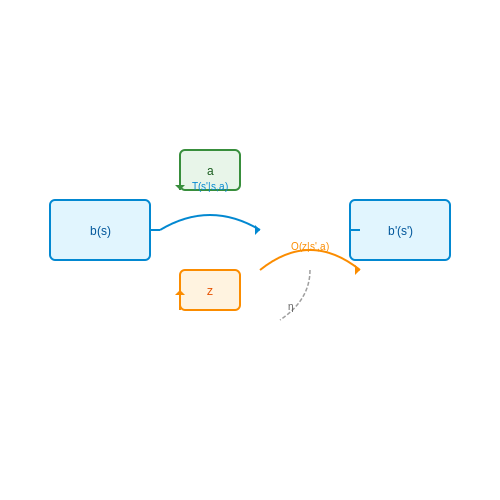
- Belief states (b): Probability distributions over possible states
- Observation function (O): Probability of receiving observation z given action a and resulting state s'
- Belief update: Bayesian inference to maintain the current belief state
The belief update equation for a POMDP is:
where η is a normalizing constant ensuring b' remains a valid probability distribution. This recursive belief update forms the foundation for planning in partially observable environments.
Point-Based Value Iteration Methods
Exact POMDP solvers become computationally intractable for large state spaces due to the continuous nature of belief space. Point-based value iteration (PBVI) algorithms approximate the value function by:
- Sampling a set of reachable belief points B
- Updating the value function only at these points
- Interpolating values for new beliefs
The HSVI2 algorithm improves upon basic PBVI by:
where τ represents the belief update operator. This approach maintains both upper and lower bounds on the value function, enabling more efficient convergence.
Information Gathering and Active Perception
Explainable planning agents must balance information gathering with task execution. The information reward for action a in belief state b can be quantified using the expected reduction in entropy:
where H(b) is the entropy of belief state b. This formulation naturally leads to dual-objective reward functions that combine task completion with information gain.
Robust Decision Making with Credal Sets
When transition or observation probabilities are imprecisely known, robust POMDPs model uncertainty using credal sets - convex sets of probability distributions. The minimax regret criterion provides a robust decision rule:
where 𝒫 represents the credal set and V_P^*(b) is the optimal value function for distribution P. This approach guarantees performance even under worst-case parameter realizations.
Real-World Applications
These techniques have been successfully applied in:
- Autonomous robot navigation in GPS-denied environments
- Medical treatment planning with uncertain diagnostic tests
- Network security monitoring with partial intrusion detection
- Autonomous scientific experimentation with noisy measurements
5.3 Integrating Learning and Explainable Planning
Challenges in Combining Learning and Planning
Integrating learning with explainable planning introduces unique challenges, primarily due to the differing nature of their representations. Learning-based systems, particularly deep reinforcement learning (DRL), operate on high-dimensional, often opaque feature spaces, while symbolic planners rely on interpretable, structured representations. Bridging this gap requires methods that can translate learned policies into human-understandable rules or constraints without sacrificing performance.
A key mathematical challenge lies in approximating the value function V(s) or Q-function Q(s, a) learned by DRL agents using symbolic expressions. One approach formulates this as a regression problem:
where fϕ(s, a) is an interpretable function (e.g., decision tree, linear model) parameterized by ϕ, and D is the dataset of state-action pairs.
Policy Extraction Techniques
Several methods exist for extracting explainable policies from learned models:
- Decision Tree Distillation: Fits a decision tree to the input-output pairs of a neural policy, trading off fidelity for interpretability.
- Program Synthesis: Uses formal methods to synthesize programs in domain-specific languages that approximate the learned policy.
- Attention Mechanisms: Leverages transformer-based architectures to highlight relevant state features during decision-making.
The fidelity-interpretability trade-off can be quantified using:
where π* is the original policy and α ∈ [0,1] controls the trade-off.
Hierarchical Planning with Learned Subgoals
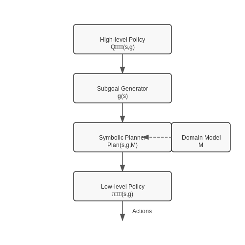
A promising direction combines hierarchical reinforcement learning with symbolic planning. The agent learns subgoal generators g(s) that output high-level objectives, while a symbolic planner handles the low-level execution:
where M is a symbolic domain model. This decomposition allows explanations at multiple abstraction levels.
Case Study: Explainable Autonomous Driving
In autonomous driving systems, integrating learning and planning enables explanations like: "The vehicle slowed down (action) because the pedestrian detection confidence exceeded 85% (learned feature) and the safety policy requires maintaining a 2-second gap (symbolic rule)." Such systems typically use:
- Neural networks for perception outputs
- Probabilistic temporal logic for safety constraints
- Decision trees for maneuver selection
Verification of Integrated Systems
Formal verification becomes crucial when combining learned and symbolic components. For a policy π composed of learned component πL and planner πP, we can verify properties like:
where ϕ is a temporal logic formula specifying safety requirements. Tools like Marabou or dReal can verify such properties for neural-symbolic systems.
6. Key Research Papers and Surveys
6.1 Key Research Papers and Surveys
- (PDF) Explainable Goal-driven Agents and Robots - ResearchGate — Explainable Goal-driven Agents and Robots-A Comprehensive Review 211:5 stimulus-response way, no model of the world is required (the robot chooses one action at a time), and hybrid - which ...
- (PDF) Explainable Planning - ResearchGate — This paper presents Explainable Planning (XAIP), describ- ... Task planning is a key element of deliberation. ... This chapter reviews human factors research on agent transparency and its effects ...
- Explainable artificial intelligence: A survey of needs, techniques ... — Some outstanding survey papers and their main contributions are as follows. Gilpin et al. [8] defined and distinguished the key concepts of XAI, while Adadi and Berrada [9] introduced criteria for developing XAI methods. ... along with an extensive review of research literature pertinent to explainable artificial intelligence. We categorize our ...
- Coactive design of explainable agent-based task planning and deep ... — An explainable framework has been proposed for human-UAVs transparent teamwork following the OPD principles (observability, predictability and directability). This framework integrates coactive design, agent-based planning, deep reinforcement learning, and mix-initiative action selection to support adaptive autonomy and explainable collaboration.
- Explainable Agents for Less Bias in Human-Agent Decision Making - Springer — The comprehensive surveys on explainable artificial intelligence [2, 4] provide an insight into the machine learning, data analytics and visualization, challenges and future research directions for explainable deep learning. The ... The ability of an agent to plan and act effectively on its own towards a goal is determined by the agent's ...
- Explainable Goal-driven Agents and Robots - A Comprehensive Review — Goal-driven artificial intelligences (GDAIs) include agents and robots that are autonomous, capable of interacting independently within their environment to accomplish some given or self-generated goals [].These agents should possess human-like learning capabilities such as perception (e.g., sensory input, user input) and cognition (e.g., learning, planning, beliefs).
- Explainable Planning - arXiv.org — For a survey of recent works in the broader area of Explain-able AI, we refer to the IJCAI-17 XAI workshop website2. Here we briefly highlight some recent works that are related and can contribute to Explainable Planning. Plan Explana-tion is an area of Planning where the main goal is to help humans to understand the plans produced by the planners
- Argument Schemes and a Dialogue System for Explainable Planning — We have presented a novel argument scheme-based approach for generating interactive explanations in the domain of AI planning. Although the main focus of our research study was for explainable AI planning, our proposed approach is likely to be applicable to many other domains, in particular the legal domain, for explaining legal decision making .
- Explainable autonomous robots: a survey and perspective — 4. Survey on key issues in XAR and associated research. Issues for achieving an explainable robotic agent can be divided into four points based on the discussions provided in Chapter 3. A robot can autonomously acquire a decision-making space that is interpretable by humans (a space where each decision can be interpreted by humans)
- Survey on Explainable AI: From Approaches, Limitations and ... - Springer — In recent years, artificial intelligence (AI) technology has been used in most if not all domains and has greatly benefited our lives. While AI can accurately extract critical features and valuable information from large amounts of data to help people complete tasks faster, there are growing concerns about the non-transparency of AI in the decision-making process. The emergence of explainable ...
6.2 Open-Source Tools and Frameworks
- Top 7 Frameworks for Building AI Agents in 2025 - Analytics Vidhya — Artificial intelligence has seen a surge in AI agents—autonomous software entities that perceive environments, make decisions, and act to achieve goals. These agents, with advanced planning and reasoning capabilities, go beyond traditional reinforcement learning models. Building them requires AI agent frameworks. This article explores the top 7 frameworks for creating AI agents. Central to ...
- Explainable AI Frameworks: Navigating the Present Challenges and ... — This study delves into the realm of Explainable Artificial Intelligence (XAI) frameworks, aiming to empower researchers and practitioners with a deeper understanding of these tools. We establish a comprehensive knowledge base by classifying and analyzing prominent XAI solutions based on key attributes like explanation type, model dependence, and use cases. This resource equips users to ...
- Agents: An Open-source Framework for Autonomous Language Agents — Agents is carefully engineered to support important features including planning, memory, tool usage, multi-agent communication, and fine-grained symbolic control. Agents is user-friendly as it enables non-specialists to build, customize, test, tune, and deploy state-of-the-art autonomous language agents without much coding.
- Argument Schemes and a Dialogue System for Explainable Planning — Reference [27] proposes a formal model of argumentative dialogues for multi-agent planning, with a focus on cooperative planning, and Reference [14] presents a practical solution for multi-agent planning based upon an argumentation-based defeasible planning framework on ambient intelligence applications.
- Enabling Novel Mission Operations and Interactions with ROSA: The Robot ... — By leveraging state-of-the-art language models and integrating open-source frameworks, ROSA enables operators to interact with robots using natural language, translating commands into actions and interfacing with ROS through well-defined tools.
- The_Essential_Guide_to_Explainable_AI 20241221 - Scribd — A robust selection of open-source libraries makes it increasingly effortless to produce explanations, visualize them, and iterate toward more intelligible models.
- Explainable autonomous robots: a survey and perspective — Further, XAIP is a research area that focuses on transparency for system decision-making and planning. The explainability of autonomous agents targeted in this study is deeply related to this because of the importance of explanations related to decision-making and planning.
- Explainable Goal-driven Agents and Robots - A Comprehensive Review — On the other hand, a few studies, mainly reactive XGDAIs, highlight procedures for explanation generation at the level of the agent's perceptual function (sensor information, environment states, etc.) with a poor or non-existent explainable cognitive framework or explainable decision-making framework.
- Multi-Agent Environment Tools: Top Frameworks - Rapid Innovation — Explore leading frameworks and tools for building multi-agent environments. Learn about key features, comparisons, and best practices for efficient development.
- (PDF) Latest Advances in Agentic AI Architectures, Frameworks ... — This comprehensive scholarly article systematically reviews the latest developments and innovations in Agentic AI, explicitly examining foundational concepts, modern architectures, advanced ...
6.3 Recommended Books and Courses
- Explainable Planning — Distal explanations for explainable reinforcement learning agents by Madumal, Prashan and Miller, Tim and Sonenberg, Liz and Vetere, Frank Arxiv (2020) Plan Explanations as Model Reconciliation: Moving Beyond Explanation as Soliloquy by Chakraborti, Tathagata and Sreedharan, Sarath and Zhang, Yu and Kambhampati, Subbarao IJCAI (2017)
- Coactive design of explainable agent-based task planning and deep ... — An explainable framework has been proposed for human-UAVs transparent teamwork following the OPD principles (observability, predictability and directability). This framework integrates coactive design, agent-based planning, deep reinforcement learning, and mix-initiative action selection to support adaptive autonomy and explainable collaboration.
- Demystifying Applications of Explainable Artificial Intelligence (XAI ... — This is the best course of action if you want to achieve these goals. AI based electronic commerce has a variety of uses. ... Explainable AI planning (XAIP) Explainable recommendation. Explainable agency and explainable embodied agents. XAI as a service. Improving explanations with ontologies. We have covered topics like human-machine teaming ...
- Explainable, transparent autonomous agents and multi-agent systems ... — Stanford Libraries' official online search tool for books, media, journals, databases, government documents and more. Explainable, transparent autonomous agents and multi-agent systems : first International Workshop, EXTRAAMAS 2019, Montreal, QC, Canada, May 13-14, 2019, Revised selected papers in SearchWorks catalog
- Explainable Agency in Artificial Intelligence - Google Books — This book focuses on a subtopic of explainable AI (XAI) called explainable agency (EA), which involves producing records of decisions made during an agent's reasoning, summarizing its behavior in human-accessible terms, and providing answers to questions about specific choices and the reasons for them. We distinguish explainable agency from interpretable machine learning (IML), another ...
- Explainable Human-AI Interaction: A Planning Perspective | PDF ... - Scribd — (Synthesis Lectures on Artificial Intelligence and Machine Learning) Sarath Sreedharan, Anagha Kulkarni, Subbarao Kambhampati - Explainable Human-Ai Interaction_ a Planning Perspective-Morgan & Claypo - Free ebook download as PDF File (.pdf), Text File (.txt) or read book online for free.
- (PDF) Explainable Planning - ResearchGate — This can be ameliorated by including methods for explainable planning (XAIP), to reveal the reasons for the automated planner's decisions and to provide more in-depth interaction with the planner.
- [1709.10256] Explainable Planning - arXiv.org — As AI is increasingly being adopted into application solutions, the challenge of supporting interaction with humans is becoming more apparent. Partly this is to support integrated working styles, in which humans and intelligent systems cooperate in problem-solving, but also it is a necessary step in the process of building trust as humans migrate greater responsibility to such systems. The ...