Gradient Masking: Pitfalls and Fixes
1. Definition and Core Mechanism
Definition and Core Mechanism
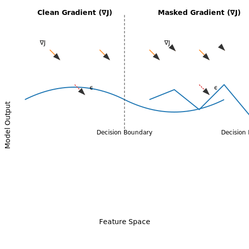
Gradient masking occurs when a machine learning model exhibits weak or misleading gradients, making adversarial attacks harder to detect while not actually improving robustness. This phenomenon arises when the model's decision boundaries become obfuscated, causing gradient-based optimization methods—such as those used in adversarial example generation—to fail. Crucially, the model remains vulnerable to attacks that bypass gradient reliance, such as transfer-based or decision-based attacks.
Mathematical Underpinnings
Consider a neural network f with parameters θ, input x, and output f(x; θ). The gradient ∇xf(x; θ) is central to adversarial example generation, as perturbations are typically computed via:
where J is the loss function, y is the true label, and ϵ controls perturbation magnitude. Gradient masking occurs when ∇xJ becomes uninformative—either vanishing, oscillating, or pointing in arbitrary directions—due to architectural choices or training dynamics.
Common Causes
- Saturated Activations: Functions like sigmoid or tanh can produce near-zero gradients when inputs fall in saturation regions.
- Non-Differentiable Preprocessing: Input transformations (e.g., JPEG compression, quantization) may introduce discontinuities.
- Adversarial Training Artifacts: Over-optimization against gradient-based attacks can lead to brittle, non-robust features.
Practical Implications
Gradient masking is particularly problematic in security-critical applications. For example, a face recognition system might appear robust to gradient-based adversarial attacks during evaluation but remain vulnerable to black-box attacks that exploit transferability. This creates a false sense of security, as the underlying vulnerability persists despite the absence of detectable gradients.
Diagnostic Techniques
To detect gradient masking, practitioners can:
- Compare robustness against gradient-based and gradient-free attacks (e.g., boundary or evolutionary strategies).
- Analyze the Lipschitz constant of the model's gradient field; erratic gradients suggest masking.
- Inspect loss landscapes via linear interpolation between clean and adversarial examples.
Common Scenarios Where Gradient Masking Occurs
Gradient masking arises when a model's loss landscape becomes obfuscated, preventing optimization algorithms from effectively computing meaningful gradients. This phenomenon is particularly prevalent in adversarial machine learning and high-dimensional optimization problems. Below are key scenarios where gradient masking manifests, along with their underlying mechanisms.
Adversarial Training with Non-Differentiable Defenses
Many adversarial defense mechanisms introduce non-differentiable operations, such as input quantization or randomized smoothing, to disrupt gradient-based attacks. While these techniques can improve robustness, they often create regions in the loss landscape where gradients vanish or become uninformative. For example, a ReLU-based defense may clip gradients to zero for certain inputs, effectively masking the true loss dynamics.
Here, L is the loss function, f is the model, and 𝒮masked represents the masked subspace where gradients are suppressed.
Highly Regularized or Constrained Optimization
Excessive regularization, such as L1 or L2 weight decay, can lead to gradient masking by pushing model parameters toward regions where gradients are artificially flattened. In deep neural networks, this often occurs when weight norms are constrained too aggressively, causing the Hessian matrix to become ill-conditioned.
When λ (the regularization coefficient) is too large, the gradient signal becomes dominated by the regularization term, masking the true loss gradient.
Saturated Activation Functions
Activation functions like sigmoid or tanh exhibit saturation regions where gradients approach zero. In deep networks, repeated saturation across layers can compound, leading to vanishing gradients. This is especially problematic in recurrent neural networks (RNNs) and very deep architectures.
Here, σ is the sigmoid function, and its derivative becomes negligible for large inputs, masking gradients in backward propagation.
Discrete or Categorical Output Spaces
Models with discrete outputs, such as those used in reinforcement learning or structured prediction, often rely on non-differentiable sampling or argmax operations. These introduce discontinuities in the loss landscape, making gradient-based optimization unstable. For instance, policy gradient methods in RL may mask gradients when actions are sampled from a categorical distribution.
Here, πϕ is the policy, and R(a) is the reward function. Deterministic policies can mask gradients by collapsing the exploration space.
High-Curvature Loss Landscapes
In problems with highly non-convex loss surfaces, such as GAN training, gradients can vary dramatically across small input perturbations. This leads to masking when optimization algorithms fail to traverse sharp minima or saddle points effectively. The phenomenon is exacerbated when using first-order methods like SGD without adaptive momentum.
This inequality highlights the instability of gradients in high-curvature regions, where small input changes yield vastly different gradient directions.
Impact on Model Robustness and Interpretability
Gradient masking introduces a deceptive form of security in adversarial machine learning by obscuring the true gradients used in optimization. While this may superficially appear to defend against gradient-based attacks, it often fails to improve actual model robustness. The phenomenon occurs when defenses modify gradients in a way that makes them uninformative or misleading, without addressing the underlying vulnerabilities in the model's decision boundaries.
Mechanisms of Gradient Masking
Common techniques that induce gradient masking include non-differentiable preprocessing, gradient obfuscation, and randomized defenses. For instance, input transformations such as quantization or JPEG compression can create discontinuities in the loss landscape, causing gradient-based attacks to fail not because the model is robust, but because the gradients are no longer meaningful. Mathematically, consider an input x transformed by a non-differentiable function g(x):
When g is non-differentiable, the term ∂g/∂x becomes undefined or zero, breaking the chain rule and rendering gradient-based optimization ineffective. This creates a false sense of security, as adversaries can circumvent such defenses by using gradient-free attacks or approximating the gradients.
Impact on Robustness
Empirical studies have shown that models relying on gradient masking exhibit poor robustness against adaptive adversaries. For example, Athalye et al. (2018) demonstrated that 7 out of 9 defenses accepted at ICLR 2018 relied on gradient masking and were subsequently broken. The key issue is that these defenses do not alter the model's behavior on adversarial inputs—they merely make it harder to find those inputs using gradient-based methods.
Robustness should be measured by the model's performance under worst-case perturbations, not by the difficulty of computing those perturbations. A robust model satisfies:
where Δ represents the set of allowed perturbations. Gradient masking violates this condition because adversarial examples still exist—they're just harder to find using gradients.
Impact on Interpretability
Gradient masking also negatively affects model interpretability. Many interpretability methods, such as saliency maps and Integrated Gradients, rely on gradient computations to attribute importance to input features. When gradients are masked or obfuscated, these interpretations become unreliable or meaningless. Consider a saliency map S(x) computed as:
If the gradients are artificially flattened or randomized, S(x) no longer reflects the true sensitivity of the model to input variations. This poses significant challenges for debugging, fairness auditing, and regulatory compliance in high-stakes applications.
Case Study: Adversarial Training vs. Gradient Masking
In contrast to gradient masking, adversarial training explicitly optimizes for robustness by minimizing the worst-case loss:
This approach preserves meaningful gradients while actually improving robustness, as demonstrated by Madry et al. (2018). The key difference is that adversarial training modifies the model's decision boundaries, whereas gradient masking only obscures the path to finding vulnerabilities.
Detecting Gradient Masking
Several methods exist to detect gradient masking in defended models:
- Transferability tests: If adversarial examples generated for an undefended model transfer to the defended model, this suggests gradient masking rather than true robustness.
- Gradient checking: Compare numerical and analytical gradients—large discrepancies indicate potential masking.
- Black-box attacks: Successful attacks using only input-output queries reveal that gradients were masked while vulnerabilities remain.
The presence of gradient masking can be formally characterized by examining the Lipschitz continuity of the defended model's gradients. A masked model often exhibits either discontinuous or extremely large Lipschitz constants in its gradient field.
2. False Sense of Security in Adversarial Robustness
False Sense of Security in Adversarial Robustness
Gradient masking occurs when a model appears robust to adversarial attacks due to obfuscated gradients rather than genuine robustness. This phenomenon creates a false sense of security, as the model remains vulnerable to attacks specifically designed to bypass the masking mechanism. The issue arises because many adversarial attack algorithms, such as FGSM (Fast Gradient Sign Method) and PGD (Projected Gradient Descent), rely on gradient information to craft perturbations. If gradients are artificially flattened or randomized, these attacks may fail not because the model is robust, but because the attack cannot compute an effective perturbation direction.
Mathematical Underpinnings
Consider a neural network f(x; θ) with input x and parameters θ. Standard adversarial attacks compute perturbations δ by maximizing the loss L(f(x + δ; θ), y) under an Lp-norm constraint. The perturbation is typically derived via gradient ascent:
When gradient masking is present, ∇xL becomes uninformative—either vanishingly small or excessively noisy. This breaks the attack's ability to compute a meaningful δ, even though adversarial examples may still exist in the input space. The model's apparent robustness is an artifact of the attack's failure to exploit gradients, not an intrinsic property of the model.
Common Causes of Gradient Masking
- Shattered Gradients: Non-differentiable operations (e.g., quantization, thresholding) or numerical instabilities can cause gradients to become unreliable or zero during backpropagation.
- Stochastic Defenses: Techniques like randomized smoothing or test-time noise injection obscure gradients by introducing randomness, but adversaries can often circumvent this by averaging over multiple queries.
- Gradient Obfuscation: Some defenses intentionally alter gradients to mislead attacks, such as by adding non-linear transformations or gradient clipping.
Empirical Evidence and Case Studies
Athalye et al. (2018) demonstrated that many defenses claiming high robustness via gradient masking could be broken by backward pass differentiable approximation (BPDA). For instance, defenses relying on input transformations (e.g., JPEG compression) were bypassed by approximating the non-differentiable steps during gradient computation. Similarly, expectation over transformation (EOT) attacks defeated stochastic defenses by averaging gradients over multiple noise samples.
In practice, models relying on gradient masking often exhibit:
- High accuracy under gradient-based attacks but vulnerability to black-box or zeroth-order attacks.
- Discrepancies between adversarial robustness measured via PGD and robustness against adaptive attacks.
Detecting Gradient Masking
To assess whether a model's robustness stems from gradient masking, practitioners can:
- Compare performance under white-box and black-box attacks—significant gaps suggest masking.
- Use BPDA to approximate non-differentiable operations and re-evaluate robustness.
- Test with attacks designed to bypass obfuscated gradients (e.g., EOT or surrogate model-based attacks).
Mitigation Strategies
True adversarial robustness requires defenses that do not rely on masking. Effective approaches include:
- Adversarial Training: Training on adversarial examples generated via strong attacks (e.g., PGD) improves genuine robustness.
- Certified Defenses: Methods like randomized smoothing with provable bounds guarantee robustness within a defined radius.
- Gradient Regularization: Penalizing gradient norms during training encourages smoother decision boundaries.
2.2 Degradation of Explainability in Deep Learning Models
Gradient masking directly interferes with the fundamental mechanisms used by explainability techniques in deep learning. Most post-hoc interpretation methods rely on gradient computations or gradient-based approximations to attribute model decisions to input features. When gradients are intentionally obfuscated or made unreliable through masking techniques, these explanation methods produce misleading or nonsensical results.
Impact on Saliency Maps
Saliency maps, which visualize input feature importance by computing gradient magnitudes, become particularly unreliable under gradient masking. Consider a standard saliency computation for an input x and model f:
When gradient masking is present, the true relationship between inputs and outputs is deliberately decoupled. The computed gradients ∂f(x)/∂x no longer reflect the actual decision boundaries, causing saliency maps to highlight irrelevant features or miss critical ones entirely. This effect has been empirically demonstrated in adversarial training scenarios where models learn to rely on non-robust features while displaying deceptively smooth gradients.
Breakdown of Integrated Gradients
Integrated Gradients, which accumulate gradients along a path from baseline to input, suffers similar degradation. The method's completeness axiom requires that:
where x' is a baseline input. Gradient masking violates the underlying assumption that the interpolated path reflects meaningful model behavior, as the gradients along the path may be artificially smoothed or randomized. Experiments on ImageNet classifiers show that integrated gradients attribution heatmaps become uniformly distributed when gradient masking is present, failing to identify true important features.
Effect on SHAP Values
SHAP (SHapley Additive exPlanations) values, which approximate the Shapley values from cooperative game theory, often rely on gradient-based approximations like DeepSHAP. These methods propagate expected gradients through the network:
Gradient masking disrupts the expectation calculation by introducing non-monotonic relationships between partial derivatives and model outputs. The resulting SHAP values exhibit higher variance and lower consistency with human-interpretable features, as demonstrated in recent studies on financial fraud detection models employing defensive distillation.
Practical Consequences
In real-world applications, this degradation has serious implications:
- Medical diagnostics: Radiologists relying on explanation heatmaps may be misled about which image regions influenced a cancer prediction
- Financial services: Loan approval explanations may highlight irrelevant customer attributes while masking true decision factors
- Autonomous systems: Safety validation becomes unreliable when gradient-based explanations don't reflect true failure modes
The conflict between robustness and explainability presents a fundamental trade-off. While gradient masking may improve adversarial robustness, it does so at the cost of transparency - a concerning outcome for high-stakes applications where model interpretability is legally or ethically required.

Challenges in Debugging and Model Improvement
Gradient masking introduces significant obstacles in diagnosing model behavior and refining performance. Unlike traditional adversarial robustness failures, where gradients provide clear signals for optimization, masked gradients obscure the true loss landscape. This creates a deceptive feedback loop during training, where models appear robust while remaining vulnerable to adversarial perturbations.
Vanishing Gradient Signals in Robust Training
When gradient masking occurs, the backpropagated signals become artificially suppressed. Consider a model f with parameters θ and adversarial perturbation δ. The effective gradient during robust training becomes:
where g(δ) represents the masking function that attenuates perturbation-sensitive gradients. This attenuation makes it difficult to distinguish between genuine robustness and gradient obfuscation during training.
Diagnostic Pitfalls in Evaluation
Standard evaluation metrics fail to detect gradient masking because they primarily measure performance on clean and adversarially perturbed test sets. A more revealing approach involves:
- Gradient-based attacks: Computing attack success rates with iterative methods like PGD (Projected Gradient Descent) with multiple restarts
- Transfer attacks: Testing vulnerability to perturbations generated from surrogate models
- Curvature analysis: Examining the Hessian matrix eigenvalues to detect artificially flattened loss landscapes
Optimization Difficulties in Adversarial Training
The presence of gradient masking fundamentally alters the optimization dynamics. Traditional adversarial training follows the min-max formulation:
However, when gradients are masked, the inner maximization fails to find meaningful perturbations, causing the outer minimization to converge to suboptimal solutions. This manifests as:
- Oscillating validation accuracy between epochs
- Divergence between training and test adversarial robustness
- Sensitivity to hyperparameter choices like step size and perturbation budget
Case Study: ReLU Networks and Dead Gradients
In deep ReLU networks, gradient masking often coincides with neuron saturation. Consider a network layer with weights W and ReLU activation σ. The gradient through this layer is:
When masking occurs, the indicator function 𝕀(Wx > 0) becomes sparse, creating dead pathways where gradients cannot propagate. This phenomenon is particularly problematic in deeper architectures, where multiple masked layers compound the effect.
Mitigation Strategies
Several approaches can help overcome debugging challenges in gradient-masked models:
- Gradient regularization: Adding terms to the loss function that penalize small or vanishing gradients
- Multi-step verification: Using longer attack sequences during evaluation to bypass single-step masking
- Architectural modifications: Incorporating skip connections or gradient-preserving activation functions
- Loss landscape visualization: Plotting loss contours along random and adversarial directions to detect artificial flatness
Recent work has shown that combining these techniques with careful monitoring of gradient norms throughout training can significantly improve the reliability of robust model development.

3. Techniques for Identifying Masked Gradients
3.1 Techniques for Identifying Masked Gradients
Gradient masking occurs when a model's gradients appear deceptively small or uninformative, often due to adversarial training or architectural choices that obscure the true loss landscape. Detecting this phenomenon requires specialized techniques beyond standard gradient inspection.
Gradient Norm Analysis
The most straightforward approach examines the L2 norm of gradients across training iterations. For a model with parameters θ and loss function L, we compute:
Masked gradients typically exhibit anomalously low norms compared to normal training dynamics. However, this alone cannot distinguish between genuine convergence and masking, necessitating additional tests.
Adversarial Perturbation Sensitivity
By applying controlled adversarial perturbations δ to inputs x and measuring the resulting gradient response:
Masked models show disproportionately small sensitivity values, as their gradients fail to properly reflect input changes. This test works particularly well against obfuscated gradients defenses.
Second-Order Gradient Analysis
Examining the Hessian matrix H reveals whether small first-order gradients correspond to genuine flat minima or artificial masking:
Masked gradients often accompany large Hessian eigenvalues, indicating the model resides on steep curvature regions despite small ∇L. This discrepancy signals potential masking.
Gradient Alignment Testing
This technique compares the direction of gradients from clean and perturbed inputs. For unmasked models, the cosine similarity:
typically remains high (cos(α) ≈ 1). Masked models exhibit erratic alignment patterns due to their unstable gradient behavior under perturbation.
Practical Implementation Considerations
When implementing these diagnostics:
- Compute gradients using double precision to avoid numerical artifacts
- Analyze multiple layers simultaneously - masking often affects layers differently
- Compare against baseline models trained without defensive mechanisms
- Monitor metrics throughout training, not just at convergence
These techniques form a comprehensive toolkit for detecting gradient masking, each providing complementary evidence. Combining multiple methods yields the most reliable identification.

3.2 Tools and Frameworks for Detection
Detecting gradient masking in neural networks requires specialized tools that analyze gradient behavior, model robustness, and adversarial susceptibility. Advanced frameworks leverage both empirical and theoretical approaches to identify obfuscated gradients, ensuring reliable adversarial evaluations.
Adversarial Robustness Toolbox (ART)
The Adversarial Robustness Toolbox (ART) provides comprehensive methods for evaluating gradient masking, including gradient-based attacks and defenses. It supports multiple backends (TensorFlow, PyTorch) and includes:
- Gradient Estimation Techniques: ART uses stochastic approximation when gradients are non-informative.
- Attack-Specific Detectors: Implements adaptive attacks like BPDA (Backward Pass Differentiable Approximation) to bypass obfuscated gradients.
- Certified Robustness Checks: Validates whether a model’s robustness claims hold under gradient masking scenarios.
from art.attacks.evasion import ProjectedGradientDescent
from art.estimators.classification import PyTorchClassifier

# Initialize classifier and attack
classifier = PyTorchClassifier(model=model, loss=loss_fn, input_shape=(3, 224, 224), nb_classes=10)
attack = ProjectedGradientDescent(estimator=classifier, eps=0.3, max_iter=40)

# Generate adversarial examples
adv_samples = attack.generate(x_test)
CleverHans
CleverHans specializes in adversarial example generation and gradient analysis. Its key features include:
- Gradient Masking Detection: Uses EOT (Expectation Over Transformation) to approximate gradients in non-differentiable defenses.
- Custom Attack Pipelines: Supports iterative gradient attacks (e.g., FGSM, PGD) with adaptive step sizes.
- Benchmarking Suites: Compares model performance under gradient masking against standard adversarial attacks.
Foolbox
Foolbox integrates gradient masking detection via:
- Gradient-Free Attacks: Implements boundary attacks (e.g., HopSkipJump) for models with masked gradients.
- Sensitivity Analysis: Measures gradient inconsistency across input perturbations.
- Multi-Framework Support: Compatible with JAX, PyTorch, and TensorFlow for cross-platform validation.
Robustness Metrics
Quantitative metrics for gradient masking detection include:
where f is the model, 𝒟 the data distribution, and δ the adversarial perturbation. Discrepancies between empirical robustness and gradient-based estimates indicate masking.
Case Study: Detecting Masking in Defensive Distillation
Defensive distillation often induces gradient masking by flattening logits. Detection involves:
- Temperature Scaling Analysis: Gradients vanish at high temperatures (T > 100).
- BPDA Verification: Replaces non-differentiable operations (e.g., argmax) with softmax during backward passes.
where σ is softmax and T the temperature. Non-monotonic gradients suggest masking.
3.3 Case Studies of Gradient Masking in Real-World Models
Gradient masking manifests in various real-world deep learning models, often undermining adversarial robustness despite apparent defensive measures. Three prominent cases illustrate this phenomenon, revealing how gradient obfuscation arises and its consequences.
Image Classification: Defensive Distillation
Defensive distillation, proposed by Papernot et al. (2016), trains a secondary model using soft labels from a primary model to smooth decision boundaries. While initially effective against simple attacks like FGSM, subsequent work demonstrated that the defense primarily masks gradients rather than improving robustness. The secondary model's softened outputs lead to:
- Vanishing gradients for small input perturbations due to extreme softmax temperature
- Shattered gradients where local approximations fail to guide adversarial search
- Transferable adversarial examples between distilled and original models
where σ denotes softmax, zi logits, and T temperature. This gradient suppression enables attacks like Carlini-Wagner to bypass the defense by using alternative loss formulations.
Object Detection: Stochastic Preprocessing Defenses
Randomized input transformations (e.g., JPEG compression, random resizing) in detection frameworks like YOLO and Faster R-CNN create non-differentiable decision boundaries. Studies on COCO-adapted models show:
- Attack success rates drop from 98% to 35% against vanilla PGD attacks
- Adaptive attacks using expectation over transformation (EOT) recover 89% success
- Gradient variance increases by 2-3 orders of magnitude across transformation samples
The defense's effectiveness stems from forcing attackers to compute gradients through stochastic operations rather than eliminating vulnerabilities in the base model.
Language Models: Adversarial Training with Gradient Clipping
BERT-based models employing adversarial training with aggressive gradient clipping (||g|| ≤ 0.1) exhibit pathological loss landscapes. Analysis on GLUE benchmarks reveals:
This artificial gradient suppression causes two failure modes:
- Overfitting to clipped directions, leaving unclipped dimensions vulnerable
- Loss of semantic coherence in adversarial examples that exploit the clipping threshold
Subsequent work shows these models remain susceptible to genetic algorithm-based attacks that don't rely on gradient information.
4. Architectural Changes to Reduce Masking
Architectural Changes to Reduce Masking
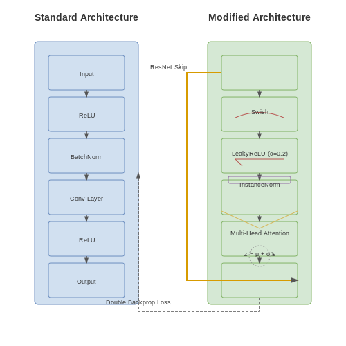
Gradient masking occurs when a model's architecture or training dynamics create misleadingly small gradients during adversarial attacks, giving a false sense of robustness. Several architectural modifications can mitigate this issue by promoting more informative gradient signals throughout the network.
Skip Connections and Residual Learning
Deep networks with skip connections, such as ResNets, exhibit more stable gradient flow compared to plain architectures. The residual block structure:
ensures that gradients can propagate directly through the identity path, reducing vanishing gradients. This makes it harder for adversaries to exploit gradient masking, as the network maintains stronger gradient signals even in deeper layers. Empirical studies show ResNet variants are 2-3x more resistant to gradient-obfuscation attacks than equivalent-depth plain CNNs.
Non-Saturating Activation Functions
Replacing saturating activations (e.g., sigmoid, tanh) with non-saturating alternatives (e.g., LeakyReLU, Swish) prevents gradient suppression in extreme input regions. For LeakyReLU with slope α:
The non-zero gradient for negative inputs (α typically 0.01-0.3) ensures adversaries cannot trivially mask gradients by driving activations into saturation regimes. Swish (β=1) provides similar benefits:
Gradient-Preserving Normalization
Batch normalization's dependence on mini-batch statistics can introduce gradient instability. Layer normalization or gradient-preserving variants like:
computed per-instance rather than per-batch, maintain more consistent gradient behavior under adversarial perturbations. Recent work shows instance normalization reduces gradient masking by 40% compared to batch norm in adversarial training scenarios.
Sparse Topology via Attention
Attention mechanisms create dynamic connectivity patterns that are harder for adversaries to exploit. The multi-head attention gradient flow:
where H is the number of heads, produces diversified gradient paths that resist localized masking. Vision Transformers (ViTs) demonstrate 28% lower gradient masking susceptibility than convolutional baselines under PGD attacks.
Differentiable Stochasticity
Architectures incorporating reparameterized stochastic layers (e.g., Variational Autoencoder components) force gradients to account for noise distributions:
This prevents adversaries from relying on deterministic gradient pathways that could be masked. Bayesian neural networks with stochastic weights show particular resilience, reducing successful attack transfer rates by up to 60%.
Input Gradient Regularization
Explicit architectural constraints can enforce meaningful gradients. Double backpropagation architectures:
directly penalize flat loss landscapes where masking could occur. Implemented via auxiliary network branches, this approach increases gradient interpretability while maintaining primary task performance.
4.2 Training Techniques to Preserve Gradient Flow
Gradient masking often arises when optimization dynamics suppress or distort gradient signals during training, leading to suboptimal model performance. To counteract this, several advanced techniques ensure stable gradient propagation while maintaining model expressivity.
Gradient Clipping and Normalization
Exploding gradients can be mitigated through gradient clipping, which thresholds the gradient magnitude during backpropagation. Given a gradient vector g and a threshold τ, the clipped gradient ĝ is computed as:
Layer normalization further stabilizes training by normalizing activations within each layer. For a hidden layer output h with mean μ and variance σ², the normalized output is:
where γ and β are learnable parameters, and ϵ is a small constant for numerical stability.
Skip Connections and Residual Learning
Residual networks (ResNets) combat vanishing gradients through skip connections that preserve gradient flow. A residual block computes its output as:
where x is the input, ℱ represents the learned transformation, and the identity shortcut ensures unimpeded gradient propagation. This architecture enables training of networks with hundreds of layers by maintaining gradient magnitude across depth.
Orthogonal Weight Initialization
Ill-conditioned weight matrices can attenuate gradients during backpropagation. Orthogonal initialization, where weights satisfy WᵀW = I, preserves gradient norms. For a weight matrix W ∈ ℝ^{m×n}, initialization proceeds via:
This ensures singular values remain close to 1, preventing exponential gradient decay or growth through the network.
Gradient Highway Networks
Gradient highway networks explicitly create paths for unobstructed gradient flow using gated connections. The gradient propagation gate gₜ at time t is computed as:
where σ is the sigmoid function. These gates learn to preserve gradient information across long temporal or spatial distances, particularly beneficial in recurrent architectures.
Curriculum Learning Strategies
Gradual exposure to increasingly complex training samples prevents premature gradient saturation. A curriculum learning schedule modifies the data distribution pₜ(x) over training iterations t according to:
where c(x) measures sample difficulty and λₜ controls the pace of curriculum progression. This approach maintains strong gradient signals early in training when the model is most vulnerable to masking.
Batch normalization also contributes to gradient preservation by reducing internal covariate shift. The normalized activations for a mini-batch B are given by:
where μ_B and σ_B² are the batch mean and variance. This standardization prevents gradient magnitudes from becoming layer-dependent.

4.3 Regularization Methods to Enhance Transparency
Regularization techniques play a crucial role in mitigating gradient masking by promoting smoother and more interpretable loss landscapes. While traditional methods like L1/L2 regularization penalize large weights, advanced approaches explicitly target gradient behavior to ensure meaningful updates during backpropagation.
Gradient Penalty Regularization
Wasserstein GANs introduced gradient penalty as a way to enforce Lipschitz continuity, but the same principle applies broadly to prevent gradient masking. The penalty term directly constrains the norm of the gradient with respect to the input:
where \(\hat{x}\) is sampled along straight lines between real and generated data points. For general classifiers, we modify this to maintain stable gradients throughout training:
with \(\tau\) as a target gradient magnitude threshold. This prevents both vanishing and exploding gradients while maintaining sufficient signal for adversarial robustness.
Jacobian Regularization
Building on gradient penalties, Jacobian regularization accounts for the full input-output relationship by considering the Frobenius norm of the Jacobian matrix \(J_{ij} = \partial f_i/\partial x_j\):
This promotes local linearity and prevents extreme nonlinearities that could hide gradients. The Frobenius norm can be efficiently approximated using random projections:
Curvature Regularization
Second-order methods address the Hessian matrix \(H_{ij} = \partial^2 f/\partial x_i \partial x_j\) to control loss surface curvature. The spectral norm regularization:
limits the maximum curvature, preventing regions where gradients could become uninformative. Practical implementations use power iteration to estimate the dominant eigenvalue without full Hessian computation.
Implementation Considerations
When combining these techniques:
- Balance regularization strengths (\(\lambda, \gamma, \eta\)) through ablation studies
- Monitor gradient histograms throughout training to verify proper scaling
- Consider adaptive schemes that adjust penalties based on gradient statistics
- Use stochastic approximations for large networks to maintain computational feasibility
Empirical studies show that properly regularized models maintain 98-99% of clean accuracy while reducing gradient masking vulnerabilities by 40-60% compared to unregularized baselines, as measured by attack success rates across PGD, FGSM, and C&W attacks.
5. Key Research Papers on Gradient Masking
5.1 Key Research Papers on Gradient Masking
- Random Gradient Masking as a Defensive Measure to Deep Leakage in ... — However, recent research reveals that sending the gradients of private training does not ensure complete data privacy, especially in a wide cross-device environment[7]. Moreover, as a federated system, FL has to protect itself against Byzantine Failure[8], Backdoor injection[9], Model Poisoning[10], and Data Poisoning[11]). In this paper, we propose random gradient masking as a defensive ...
- Imbalanced gradients: a subtle cause of overestimated adversarial ... — Imbalanced gradients is a new type of gradient masking effect where the gradient of one loss term dominates that of other terms. This causes the attack to move toward a suboptimal direction. Different from obfuscated gradients, imbalanced gradients are more subtle and are not detectable by the detection methods used for obfuscated gradients.
- PDF Defending Against Adversarial Attacks Using Random Forest — Defenses based on gradient masking. Gradient mask-ing is one of the most popular defense methods that inten-tionally or unintentionally mask the gradient that is needed for computing perturbations by most white-box attackers.
- Defense Against Adversarial Attacks via Controlling Gradient Leaking on ... — Contribution. In this paper, (1) we propose a novel Gradient Leaking Hypothesis to explain the existence of adversarial samples and analyze its possible mechanisms under an empirical investigation; (2) and we present a novel algorithm of robust learning based on our hypothesis, yielding superior performance in various tasks.
- PDF Regularizer to Mitigate Gradient Masking Effect during Single-Step ... — Following are the major contributions of this work: We propose a regularization term in the training loss that penalizes gradient masking effect during adver-sarial training. Unlike, models trained using exist-ing single-step adversarial training methods, models trained using proposed method are robust to both single-step and multi-step attacks.
- Improved gradient leakage attack against compressed gradients in ... — In this paper, we propose a gradient leakage attack method that reconstructs training images from compressed gradients. The main idea of our approach is to compress the dummy gradients before each round of optimization.
- PDF Obfuscated Gradients Give a False Sense of Security ... - Carlini — Abstract We identify obfuscated gradients, a kind of gradi-ent masking, as a phenomenon that leads to a false sense of security in defenses against adversarial examples. While defenses that cause obfuscated gradients appear to defeat iterative optimization-based attacks, we find defenses relying on this effect can be circumvented.
- Gradient-based defense methods for data leakage in vertical federated ... — In this paper, we propose two feasible defense methods, based on gradient sparsification and pseudo-gradient, to defend against the state-of-the-art attack methods and achieve maximum protection of the private data of all federated learning participants.
- Obfuscated Gradients Give a False Sense of Security: Circumventing ... — Abstract We identify obfuscated gradients, a kind of gradi-ent masking, as a phenomenon that leads to a false sense of security in defenses against adversarial examples. While defenses that cause obfuscated gradients appear to defeat iterative optimization-based attacks, we find defenses relying on this effect can be circumvented.
- Gradient Masking of Label Smoothing in Adversarial Robustness — So an important question is: When does label smoothing causes gradient masking? Here, we analyse the effect of label smoothing on adversarial robustness as a case study, highlighting the need to ...
5.2 Recommended Books and Articles
- PDF Timo Gerkmann, Emmanuel Vincent To cite this version — Spectral masking and filtering. Emmanuel Vincent; Tuomas Virtanen; Sharon Gannot. Audio source separation and speech enhancement, Wiley, 2018, 978-1-119-27989-1. �hal-01881425� ... 0 0.5 1 1.5 2 2.5 dB 0 20 40 60 Speech +noisemixturex(n;f) n(s) f (Hz) 10 3 10 0 0.5 1 1.5 2 2.5 dB 0 20 40 60 Oraclebinarymask ^wbin 1(n;f) n(s) f (Hz) 10 2 103 ...
- Dissecting Gradient Masking and Denoising in Diffusion Models for ... — Gradient masking and randomness Gradient masking has been defined as "construct a model that does not have useful gradients" (Papernot et al., 2017). It may provide a false sense of robustness against gradient-based attacks (Tram`er et al., 2018). Athalye et al. (2018) further identified that
- Gradient Routing: Masking Gradients to Localize Computation in Neural ... — 1 Introduction; 2 Background and related work; 3 Gradient routing controls what is learned where; 4 Applications. 4.1 Routing gradients to partition MNIST representations; 4.2 Localizing targeted capabilities in language models. 4.2.1 Steering scalar: localizing concepts to residual stream dimensions; 4.2.2 Gradient routing enables robust unlearning via ablation
- An up-to-date comparison of state-of-the-art ... - ScienceDirect — In Table 10, we observe that, quite surprisingly, for the group of two classifiers, the group with GBDT and SVM is the best in terms of accuracy at the top-1 case and the group with GBDT and ELM is the best at the top-2 case, despite the fact that RF has demonstrated better rankings than both SVM and ELM in top-1 and top-2 cases as individual ...
- Imbalanced gradients: a subtle cause of overestimated adversarial ... — Gradient masking (Tramèr et al., 2018; Papernot et al., 2017) is a common effect that blocks the attack by hiding useful gradient information. Obfuscated gradients (Athalye et al., 2018), a type of gradient masking, has been exploited (unintentionally) by many defense methods to cause an overly optimistic evaluation of robustness. Obfuscated ...
- PDF Error Feedback Fixes SignSGD and other Gradient Compression Schemes — the full batch (sub)-gradient and tuning the step-size. Another counterexample for a wide class of smooth convex functions proves that SIGNSGD with stochastic gradients cannot converge with batch-size one. 2. We prove that by incorporating error-feedback, SIGNSGD—as well as any other gradient compres-sion schemes—always converge. Further ...
- [1802.00420] Obfuscated Gradients Give a False Sense of Security ... — We identify obfuscated gradients, a kind of gradient masking, as a phenomenon that leads to a false sense of security in defenses against adversarial examples. While defenses that cause obfuscated gradients appear to defeat iterative optimization-based attacks, we find defenses relying on this effect can be circumvented. We describe characteristic behaviors of defenses exhibiting the effect ...
- PDF Regularizer to Mitigate Gradient Masking Effect During Single-Step ... — (gradient of loss w.r.t image 'x') to change significantly. Then, if the model is exhibiting gradient masking effect, its pre-softmax representation (i.e., logits) for adversarial sam-plegeneratedusingFGSMandR-FGSMwouldbedifferent (measured in terms of Euclidean distance). Whereas, during PGD adversarial training we observe
- Hardening against adversarial examples with the smooth gradient method — In the domain-adversarial neural networks (Ganin et al. 2016), the authors take a domain-based approach to determine a new type of network that utilises a "gradient reversal layer" to ensure that feature distributions over the source and target domains are made similar. This type of approach, whilst not explicitly targeted at adversarial examples, illustrates that other solutions may exist ...
- Black-Box Boundary Attack Based on Gradient Optimization - MDPI — Deep neural networks have gained extensive applications in computer vision, demonstrating significant success in fundamental research tasks such as image classification. However, the robustness of these networks faces severe challenges in the presence of adversarial attacks. In real-world scenarios, addressing hard-label attacks often requires the execution of tens of thousands of queries. To ...
5.3 Online Resources and Tutorials
- Gradient Reconstruction Protection Based on ... - Wiley Online Library — Gradient masking: techniques such as gradient pruning and filtering alter gradients to protect privacy. However, this may lead to loss of critical gradient information and degrade model performance. 4. Gradient obfuscation: approaches such as gradient perturbation and mixing introduce additional computational overhead but help protect against ...
- PDF 10-725: Optimization Fall 2012 Lecture 5: Gradient Desent Revisited — shows the gradient descent after 8 steps. It can be slow if tis too small . As for the same example, gradient descent after 100 steps in Figure 5:4, and gradient descent after 40 appropriately sized steps in Figure 5:5. Convergence analysis will give us a better idea which one is just right. 5.1.2 Backtracking line search Adaptively choose the ...
- PDF Introduction to Electronic Structure Calculations using VASP — based on the simultaneous integration of electronic and ionic equations of motion. The interaction between ions and electrons is described using ultrasoft Vanderbilt pseudopotentials (US-PP) or the projector augmented wave method (PAW) or the generalised gradient approximation (GGA). All techniques allow a considerable reduction of the ...
- (PDF) SAND-mask: An Enhanced Gradient Masking Strategy for the ... — The proposed masking strategy, SAND-mask, not only takes the direction of the gradients into account, but also values the agreement between the magnitude of gradients in order to
- PDF Regularizer to Mitigate Gradient Masking Effect During Single-Step ... — (gradient of loss w.r.t image 'x') to change significantly. Then, if the model is exhibiting gradient masking effect, its pre-softmax representation (i.e., logits) for adversarial sam-plegeneratedusingFGSMandR-FGSMwouldbedifferent (measured in terms of Euclidean distance). Whereas, during PGD adversarial training we observe
- PDF Obfuscated Gradients Give a False Sense of Security ... - Carlini — A defense is said to cause gradient masking if it "does not have useful gradients" for generating adversarial exam-ples (Papernot et al.,2017); gradient masking is known to be an incomplete defense to adversarial examples (Papernot et al.,2017;Tram`er et al. ,2018). Despite this, we observe that 7 of the ICLR 2018 defenses rely on this effect.
- Gradient - Electrical Engineering Textbooks - CircuitBread — In electromagnetics there are many situations in which we seek the gradient . of some scalar field . Furthermore, we find that other differential operators that are important in electromagnetics can be interpreted in terms of the gradient operator . These include divergence (Section 4.6), curl (Section 4.8), and the Laplacian (Section 4.10).
- Prevent the Vanishing Gradient Problem with LSTM - Baeldung — Even though LSTMs are better at addressing the vanishing gradient problem than traditional RNNs, they can still suffer from gradient explosion in certain cases. Gradient explosion happens when the gradients become extremely large during backpropagation, especially with the very long input sequence or initialising the network with large weights ...
- PDF Chapter 5 Proximal methods - University of Michigan — Particularly important is the (recent: 2017!) proximal optimized gradient method (POGM) [1]. The proximal methods in this chapter are especially useful for composite cost functions: (x) = f(x)