Counterfactual Explanations in AI
1. Definition and Core Concepts
Definition and Core Concepts
Counterfactual explanations provide interpretable insights into AI model decisions by answering the question: "What minimal changes to the input would lead to a different model output?" Unlike feature importance methods, which highlight influential factors, counterfactuals generate actionable, hypothetical scenarios that alter the model's prediction. This approach is rooted in causal reasoning, where counterfactuals represent perturbations in the input space that flip the model's decision boundary.
Formal Definition
Given a trained model f and an input x with prediction f(x) = y, a counterfactual explanation x' is an alternative input such that f(x') = y', where y' ≠ y. The goal is to find x' that minimizes a distance metric d(x, x') while satisfying f(x') = y'. Mathematically, this is framed as an optimization problem:
Here, d(x, x') is typically the L1 or L2 norm, ensuring minimal and interpretable changes. For instance, in a loan approval model, a counterfactual might suggest: "If your income were $5,000 higher, your application would be approved."
Key Properties of Counterfactuals
Effective counterfactual explanations must satisfy three core properties:
- Validity: The counterfactual x' must produce the desired output y' under the model f.
- Proximity: The distance d(x, x') should be small, ensuring the changes are minimal and realistic.
- Plausibility: x' must lie within the data manifold, meaning it should represent a feasible input (e.g., a valid image or realistic feature combination).
Connection to Causal Inference
Counterfactuals are deeply tied to Pearl's causal framework, where they represent interventions (do-operations) in structural causal models. Unlike purely statistical explanations, causal counterfactuals account for dependencies between features. For example, changing income might indirectly affect credit score, which must be modeled to generate realistic explanations.
This distinguishes counterfactuals from adversarial examples, which may violate causal constraints.
Practical Challenges
Generating counterfactuals involves trade-offs:
- Computational Complexity: Solving the optimization problem is NP-hard for non-linear models like neural networks.
- Discrete Features: Handling categorical variables (e.g., occupation) requires specialized distance metrics.
- Model Dependence: Counterfactuals are sensitive to model architecture; a small change in f may invalidate explanations.
Recent work addresses these via gradient-based search, genetic algorithms, or mixed-integer programming, but no universal solution exists.

Importance in Explainable AI (XAI)
Counterfactual explanations play a pivotal role in Explainable AI (XAI) by providing actionable insights into model decisions without requiring full transparency of the underlying algorithm. Unlike feature importance or saliency maps, which highlight influential inputs, counterfactuals answer the question: "What minimal changes to the input would alter the model's output?" This approach aligns with human reasoning, making it particularly valuable in high-stakes domains such as healthcare, finance, and criminal justice.
Interpretability vs. Explainability
While interpretability refers to the intrinsic simplicity of a model (e.g., linear regression), explainability involves post-hoc techniques to clarify complex models like deep neural networks. Counterfactuals bridge this gap by offering local explanations—specific to individual predictions—rather than global approximations. For instance, a loan denial explanation might state: "Your application would be approved if your income increased by $5,000." This contrasts with SHAP values or LIME, which quantify feature contributions but lack prescriptive clarity.
Mathematical Formulation
Given a model f: X → Y and an input x with prediction f(x) = y, a counterfactual explanation identifies a perturbed input x' such that:
subject to the constraint that x' is minimally distant from x under a chosen metric (e.g., L1 or L2 norm). The optimization problem is formalized as:
where d measures the distance between inputs, ℓ is a loss function penalizing incorrect predictions, and λ balances proximity and validity.
Real-World Applications
- Healthcare: Explaining why a patient was diagnosed with a high-risk condition and suggesting actionable lifestyle changes.
- Finance: Justifying credit score adjustments by specifying income or debt thresholds.
- Autonomous Systems: Debugging robotic decisions by identifying critical sensor inputs.
Advantages Over Alternative Methods
Counterfactuals avoid the reference point problem inherent in feature attribution methods (e.g., SHAP relies on baseline values). They also comply with GDPR's "right to explanation" by providing recourse rather than just transparency. However, challenges include computational cost for high-dimensional data and ensuring plausibility (e.g., suggesting biologically feasible medical interventions).
Case Study: Recidivism Prediction
In COMPAS, a controversial risk assessment tool, counterfactuals revealed that reducing prior arrests by one would flip predictions for 18% of defendants. This exposed the model's overreliance on arrest history, prompting algorithmic audits. Such analyses underscore the method's utility for bias detection and regulatory compliance.
Key Properties of Effective Counterfactuals
Effective counterfactual explanations must satisfy several key properties to ensure they are actionable, interpretable, and meaningful. These properties are derived from both theoretical considerations and empirical observations in explainable AI research.
1. Validity
A counterfactual must lead to the desired prediction when applied to the model. Formally, given a classifier f and an input x with prediction f(x), a counterfactual x' should satisfy:
Validity ensures the counterfactual is not just a hypothetical change but one that actually flips the model's decision. For probabilistic models, this can be relaxed to requiring P(y'|x') > τ for some threshold τ.
2. Proximity
The counterfactual should be as close as possible to the original input. This is typically measured using distance metrics like L1, L2, or cosine similarity. The optimization objective can be expressed as:
where d is an appropriate distance function. Proximity ensures the counterfactual is realistic and relevant to the original instance.
3. Sparsity
Effective counterfactuals should modify the fewest possible features. This aligns with the principle of minimal intervention and improves interpretability. Sparsity can be enforced using L0 regularization:
In practice, L1 regularization is often used as a convex relaxation of this NP-hard problem.
4. Actionability
Counterfactuals should only suggest changes that are feasible in the real world. This requires domain-specific constraints, such as:
- Immutable features (e.g., age, race) cannot be changed
- Some features can only increase or decrease (e.g., salary)
- Certain feature combinations must remain valid (e.g., education level and age)
5. Plausibility
The counterfactual should lie within the data manifold, meaning it should resemble realistic instances from the training distribution. This can be assessed using:
- Density estimation: pdata(x') > ε
- Machine learning: Training a discriminator to distinguish real from counterfactual instances
- Distance to nearest training instance
6. Diversity
When generating multiple counterfactuals, they should cover different possible paths to the desired outcome. Diversity can be measured as:
This property is particularly important when the counterfactual is meant to suggest multiple actionable options to a user.
7. Causal Validity
In domains where causal relationships are known, counterfactuals should respect these dependencies. For features xi that causally influence xj, changing xj without changing xi may lead to implausible examples. Causal constraints can be formalized using structural causal models.
Trade-offs and Optimization
These properties often compete with each other, requiring careful balancing. The general optimization problem for counterfactual generation can be formulated as:
where the λ parameters control the relative importance of each property. Advanced methods use gradient-based optimization, genetic algorithms, or mixed-integer programming to solve this problem.
2. Optimization-Based Approaches
Optimization-Based Approaches
Optimization-based methods formulate counterfactual explanations as a constrained optimization problem, where the goal is to find the minimal perturbation to an input that alters the model's prediction. Given a classifier f and an input x, we seek a counterfactual x' such that f(x') = y' (desired output) while minimizing a distance metric d(x, x').
Mathematical Formulation
The core optimization problem can be expressed as:
where:
- d(x, x') measures the distance between the original and counterfactual input (e.g., L1 or L2 norm),
- ℓ(f(x'), y') is a loss function penalizing deviations from the desired prediction y',
- λ balances the trade-off between proximity and prediction change.
Gradient-Based Optimization
For differentiable models (e.g., neural networks), gradient descent can efficiently solve this problem. The objective is differentiable with respect to x', allowing iterative updates:
where α is the learning rate. Constraints (e.g., feature bounds) can be enforced via projection steps.
Practical Considerations
Key challenges include:
- Feasibility: Not all x' may lie in the valid input space (e.g., pixel values in [0, 255]).
- Sparsity: L1 regularization encourages sparse perturbations (fewer feature changes).
- Diversity: Multiple counterfactuals can be found by varying initialization or adding diversity terms.
Case Study: Wachter et al.'s Approach
A seminal work frames the problem as:
This alternates between optimizing x' and updating λ to satisfy the prediction constraint. The distance metric d is often the Manhattan (L1) or Euclidean (L2) norm.
Extensions and Variants
Recent advances incorporate:
- Probabilistic guarantees: Ensuring counterfactuals are likely under the data distribution.
- Model-agnostic methods: Using black-box optimization (e.g., genetic algorithms) for non-differentiable models.
- Actionable constraints: Enforcing plausibility via domain-specific rules (e.g., "age cannot decrease").
2.2 Heuristic and Search-Based Methods
Heuristic and search-based methods generate counterfactual explanations by systematically exploring the feature space to identify minimal perturbations that alter a model's prediction. These approaches often employ optimization techniques or guided search strategies to efficiently navigate high-dimensional spaces.
Greedy Search Algorithms
Greedy algorithms iteratively modify features to minimize a cost function while ensuring the counterfactual crosses the decision boundary. At each step, the most promising feature perturbation is selected based on a local improvement criterion. The cost function typically incorporates:
- Distance metrics (e.g., L1 or L2 norm between original and counterfactual)
- Plausibility constraints (e.g., feature value ranges)
- Sparsity penalties (to minimize the number of changed features)
where d measures distance, ℓ is a loss function encouraging the desired prediction y', and λ balances these objectives.
Genetic Algorithms
Genetic algorithms evolve populations of candidate counterfactuals through selection, crossover, and mutation operations. Each candidate is evaluated using a fitness function that combines:
- Prediction validity (whether it achieves the target class)
- Proximity to the original instance
- Sparsity and plausibility metrics
The algorithm proceeds through generations, with the fittest candidates more likely to reproduce. Mutation operators introduce small perturbations, while crossover combines features from parent candidates.
Monte Carlo Tree Search (MCTS)
MCTS explores the feature space by building a search tree where nodes represent feature modifications. The algorithm balances exploration of new modifications with exploitation of promising paths through:
- Selection: Choosing nodes using Upper Confidence Bound (UCB) criteria
- Expansion: Adding new child nodes for unexplored modifications
- Simulation: Evaluating counterfactual candidates
- Backpropagation: Updating node statistics based on simulation results
where X̄i is the average reward from node i, n is the total simulations, and ni is simulations through node i.
Practical Considerations
Search-based methods must address several implementation challenges:
- Feature dependencies: Constraints must enforce realistic combinations (e.g., age cannot decrease)
- Computational cost: High-dimensional spaces require efficient search strategies
- Model queries: Black-box settings limit the number of allowed predictions
- Discrete features: Special handling for categorical and ordinal variables
Recent advances incorporate probabilistic graphical models to guide the search process by learning feature relationships from training data, improving both efficiency and plausibility of generated counterfactuals.
2.3 Model-Specific vs. Model-Agnostic Techniques
Counterfactual explanation methods bifurcate into two fundamental paradigms: model-specific and model-agnostic approaches. The distinction lies in their reliance on internal model architectures versus operating purely on input-output relationships.
Model-Specific Techniques
These methods exploit the internal structure of particular model classes. For differentiable models like neural networks, gradient-based optimization efficiently generates counterfactuals. Given a model f with parameters θ, the counterfactual search minimizes:
where y' is the desired output and λ controls proximity to the original input x. For tree-based models like random forests, techniques leverage decision paths to identify minimal feature perturbations that alter predictions.
Model-Agnostic Techniques
These approaches treat the model as a black box, requiring only query access to f(x). Optimization methods like genetic algorithms or mixed-integer programming solve:
where d is a distance metric. The Wachter method is a seminal approach that formulates this as a Lagrangian optimization problem.
Tradeoffs and Applications
Model-specific methods typically yield more efficient and precise counterfactuals but lack flexibility. For instance, a gradient-based approach for ResNets cannot be directly applied to XGBoost models. Conversely, model-agnostic techniques provide universal compatibility at the cost of computational intensity and potentially less interpretable results.
In high-stakes domains like healthcare, model-specific approaches may be preferred when transparency about the underlying reasoning is critical. For auditing heterogeneous model ensembles, model-agnostic methods become indispensable.
Mathematical Comparison
The computational complexity highlights key differences. Let n be input dimension and m be iterations:
- Model-specific: O(m·n) for gradient-based (backpropagation cost)
- Model-agnostic: O(m·n·T(f)) where T(f) is model evaluation cost
Recent hybrid approaches attempt to combine advantages, such as using surrogate differentiable models to approximate black-box behavior while retaining computational efficiency.
3. Credit Scoring and Loan Approvals
Credit Scoring and Loan Approvals
Counterfactual explanations in credit scoring provide actionable insights into why a loan application was rejected and how the applicant might alter their profile to achieve approval. Traditional black-box models, such as deep neural networks or ensemble methods, often lack transparency, making counterfactuals essential for regulatory compliance (e.g., GDPR's "right to explanation") and fairness auditing.
Mathematical Formulation
Given a classifier f and an input feature vector x, a counterfactual explanation identifies the minimal perturbation δ such that:
For credit scoring, this translates to finding the smallest changes to an applicant's attributes (e.g., income, debt-to-income ratio) that would flip the decision from "rejected" to "approved." The optimization problem is often framed as:
where ℓ is a loss function, ydesired is the target class (e.g., approval), and λ balances proximity and feasibility.
Real-World Constraints
In practice, counterfactuals must respect domain-specific constraints:
- Immutable features: Age or criminal history cannot be altered.
- Causal relationships: Increasing income might indirectly improve credit utilization.
- Actionability: Recommendations must be feasible (e.g., "increase salary by $5,000" vs. "become 10 years younger").
Case Study: FICO Score Optimization
A 2021 study demonstrated counterfactuals for FICO score improvement by perturbing five key features: credit utilization (30%), payment history (35%), credit age (15%), credit mix (10%), and new credit (10%). The generated counterfactuals prioritized reducing credit card balances over other less impactful actions, aligning with FICO's proprietary weighting.
Implementation Challenges
Generating valid counterfactuals requires addressing:
- Discrete features: Gradient-based methods fail for categorical variables (e.g., employment type). Mixed-integer programming or genetic algorithms are alternatives.
- Model dependence: Counterfactuals may not transfer between models (e.g., logistic regression vs. XGBoost).
- Multi-objective tradeoffs: Minimizing perturbation might conflict with sparsity or plausibility.
Algorithmic Approaches
Popular methods include:
- Wachter's method: Gradient descent on the counterfactual loss.
- DiCE: Diversifies counterfactuals using determinantal point processes.
- FACE: Ensures feasibility through graph-based constraints.
import dice_ml
from dice_ml.utils import helpers

dataset = helpers.load_adult_income_dataset()
d = dice_ml.Data(dataframe=dataset,
                 continuous_features=['age', 'hours_per_week'],
                 outcome_name='income')
m = dice_ml.Model(model=load_trained_model(),
                  backend='sklearn')
exp = dice_ml.Dice(d, m)
query = {'age': 22, 'hours_per_week': 45}
cf = exp.generate_counterfactuals(query,
                                 total_CFs=3,
                                 desired_class=">50K")
3.2 Healthcare Decision Support Systems
Counterfactual explanations in healthcare decision support systems provide actionable insights by answering: "What minimal changes in patient features would alter the model's prediction?" Given the high-stakes nature of medical decisions, these explanations must balance interpretability, feasibility, and clinical relevance.
Mathematical Formulation for Healthcare Counterfactuals
Let f: X → Y be a trained classifier mapping patient features x ∈ X to a clinical outcome y ∈ Y. A counterfactual x' for an instance x satisfies:
where d(·,·) is a distance metric (e.g., Manhattan or Mahalanobis distance), y' is the desired outcome, and 𝒻 represents feasible clinical constraints (e.g., biologically plausible vitals). The optimization often incorporates:
with λ terms weighting sparsity, prediction change, and feasibility penalties.
Clinical Feasibility Constraints
Unlike general ML applications, healthcare counterfactuals must respect:
- Physiological plausibility: Blood pressure cannot change from 80 mmHg to 180 mmHg instantly.
- Temporal consistency: Some features (e.g., age) are immutable; others (e.g., glucose levels) require time-sensitive interventions.
- Causal relationships: Modifying a treatment (e.g., insulin dosage) affects dependent variables (e.g., HbA1c).
These are formalized as hard constraints in the optimization problem or soft penalties via Bayesian networks encoding medical knowledge.
Case Study: Sepsis Prediction
In ICU sepsis prediction models, a counterfactual might suggest:
- Increasing systolic BP by 15 mmHg (achievable via vasopressors)
- Reducing lactate levels by 2 mmol/L (via fluid resuscitation)
- Maintaining PaO₂ > 90 mmHg (via oxygen therapy)
Such explanations directly map to clinical action pathways, unlike opaque "high-risk" scores from black-box models.
Implementation Challenges
Key technical hurdles include:
- High-dimensionality: EHR data may contain thousands of features (lab results, medications, vitals).
- Missing data: Counterfactuals must handle irregular sampling (e.g., missing lab tests) via imputation-aware methods.
- Model uncertainty: Deep learning models may exhibit prediction variance; robust counterfactuals account for confidence intervals.
Recent work addresses these via variational autoencoders for latent-space counterfactuals or adversarial training for feasibility guarantees.
Recidivism Prediction in Criminal Justice
Counterfactual explanations play a critical role in auditing recidivism prediction models, which are widely used in criminal justice systems to assess the likelihood of an individual reoffending. These models, often based on machine learning algorithms, influence decisions on parole, sentencing, and probation. However, their opacity and potential biases necessitate interpretable explanations to ensure fairness and accountability.
Mathematical Formulation of Counterfactuals in Recidivism Models
Given a trained recidivism predictor f that outputs a probability score P(y=1|x), where y=1 indicates high recidivism risk, a counterfactual explanation identifies minimal changes to input features x that would alter the prediction. Formally, for an individual with features x₀ and prediction f(x₀) = p₀, we seek:
where τ is a decision threshold (e.g., 0.5) and ||·|| is a distance metric (typically L₁ or L₂ norm). The optimization problem can be solved using gradient-based methods or heuristic search, depending on the model's differentiability.
Challenges in Criminal Justice Applications
Recidivism models often use features like prior convictions, age, and employment history, which may encode societal biases. Counterfactuals must account for immutable attributes (e.g., race) to avoid suggesting unrealistic changes. For example, a counterfactual suggesting "if the defendant were younger, the risk score would decrease" is ethically problematic and operationally useless.
Feature Sensitivity and Actionability
Actionable features (e.g., education level, substance abuse treatment) are prioritized in counterfactual generation. The following constraints are applied:
- Immutable features (e.g., race, gender) are fixed during optimization.
- Causal dependencies between features (e.g., employment → income) are enforced via constraints.
- Realistic ranges for continuous variables (e.g., age cannot decrease) are imposed.
Case Study: COMPAS Algorithm
ProPublica's analysis of the COMPAS algorithm revealed racial disparities in false-positive rates. Counterfactual explanations for COMPAS predictions highlight how non-racial features (e.g., number of juvenile arrests) disproportionately affect scores for minority defendants. For a defendant with x₀ = [prior_convictions=3, age=22, employed=No], a counterfactual might show:
This reveals that reducing prior convictions and gaining employment could lower the risk score, but the feasibility of these changes depends on systemic factors like job access.
Implementation with Gradient-Based Methods
For differentiable models (e.g., neural networks), counterfactuals are generated via gradient descent. The loss function combines prediction deviation and proximity terms:
where λ balances the two objectives. The update rule for feature j at step t is:
with learning rate η. Non-differentiable models (e.g., random forests) require genetic algorithms or mixed-integer programming.

4. Computational Complexity and Scalability
4.1 Computational Complexity and Scalability
The computational complexity of generating counterfactual explanations depends critically on three factors: the model's decision boundary complexity, the dimensionality of the input space, and the constraints imposed on the counterfactual search. For differentiable models like neural networks, gradient-based methods dominate due to their O(n) complexity relative to input dimensions, where n represents the number of features. However, for tree-based models or rule-based systems, the problem becomes NP-hard in the worst case, requiring heuristic approaches.
Formal Complexity Analysis
Consider a counterfactual search problem formulated as an optimization task:
where d measures distance between original input x and counterfactual x', and ℓ enforces the desired model output y'. The computational complexity breaks down as:
- Distance metric computation: O(n) for L1/L2 norms
- Model inference: Varies by architecture (e.g., O(n2) for attention layers)
- Constraint satisfaction: O(m) where m is the number of constraints
Dimensionality Challenges
High-dimensional spaces exhibit the curse of dimensionality for counterfactual search. The volume of valid counterfactuals decreases exponentially with dimension count, requiring more sophisticated sampling strategies. For a d-dimensional unit hypercube, the expected distance between points grows as:
This necessitates dimensionality reduction techniques or latent space optimization when dealing with complex inputs like images or text embeddings.
Scalability Techniques
Approximate Methods
Monte Carlo Tree Search (MCTS) provides polynomial-time approximations for discrete feature spaces. The upper confidence bound applied to trees (UCT) variant balances exploration and exploitation with complexity:
where b is branching factor, d is tree depth, and k is the number of iterations.
Parallelization Strategies
Modern implementations leverage GPU acceleration for batch processing of counterfactual candidates. The MapReduce paradigm enables distributed computation across feature subsets, achieving near-linear speedup for embarrassingly parallel problems.
Real-World Performance Considerations
In production systems, the 99th percentile latency often determines practical usability. For a ResNet-50 classifier generating image counterfactuals, typical timings break down as:
- Forward pass: 15ms (batch size 32)
- Gradient computation: 22ms
- Projected gradient descent steps: 50ms per iteration
This results in 200-500ms total latency for 3-5 optimization iterations, highlighting the need for model-specific optimizations.
4.2 Plausibility and Actionability of Counterfactuals
Plausibility and actionability are two critical properties that distinguish meaningful counterfactual explanations from arbitrary perturbations. A counterfactual is plausible if it represents a realistic data point within the true data distribution, while it is actionable if the suggested changes can be feasibly implemented by the user.
Plausibility Constraints
Plausibility ensures that counterfactuals are not just mathematically valid but also semantically meaningful. Formally, given a classifier f and an input x, a counterfactual x' should satisfy:
where Pdata is the data distribution and ε is a threshold for plausibility. Methods to enforce plausibility include:
- Latent space interpolation: Using autoencoders or GANs to ensure x' lies near the data manifold.
- Probabilistic modeling: Leveraging density estimators like normalizing flows to quantify Pdata(x').
- Causal constraints: Restricting changes to respect known causal relationships between features.
Actionability Constraints
Actionability requires that the modifications suggested by the counterfactual are feasible for the end user. This is often domain-specific and can be encoded as constraints:
where Iimmutable represents immutable features (e.g., age, race) and Iactionable represents modifiable features (e.g., income, education).
Optimization Framework
Combining plausibility and actionability leads to a constrained optimization problem:
where 𝒜(x) defines the set of actionable changes from x, and λ1, λ2 balance the trade-off between proximity, plausibility, and target classification.
Case Study: Loan Approval
In a loan approval system, a counterfactual suggesting "increase income by $$1 million" is implausible, while "increase income by $$5,000 and reduce debt by $2,000" may be both plausible and actionable. Domain knowledge is essential to define 𝒜(x) and plausibility thresholds.

4.3 Ethical and Fairness Considerations
Counterfactual explanations, while powerful for interpretability, introduce ethical challenges that must be rigorously addressed to prevent unintended harm. The generation of counterfactuals can inadvertently reinforce biases present in the training data or model architecture, particularly when sensitive attributes like race, gender, or socioeconomic status are involved. For instance, a counterfactual suggestion to increase income by 20% to secure a loan approval may systematically disadvantage marginalized groups if the underlying model correlates income with protected attributes.
Bias Propagation in Counterfactual Generation
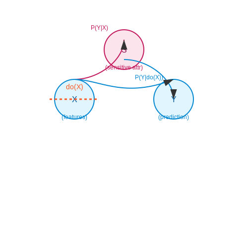
The fairness of counterfactual explanations depends on the causal structure of the model. Let X represent input features, Y the model's prediction, and S sensitive attributes. A counterfactual explanation modifies X to X' such that f(X') ≠ f(X), but if X and S are causally entangled, the explanation may inherit bias. Mathematically, this can be formalized using Pearl's do-calculus:
Here, do(X = x') denotes an intervention to set X to x', while the observational conditional probability P(Y | X = x', S = s) may capture spurious correlations. Counterfactuals that ignore this distinction risk prescribing changes that are impractical or discriminatory for certain subgroups.
Fairness Metrics for Counterfactuals
To quantify fairness, we can adapt existing metrics like demographic parity or equalized odds to the counterfactual domain. For a set of counterfactual explanations C, demographic parity requires:
where s denotes membership in a protected group. However, this alone is insufficient; the feasibility of counterfactuals must also be equitable. A proposed metric, counterfactual fairness ratio (CFR), evaluates whether the effort required to achieve a favorable outcome is consistent across groups:
where d(·,·) is a distance metric (e.g., Manhattan distance) between original and counterfactual features. A CFR deviating significantly from 1 indicates systemic bias.
Mitigation Strategies
Three principal approaches exist to align counterfactual explanations with fairness:
- Causal-aware generation: Integrate causal graphs to isolate sensitive attributes from permissible feature modifications.
- Adversarial debiasing: Train the explanation generator with a fairness loss term that penalizes disparate impact.
- Constraint-based optimization: Enforce hard constraints during counterfactual search to prevent recommendations that correlate with protected attributes.
For example, in a credit scoring model, causal-aware generation would prohibit counterfactuals that suggest changing ZIP codes (a proxy for race) while allowing adjustments to debt-to-income ratios. This requires explicit modeling of the causal relationship:
where Pa(Y) are the parents of Y in the causal graph, and λ controls the strength of the constraint.
Regulatory and Practical Implications
The EU's AI Act and Algorithmic Accountability Act in the U.S. increasingly mandate right to explanation provisions, which counterfactuals help satisfy. However, without fairness guarantees, these explanations could violate anti-discrimination laws. In healthcare, for instance, a counterfactual suggesting lower BMI to reduce predicted diabetes risk might ignore genetic factors disproportionately affecting certain ethnicities, potentially leading to clinically harmful recommendations.
5. Key Research Papers and Surveys
5.1 Key Research Papers and Surveys
- Redefining Counterfactual Explanations for Reinforcement Learning ... — Additionally, we explore the differences between counterfactual explanations in supervised learning and RL and identify the main challenges that prevent the adoption of methods from supervised in reinforcement learning. Finally, we redefine counterfactuals for RL and propose research directions for implementing counterfactuals in RL.
- PDF Designing Explainable and Counterfactual-Based AI Interfaces for ... — This work focuses on counterfactual explanations to clarify AI predictions, particularly within the paper manufacturing industry's pulping process. The main research question revolves around designing coun- terfactual explanations for multi-horizon forecasting problems using multivariate time series data in pro- cess industries.
- Categorical and Continuous Features in Counterfactual Explanations of ... — Recently, eXplainable AI (XAI) research has focused on the use of counterfactual explanations to address interpretability, algorithmic recourse, and bias in AI system decision-making. The developers of these algorithms claim they meet user requirements in generating counterfactual explanations with "plausible," "actionable" or "causally important" features. However, few of these ...
- Counterfactual Explanations and Algorithmic Recourses for Machine ... — A burgeoning body of research seeks to define the goals and methods of explainability in machine learning. In this article, we seek to review and categorize research on counterfactual explanations, a specific class of explanation that provides a link between what could have happened had input to a model been changed in a particular way.
- PDF Counterfactual Explanations for Machine Learning: A Review — A burgeoning body of research seeks to define the goals and methods of explainability in machine learning. In this paper, we seek to re-view and categorize research on counterfactual explanations, a specific class of explanation that provides a link between what could have happened had input to a model been changed in a particular way.
- A Survey of Counterfactual Explanations: Definition, Evaluation ... — In addition, we investigate the application of counterfactual explanations in two areas: model robustness, and generating feature importance. The findings demonstrate that the qualities necessary for counterfactual instances cannot be simultaneously satisfied by present methodologies. Finally, we go over potential future research directions.
- PDF A Survey of Counterfactual Explanations: Definition, Evaluation ... — In addition, we investigate the application of counterfactual explanations in two areas: model robustness, and gener-ating feature importance. The findings demonstrate that the qualities necessary for counterfactual instances cannot be simultaneously satisfied by present methodologies. Finally, we go over potential future research directions.
- Benchmarking Instance-Centric Counterfactual Algorithms for XAI: From ... — Recently, counterfactual explanations are considered an important post-hoc method that gives persuasive explanations for users to understand the internal mechanisms of AI models [9, 14, 30, 59, 93]. Unlike scoring or feature attribution explanation methods, which express each feature's (relative) relevance to the model's output [62], counterfactual explanations show which modifications ...
- PDF Counterfactual Explanations May Not Be the Best Algorithmic Recourse ... — Though there has been extensive human-AI inter- action research on explanations, translating these fndings to the algorithmic recourse setting is non-obvious due to meaningful problem setting diferences, leaving the question of whether coun- terfactuals are the most optimal explanation paradigm for recourse unanswered.
- PDF Even If Explanations: Prior Work, Desiderata & Benchmarks for Semi ... — In this paper, we survey a less-researched special-case of the counterfactual, semi-factual explanations. In this review, we survey the literature on semi-factuals, we define desiderata for this strategy, identify key evaluation metrics and imple-ment baselines to provide a solid base for future work.
5.2 Open-Source Tools and Libraries
- Categorical and Continuous Features in Counterfactual Explanations of ... — The burgeoning prevalence of automated decision-making in the public and private sectors has led to increased concerns about the fairness, transparency, and trustworthiness of these artificial intelligence (AI) systems [3, 14].Automated counterfactual explanations have emerged as a common strategy to help users understand the decisions of such systems and address fairness and trust issues [35 ...
- Introducing User Feedback-Based Counterfactual Explanations (UFCE ... — Machine learning models are widely used in real-world applications. However, their complexity makes it often challenging to interpret the rationale behind their decisions. Counterfactual explanations (CEs) have emerged as a viable solution for generating comprehensible explanations in eXplainable Artificial Intelligence (XAI). CE provides actionable information to users on how to achieve the ...
- Counterfactual explanations as interventions in latent space — Explainable Artificial Intelligence (XAI) is a set of techniques that allows the understanding of both technical and non-technical aspects of Artificial Intelligence (AI) systems. XAI is crucial to help satisfying the increasingly important demand of trustworthy Artificial Intelligence, characterized by fundamental aspects such as respect of human autonomy, prevention of harm, transparency ...
- SeldonIO/alibi: Algorithms for explaining machine learning models - GitHub — The explanation returned is an Explanation object with attributes meta and data.meta is a dictionary containing the explainer metadata and any hyperparameters and data is a dictionary containing everything related to the computed explanation. For example, for the Anchor algorithm the explanation can be accessed via explanation.data['anchor'] (or explanation.anchor).
- Redefining Counterfactual Explanations for Reinforcement Learning ... — Although explanations targeted at non-experts are necessary for user trust and human-AI collaboration, the majority of explanation methods for AI are focused on developers and expert users. Counterfactual explanations are local explanations that offer users advice on what can be changed in the input for the output of the black-box model to change.
- Explainable AI (XAI) Using LIME - GeeksforGeeks — Output: Intercept 20.03666971464815 Prediction_local [33.88485397] Right: 34.323999999999984 XAI LIME explanations. Interpreting the output: From the visualizations, we can conclude that the relatively higher price value (depicted by a bar on the left) of the house depicted by the given vector can be attributed to the following socio-economic reasons:
- GANterfactual—Counterfactual Explanations for Medical Non-experts Using ... — Contrary, counterfactual explanation systems try to enable a counterfactual reasoning by modifying the input image in a way such that the classifier would have made a different prediction. By doing so, the users of counterfactual explanation systems are equipped with a completely different kind of explanatory information.
- The Intriguing Relation Between Counterfactual Explanations and ... — The same method that creates adversarial examples (AEs) to fool image-classifiers can be used to generate counterfactual explanations (CEs) that explain algorithmic decisions. This observation has led researchers to consider CEs as AEs by another name. We argue that the relationship to the true label and the tolerance with respect to proximity are two properties that formally distinguish CEs ...
- On generating trustworthy counterfactual explanations — Visualization of the counterfactual explanations In the depicted Pareto front approximations for every experiment (in the form of three-dimensional scatter plots, parallel lines visualizations and chord diagrams), several specific counterfactual examples scattered over the front are highlighted with coloured markers. These markers refer to the ...
- Alterfactual Explanations -- The Relevance of Irrelevance for ... — A sample document descriptor with explanations. In the Combination condition, both an alter-and a counterfactual explanation were shown. Subjects in the Alterfactual and Counterfactual conditions ...
5.3 Recommended Books and Courses
- Info-CELS: Informative Saliency Map-Guided Counterfactual Explanation ... — As the demand for interpretable machine learning approaches continues to grow, there is an increasing necessity for human involvement in providing informative explanations for model decisions. This is necessary for building trust and transparency in AI-based systems, leading to the emergence of the Explainable Artificial Intelligence (XAI) field. Recently, a novel counterfactual explanation ...
- Categorical and Continuous Features in Counterfactual Explanations of ... — The burgeoning prevalence of automated decision-making in the public and private sectors has led to increased concerns about the fairness, transparency, and trustworthiness of these artificial intelligence (AI) systems [3, 14].Automated counterfactual explanations have emerged as a common strategy to help users understand the decisions of such systems and address fairness and trust issues [35 ...
- Explainable AI with counterfactual paths - arXiv.org — Explainable AI (XAI) has emerged as a promising solution to this problem by providing human-understandable explanations of AI decision-making. One approach to XAI is through the use of counterfactual explanations, which in-volve generating alternative scenarios that could have led to different outcomes. arXiv:2307.07764v1 [cs.AI] 15 Jul 2023
- CX-ToM: Counterfactual explanations with theory-of-mind for enhancing ... — We propose CX-ToM, short for counterfactual explanations with theory-of-mind, a new explainable AI (XAI) framework for explaining decisions made by a deep convolutional neural network (CNN).In contrast to the current methods in XAI that generate explanations as a single shot response, we pose explanation as an iterative communication process, i.e., dialogue between the machine and human user.
- Adapting to Change: Robust Counterfactual Explanations in ... - Springer — To the best of our knowledge, this is the first work on Graph Counterfactual Explainability (GCE) considering distributional drift happening in time. While updating (or even retraining) the prediction model under distributional drifts has been extensively explored [ 3 , 9 , 15 , 26 ], aligning counterfactual explanations after a drift happens ...
- Good Counterfactuals and Where to Find Them: A Case-Based ... - Springer — In recent years, there has been a tsunami of papers on Explainable AI (XAI) reflecting concerns that recent advances in machine learning may be limited by a lack of transparency (see e.g., [1, 2]) or by government regulation (e.g., GDPR in the EU, see [3, 4]; for reviews [5,6,7]).Historically, Case-Based Reasoning (CBR) has always given a central role to explanation, as predictions can readily ...
- Redefining Counterfactual Explanations for Reinforcement Learning ... — Although explanations targeted at non-experts are necessary for user trust and human-AI collaboration, the majority of explanation methods for AI are focused on developers and expert users. Counterfactual explanations are local explanations that offer users advice on what can be changed in the input for the output of the black-box model to change.
- On the robustness of sparse counterfactual explanations to adverse ... — The field of eXplainable AI (XAI) studies methods to dissect and analyze black-box models [8], [9] (as well as methods to generate interpretable models when possible [10]).Famous methods of XAI include feature relevance attribution [11], [12], explanation by analogy with prototypes [13], [14], and, of focus in this work, counterfactual explanations.
- On generating trustworthy counterfactual explanations — Visualization of the counterfactual explanations In the depicted Pareto front approximations for every experiment (in the form of three-dimensional scatter plots, parallel lines visualizations and chord diagrams), several specific counterfactual examples scattered over the front are highlighted with coloured markers. These markers refer to the ...
- A Survey of Counterfactual Explanations: Definition, Evaluation ... — 2.1 Contrast Explanation. According to a study in cognitive science, people don't always want to know every reason that could have caused an event, which is usually irrational and unimportant [].A comparison, or an explanation of why this event occurred as opposed to one that people would prefer to occur, provides a more insightful justification for the explanation.