Post-Hoc Explainability Pipelines for Diffusion Models
1. Core Principles of Diffusion Processes
Core Principles of Diffusion Processes
Diffusion models operate by gradually perturbing data with Gaussian noise and then learning to reverse this process. The forward diffusion process is defined as a Markov chain that systematically adds noise to the data over T timesteps. Given an initial data point x0 sampled from the true data distribution q(x), the forward process generates a sequence x1, x2, ..., xT by applying a noise schedule βt at each step.
Forward Diffusion Process
The forward process is mathematically described by the following transition kernel:
where βt is a noise schedule such that 0 < βt < 1. The cumulative effect of this process over T steps can be expressed in closed form:
where αt = 1 - βt and \(\bar{\alpha}_t = \prod_{s=1}^t \alpha_s\). This formulation allows sampling xt directly from x0 without iterating through all intermediate steps.
Reverse Diffusion Process
The reverse process learns to denoise the data by approximating the posterior q(xt-1 | xt, x0). Under Gaussian assumptions, this posterior is tractable and given by:
where the mean \(\tilde{\mu}_t\) and variance \(\tilde{\beta}_t\) are derived as:
The model learns to predict either the noise component or the original data x0 at each timestep, enabling iterative denoising.
Training Objective
Diffusion models optimize a variational lower bound on the data likelihood. The loss function simplifies to predicting the noise ε added at each step:
where εθ is a neural network trained to estimate the noise. This objective is computationally efficient and avoids the need for adversarial training.
Practical Considerations
In practice, the noise schedule βt is critical for model performance. Common choices include linear, cosine, or learned schedules. The number of timesteps T typically ranges from hundreds to thousands, with more steps yielding higher sample quality at the cost of slower generation.
Recent advancements, such as denoising diffusion implicit models (DDIM), introduce non-Markovian forward processes to accelerate sampling while maintaining sample quality. These methods enable deterministic sampling trajectories, reducing the required number of steps by an order of magnitude.
Forward and Reverse Diffusion Mechanisms
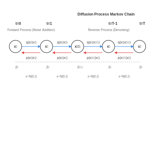
Diffusion models operate through two fundamental processes: the forward diffusion process, which gradually corrupts data by adding noise, and the reverse diffusion process, which learns to denoise and reconstruct the original data. These mechanisms are mathematically grounded in stochastic differential equations (SDEs) and their discretized counterparts.
Forward Diffusion Process
The forward process is defined as a Markov chain that incrementally adds Gaussian noise to the data over T timesteps. Given an initial data point x0 sampled from the true data distribution q(x), the noised version at step t is:
where βt is the noise schedule controlling the rate of corruption. The cumulative effect over T steps can be derived in closed form:
with αt = 1 - βt and ᾱt = ∏ts=1 αs. This formulation enables efficient sampling of any intermediate noisy state xt directly from x0.
Reverse Diffusion Process
The reverse process learns to invert the diffusion by estimating the noise component at each step. The key insight is that for small βt, the reverse transition q(xt-1 | xt) is also Gaussian. A neural network εθ is trained to predict the noise:
The mean μθ is typically parameterized as:
Training minimizes the variational lower bound on the negative log-likelihood, which simplifies to a noise prediction objective:
Practical Considerations
In practice, the noise schedule βt follows either a linear or cosine-based progression to balance training stability and sample quality. The reverse process is often accelerated using techniques like:
- DDIM (Denoising Diffusion Implicit Models): Non-Markovian sampling that skips intermediate steps while maintaining sample quality.
- Stochastic Samplers: Introduce controlled randomness during generation to improve diversity.
The interplay between forward and reverse processes enables diffusion models to generate high-fidelity samples while maintaining tractable likelihoods, making them particularly suitable for explainability analyses through perturbation-based attribution methods.

Training Objectives and Loss Functions
Diffusion models learn to reverse a fixed forward noising process by minimizing a loss function that measures the discrepancy between predicted and actual noise. The most common training objective is derived from variational lower bounds on the log-likelihood, but practical implementations often use simplified variants that trade off computational tractability against theoretical purity.
Denoising Score Matching
The fundamental loss function for diffusion models stems from denoising score matching, where the model εθ learns to predict the noise component added during the forward process. For a given timestep t and noise schedule βt, the objective becomes:
where αt = 1 - βt and ᾱt = Πts=1αs. This formulation connects to stochastic differential equations through the approximation of score functions, with the model effectively learning to estimate the gradient of the perturbed data distribution.
Hybrid Loss Formulations
Advanced diffusion architectures often employ hybrid objectives that combine multiple loss terms:
- Perceptual losses using pre-trained VGG or CLIP embeddings to maintain semantic consistency
- Adversarial components from GAN frameworks to sharpen output quality
- KL-divergence terms for explicit likelihood optimization
The general form of such hybrid losses can be expressed as:
where the λ coefficients control the relative weighting of each objective. Recent work has shown that adaptive weighting schemes based on signal-to-noise ratios can significantly improve training stability.
Explainability-Specific Objectives
When designing post-hoc explanation pipelines, additional loss terms are introduced to ensure interpretability:
where R(z) represents a regularization term acting on latent variables z to encourage disentangled or human-interpretable representations. Common choices include:
- Total correlation penalties for independence between latent dimensions
- Sparsity-inducing L1 norms on attention weights
- Maximum mean discrepancy (MMD) terms to align latent distributions with known priors
These modifications must be carefully balanced to maintain the primary generation quality while enabling effective post-hoc analysis. The temperature parameter γ typically follows an annealing schedule during training.
Gradient-Based Alternatives
Some approaches replace direct loss minimization with gradient-based optimization of explanation quality metrics:
where Mexplain represents an explanation metric such as SHAP values or integrated gradients. This creates an implicit trade-off between generation fidelity and explanation faithfulness that can be tuned via η.

2. Importance of Model Interpretability
Importance of Model Interpretability
Diffusion models have demonstrated remarkable capabilities in generating high-quality samples across domains such as image synthesis, audio generation, and molecular design. However, their black-box nature raises critical concerns regarding trust, accountability, and robustness in real-world deployments. Interpretability is not merely a supplementary feature but a foundational requirement for ensuring these models operate as intended, especially in high-stakes applications like healthcare or autonomous systems.
Trust and Accountability in Generative AI
The stochastic denoising process in diffusion models involves complex iterative transformations that are difficult to trace without explicit analysis tools. Post-hoc explainability pipelines address this by providing mechanisms to:
- Audit model behavior: Verify that generated outputs align with intended semantic features rather than spurious correlations.
- Identify failure modes: Detect when a model relies on artifacts or biases in training data (e.g., racial stereotypes in face generation).
- Enable user debugging: Allow practitioners to diagnose why specific prompts lead to unexpected outputs.
For example, in medical imaging, a diffusion model might generate plausible-looking tumor scans that lack clinically relevant features. Without interpretability tools, such errors could propagate undetected into diagnostic pipelines.
Mathematical Foundations of Interpretability
The denoising process in diffusion models can be formalized as a Markov chain where each step gradually refines the sample. The conditional probability at step t is given by:
Post-hoc methods analyze how perturbations to the latent variables z or conditioning inputs c propagate through this chain. Gradient-based attribution techniques compute the sensitivity of output features y to intermediate states:
where ⊙ denotes element-wise multiplication. This reveals which noise levels contribute most to specific output characteristics.
Practical Implementation Challenges
Applying interpretability methods to diffusion models introduces unique complications:
- Temporal dependencies: Attribution must account for the sequential nature of denoising steps rather than treating the model as a single forward pass.
- High-dimensional outputs: Pixel-space explanations require aggregation techniques to avoid overwhelming users with noise-level details.
- Stochasticity: Multiple runs with identical inputs can yield different explanations, necessitating statistical robustness measures.
Recent approaches like attention rollout and latent space probing have shown promise in addressing these challenges while maintaining computational feasibility for large-scale models.
Regulatory and Ethical Implications
As governments implement AI governance frameworks (e.g., EU AI Act), demonstrating model interpretability becomes a legal requirement for many applications. Post-hoc analysis pipelines enable compliance by:
- Providing documentation of decision pathways for generated content
- Facilitating bias testing through counterfactual analysis
- Supporting red teaming efforts to uncover potential misuse scenarios
In creative industries, these tools help maintain copyright compliance by verifying that generated content doesn't improperly replicate protected works from training data.

2.2 Types of Explainability Methods
Feature Attribution Methods
Feature attribution techniques identify which input features contribute most to the model's output. For diffusion models, these methods often analyze the denoising process step-by-step. A common approach is Integrated Gradients, which computes the integral of gradients along a path from a baseline input to the actual input:
Here, \( F \) represents the diffusion model, \( x \) is the input, and \( x' \) is a baseline (e.g., a fully noised image). The result highlights pixel-wise importance in the generated output. Variants like Expected Gradients extend this by integrating over a distribution of baselines.
Attention Visualization
Modern diffusion models, particularly those with transformer-based architectures, employ attention mechanisms. Analyzing attention maps reveals how the model allocates focus across different spatial or temporal regions during generation. For a given attention head \( h \) and layer \( l \), the attention weights \( A_{ij}^{(h,l)} \) between positions \( i \) and \( j \) can be visualized as heatmaps. These maps often expose hierarchical patterns—early layers capture broad strokes, while later layers refine details.
Latent Space Interventions
Diffusion models operate by progressively denoising latent representations. By perturbing specific dimensions of the latent space \( z_t \) at timestep \( t \), we can isolate their semantic effects. For example, a directional vector \( \Delta z \) might correspond to "adding sunglasses" when applied via:
where \( \lambda \) controls intervention strength. Techniques like Latent Dirichlet Allocation or PCA help identify meaningful directions in high-dimensional latent spaces.
Counterfactual Explanations
These methods generate "what-if" scenarios by modifying inputs or sampling paths. For a diffusion model, one might:
- Freeze specific noise levels during reverse diffusion to observe their impact
- Swap conditioning embeddings (e.g., changing "cat" to "dog" in text-to-image models)
- Introduce targeted noise at intermediate steps to test robustness
The resulting counterfactuals reveal decision boundaries and concept dependencies. For instance, modifying a single attention head might switch output styles from photorealistic to painterly.
Concept Activation Vectors (CAVs)
CAVs provide human-interpretable explanations by mapping abstract concepts (e.g., "texture," "lighting direction") to directions in activation space. Given a concept dataset \( C \) and random examples \( R \), a linear classifier is trained to separate activations \( F_l(C) \) from \( F_l(R) \) at layer \( l \). The normal vector \( v_c \) of the decision boundary becomes the CAV, enabling queries like:
where \( S_c \) measures concept presence. In diffusion models, CAVs can link specific denoising steps to high-level attributes.
Saliency Maps for Diffusion Steps
Unlike single-pass models, diffusion requires analyzing temporal dynamics. Frame-by-frame saliency maps track how pixel importance evolves during generation. Techniques like Grad-CAM adapt naturally by computing gradients at each timestep \( t \):
where \( A_t \) are the final convolutional activations, and \( w_k^c \) are gradients for class \( c \). This reveals shifting focus areas—early steps prioritize composition, while later steps enhance textures.

2.3 Challenges in Explaining Diffusion Models
High-Dimensional Latent Space Complexity
Diffusion models operate in high-dimensional latent spaces, often with thousands of dimensions, making post-hoc explainability techniques computationally intractable. Traditional attribution methods like Integrated Gradients or SHAP rely on sampling inputs or computing gradients across the entire space, which becomes prohibitively expensive. For a diffusion model with latent dimension d, the computational complexity of exhaustive sampling scales as O(2d), rendering exact explanations infeasible for real-world applications.
Non-Markovian Decision Boundaries
The reverse diffusion process creates non-Markovian dependencies between timesteps, where early denoising steps disproportionately influence final outputs. This violates the independence assumptions of many explainability methods. For instance, Layer-wise Relevance Propagation (LRP) assumes local linearity, but the iterative refinement process in diffusion models exhibits strong temporal couplings described by:
where the mean μθ and variance Σθ depend nonlinearly on all previous states.
Stochasticity vs. Interpretability Tradeoff
The inherent stochasticity in diffusion models—essential for generating diverse outputs—directly conflicts with deterministic explanation requirements. While variational autoencoders permit deterministic latent traversals, diffusion models require explaining probability flows across the entire noise schedule. This manifests when attempting to apply saliency maps to the noise prediction network εθ, where small perturbations in noise space lead to discontinuous jumps in pixel space:
making gradient-based explanations unstable.
Multi-Scale Feature Entanglement
Unlike CNNs where features often correspond to hierarchical semantic concepts, diffusion models entangle features across scales due to the U-Net architecture. A single attention head in the diffusion model might simultaneously process low-frequency shape information and high-frequency textures, preventing clean decomposition into human-interpretable components. The cross-attention layers in stable diffusion models compound this issue by projecting text embeddings into multiple latent subspaces.
Temporal Credit Assignment Problem
Attributing final image features to specific denoising steps presents unique challenges. Early steps (high noise levels) establish coarse structure while later steps refine details, but existing methods lack principled ways to quantify this temporal influence. The information bottleneck:
shows that mutual information evolves non-monotonically during diffusion, making step-wise explanations inconsistent.
Evaluation Metric Gaps
Standard explainability metrics like faithfulness or robustness fail to capture unique aspects of diffusion models. For example, pixel-level perturbation tests don't account for the model's ability to reconstruct semantically valid images from noisy inputs. New metrics must consider:
- Explanation consistency across different noise realizations
- Temporal stability of feature attributions
- Semantic coherence under partial denoising
3. Definition and Scope of Post-Hoc Explainability
Definition and Scope of Post-Hoc Explainability
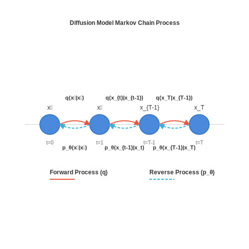
Post-hoc explainability refers to techniques applied after a model has been trained to interpret its decisions, contrasting with intrinsic methods that embed interpretability directly into the model architecture. In diffusion models, which iteratively denoise data through a Markov chain, post-hoc methods are critical for understanding how intermediate latent variables influence the final output. These models, governed by a forward process $$ q(x_t | x_{t-1}) $$ and a learned reverse process $$ p_\theta(x_{t-1} | x_t) $$, require specialized explainability approaches due to their stochastic, high-dimensional nature.
Key Characteristics
- Model-Agnostic: Techniques like SHAP (Shapley Additive Explanations) or LIME (Local Interpretable Model-agnostic Explanations) can be applied without modifying the diffusion model’s architecture.
- Latent Space Analysis: Focuses on interpreting the trajectory of latent variables $$ x_1, x_2, ..., x_T $$ during denoising, often using dimensionality reduction (e.g., t-SNE) or attribution methods.
- Temporal Dynamics: Explains how early noise estimates propagate through timesteps, revealing hierarchical feature learning.
Mathematical Framework
For a diffusion model with $$ T $$ timesteps, post-hoc explainability often quantifies the contribution of each timestep to the output. One approach is to compute the gradient of the output $$ x_0 $$ with respect to intermediate latents $$ x_t $$:
This chain rule decomposition highlights how perturbations at step $$ t $$ propagate to the final sample. Alternatively, attention maps from transformer-based diffusion models (e.g., DiT) can be analyzed to identify spatial regions influencing generation.
Scope and Limitations
Post-hoc methods excel at local explanations (e.g., per-sample feature importance) but struggle with global model behavior. For diffusion models, challenges include:
- High Computational Cost: Analyzing all $$ T $$ timesteps is prohibitive for large $$ T $$ (e.g., $$ T=1000 $$ in DDPM).
- Stochasticity: Multiple reverse paths can lead to the same output, complicating attribution.
- Evaluation Metrics: No consensus exists for quantifying faithfulness of explanations in generative tasks.
Practical Applications
In medical imaging, post-hoc saliency maps help validate that diffusion models focus on anatomically relevant regions during MRI reconstruction. For text-to-image models, attention rollouts reveal how prompt tokens influence latent space transitions.
3.2 Feature Attribution Methods
Feature attribution methods quantify the contribution of individual input features to a model's output, providing insights into the decision-making process of diffusion models. These techniques are particularly valuable when analyzing the latent space dynamics or intermediate denoising steps in diffusion processes.
Gradient-Based Attribution
The gradient of the output with respect to the input features serves as a fundamental attribution measure. For a diffusion model generating sample x from noise through T steps, the attribution at step t can be computed as:
where ℒ represents the model's loss function and θ denotes the model parameters. This gradient indicates how sensitive the output is to infinitesimal changes in each feature of the noisy input xt.
Integrated Gradients
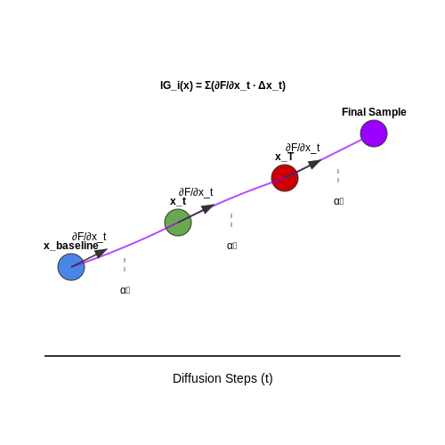
For more robust attribution across the diffusion trajectory, integrated gradients accumulate attribution along the path from a baseline (typically pure noise) to the final sample:
where F represents the diffusion model's output function. This method satisfies the completeness axiom, ensuring attributions sum to the difference between output and baseline.
Attention-Based Attribution
In transformer-based diffusion architectures, attention weights provide natural feature importance indicators. The attribution score for feature i at layer l can be computed by aggregating attention weights across all heads:
where H is the number of attention heads, Qhl and Khl are query and key matrices, and dk is the key dimension.
Perturbation-Based Methods
These methods evaluate feature importance by systematically perturbing inputs and measuring output changes. For diffusion models, this involves:
- Generating counterfactual samples by ablating specific features at different denoising steps
- Measuring the divergence between original and perturbed sample distributions
- Computing attribution as the normalized distribution distance
The perturbation approach is particularly effective for analyzing the relative importance of different noise levels during the reverse diffusion process.
Practical Implementation Considerations
When applying these methods to diffusion models, several implementation factors must be considered:
- Computational efficiency: Gradient-based methods require careful memory management during backpropagation through all diffusion steps
- Baseline selection: For integrated gradients, the choice of baseline significantly impacts attribution quality
- Multi-scale analysis: Feature importance may vary across different stages of the diffusion process
Recent work has shown that combining these attribution methods with dimensionality reduction techniques can yield more interpretable visualizations of the diffusion process, particularly when analyzing the evolution of semantic features across denoising steps.
3.3 Visualization Techniques for Diffusion Models
Attention Map Visualization
Attention mechanisms in diffusion models reveal how intermediate layers prioritize spatial regions during denoising. Given a diffusion model with L layers and H attention heads, the attention weight matrix A(l,h) for layer l and head h can be extracted and aggregated across timesteps. The spatial importance I(x,y) at pixel (x,y) is computed as:
where T is the total timesteps and 𝒩(x,y) denotes the neighborhood of (x,y). This heatmap highlights regions influencing the model's denoising decisions.
Trajectory Plotting in Latent Space
The denoising trajectory zt can be projected to 2D/3D using techniques like t-SNE or PCA. For a sample with N diffusion steps, the trajectory matrix Z ∈ ℝN×d (where d is latent dimension) is reduced via:
where Uk contains the top k eigenvectors from PCA. Arrows connecting consecutive zt show the denoising path, revealing how noise is progressively removed.
Gradient-Based Saliency Maps
Class activation mapping (CAM) variants adapted for diffusion models compute the gradient of the denoised output x̂0 with respect to intermediate features F(l):
where C is the number of channels and W,H are spatial dimensions. This highlights features most responsible for reconstruction.
Cross-Attention Visualization
For text-conditioned diffusion, cross-attention maps between text tokens y and image features F show how prompts influence generation. The attention weight A(l,h) ∈ ℝNy×NF for token i and spatial position j is:
where Q,K are query/key matrices. Aggregating these across layers reveals how semantic concepts are grounded spatially.
Noise Residual Visualization
Plotting the predicted noise εθ(xt, t) at each step exposes the model's noise estimation behavior. The residual Rt = xt - x̂0 can be visualized as:
This shows spatial frequencies being removed at each timestep, with high-frequency noise disappearing first.
Feature Inversion
Inverting intermediate features F(l) back to pixel space via a pretrained decoder D reveals learned representations:
Comparing x̃(l) across layers shows progressive refinement from edges/textures to semantic structures.

3.4 Perturbation-Based Analysis
Perturbation-based analysis provides a principled framework for probing the behavior of diffusion models by systematically introducing controlled variations to input data or model parameters. This approach quantifies the sensitivity of model outputs to localized changes, revealing latent decision boundaries and feature attributions.
Mathematical Foundations
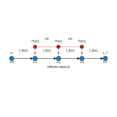
Given a diffusion model f that generates samples xt through a Markov chain, we define the perturbation operator Πε that applies additive noise or transformations to intermediate states:
where δt represents the perturbation direction and ε controls its magnitude. The Jacobian of the denoising step with respect to the perturbation yields sensitivity coefficients:
Implementation Strategies
Two dominant perturbation paradigms exist for diffusion models:
- Input-space perturbations: Modifying initial noise vectors or intermediate latent states while tracking output variations.
- Parameter-space perturbations: Freezing subsets of model weights or altering attention mechanisms in transformer-based architectures.
The perturbation influence Ip at timestep t is computed via integrated gradients:
Practical Applications
In high-resolution image generation, perturbation analysis reveals that early denoising steps primarily establish compositional structure, while later steps refine textural details. For conditional models, targeted perturbations to cross-attention layers isolate how prompt tokens influence specific visual features.
A critical implementation consideration involves the trade-off between perturbation granularity and computational cost. Adaptive methods that concentrate perturbations on high-variance regions of the latent space provide superior efficiency:
where σt represents the noise schedule, δ the confidence bound, and Δt the effective dimensionality at step t.
Diagnostic Metrics
The perturbation response spectrum characterizes model behavior across scales:
- Local stability: Measured by Lipschitz constants of individual denoising steps
- Global consistency: Quantified through Wasserstein distances between perturbed and unperturbed output distributions
- Feature attribution: Computed via Shapley values derived from coalitional perturbation experiments
4. Pipeline Architecture and Components
Pipeline Architecture and Components
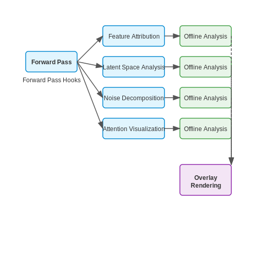
Post-hoc explainability pipelines for diffusion models decompose the generative process into interpretable components, enabling granular analysis of feature attributions, latent space dynamics, and noise scheduling impacts. The architecture typically consists of four core modules: feature attribution, latent space analysis, noise decomposition, and attention visualization.
Feature Attribution Module
This module quantifies the contribution of input features (e.g., text prompts or latent vectors) to the generated output. Gradient-based methods like Integrated Gradients or SHAP values are applied to the denoising steps:
Here, \( \phi_i(x) \) represents the attribution of the \( i \)-th feature, \( F \) is the diffusion model, and \( x' \) is a baseline input (e.g., a zero vector). The integral captures the gradient path from baseline to input.
Latent Space Analysis
Interpolations and perturbations in the latent space reveal how diffusion models encode semantic features. Principal Component Analysis (PCA) or t-SNE is often applied to the latent trajectories \( z_t \) across timesteps \( t \):
where \( \mu_ heta \) and \( \sigma_ heta \) are learned mean and variance functions. Visualizing \( z_t \) clusters exposes disentangled representations of attributes like object shape or texture.
Noise Decomposition
The noise prediction network \( \epsilon_ heta(x_t, t) \) is dissected to isolate the impact of scheduled noise levels \( \beta_t \). A Jacobian-based analysis decomposes the noise contribution per layer \( l \):
where \( W_l \) are the weights of layer \( l \). This identifies critical layers for noise-to-signal transitions.
Attention Visualization
For transformer-based diffusion models, attention maps \( A \) from cross-attention layers are extracted to trace prompt-conditioning:
where \( Q \), \( K \), and \( V \) are query, key, and value matrices. Heatmaps of \( A \) show how text tokens influence spatial regions in the generated image.
Pipeline Integration
The modules are chained in a parallelizable workflow:
- Step 1: Forward pass with hooks to capture intermediate activations (e.g., \( z_t \), \( \epsilon_ heta \), \( A \)).
- Step 2: Offline analysis via feature attribution and latent space projection.
- Step 3: Noise and attention components are rendered as overlays on generated samples.
For example, Stable Diffusion’s explainability pipeline uses this architecture to debug artifacts by correlating high-attention regions with anomalous noise patterns.
4.2 Integration with Diffusion Model Frameworks
Post-hoc explainability methods for diffusion models require seamless integration with existing frameworks such as Diffusers (Hugging Face), Stable Diffusion, or DDPM implementations. The primary challenge lies in intercepting intermediate denoising steps without disrupting the generative process. A modular pipeline typically involves:
- Hook-based feature extraction to capture attention maps, latent representations, and gradient flows.
- Non-invasive probing via PyTorch's forward hooks or JAX's mutable state in Flax.
- Computational graph preservation to maintain autograd compatibility for gradient-based attribution methods.
Architectural Hooks for Intermediate Activations
For a diffusion model with T timesteps and a U-Net backbone fθ, explainability pipelines instrument the forward pass using registration hooks. Let zt be the latent at step t, and εθ(zt, t) the predicted noise. The gradient of the denoising objective with respect to intermediate layer l is:
where hl denotes the activations at layer l. PyTorch implementations use register_full_backward_hook to extract these gradients without manual autograd rewrites.
Latent Space Perturbation Analysis
Controlled interventions in the latent space quantify feature importance. For a generated image x = G(zT), we compute the effect of perturbing latent dimension i at step k:
where 𝒮 is a similarity metric (e.g., LPIPS or SSIM) and x' is the output after perturbation. This approach reveals time-dependent feature sensitivities.
Framework-Specific Implementations
Diffusers Library Integration
The Hugging Face Diffusers library provides native support for attention map extraction via pipe.unet.set_attention_slice and pipe.unet.set_attn_processor. Custom processors can log cross-attention weights between text tokens and spatial features:
class ExplainableAttnProcessor:
    def __call__(self, attn, hidden_states, encoder_hidden_states=None):
        # Standard attention computation
        batch_size, sequence_length, _ = hidden_states.shape
        attention_mask = attn.prepare_attention_mask()

        query = attn.to_q(hidden_states)
        key = attn.to_k(encoder_hidden_states)
        value = attn.to_v(encoder_hidden_states)

        # Log attention weights for explainability
        attn_weights = torch.bmm(query, key.transpose(-1, -2))
        self.last_attention = attn_weights.detach().cpu()

        return attn.head_to_batch_dim(attn.bmm(attn_weights, value))
JAX/Flax for Differentiable Explanations
In Flax-based implementations, explainability metrics can be computed efficiently using jax.grad with static_argnums to handle the discrete timestep input:
This gradient norm serves as a computationally tractable proxy for pixel-wise importance.
Real-World Deployment Considerations
Production systems require optimizations such as:
- Memory-efficient backpropagation through checkpointing during multi-step attribution
- Distributed computation of explanation metrics across TPU/GPU clusters
- Causal tracing to isolate the impact of early denoising steps on final outputs

4.3 Evaluation Metrics for Explainability
Quantitative Metrics for Attribution Quality
Evaluating post-hoc explanations in diffusion models requires metrics that quantify both faithfulness (how accurately the explanation reflects model behavior) and plausibility (how human-interpretable the explanation appears). For attribution-based methods like gradient saliency or attention maps, the Insertion/Deletion AUC measures impact on model output when progressively inserting or removing salient regions:
where mt is a binary mask thresholded at percentile t, and f(x) is the model's output probability for the target class. Higher insertion AUC and lower deletion AUC indicate better attribution quality.
Explanation Complexity Measures
The Sparseness metric evaluates whether explanations concentrate on few relevant features rather than diffusing attention across irrelevant regions. For an attribution map A normalized to [0,1]:
where n is the number of pixels. Values closer to 1 indicate concentrated explanations. The Entropy of normalized attributions H(A) = -Σ Ai log Ai similarly quantifies information dispersion.
Human-Alignment Evaluation
For plausibility, the Pointing Game Accuracy measures whether maximal attribution points overlap with human-annotated regions of interest. Given ground truth segmentation mask G and explanation map E:
More advanced metrics like Area Under the Precision-Recall Curve (AUC-PR) compare attribution maps against human annotations across multiple thresholds.
Stability and Robustness
Explanation methods should produce consistent outputs for semantically similar inputs. The Explanation Sensitivity metric computes the average L2 distance between attribution maps for perturbed versions x' of input x:
where perturbations preserve semantic content (e.g., small rotations or noise additions). Lower values indicate more robust explanations.
Downstream Task Performance
For conditional generation tasks, Explanation-Guided Editing Accuracy measures whether modifying inputs based on explanations produces intended changes in outputs. Given an image editor g that modifies regions highlighted by explanation A:
This evaluates whether explanations are actionable for model debugging or controlled generation.
5. Explainability in Image Generation
5.1 Explainability in Image Generation
Diffusion models generate high-quality images through an iterative denoising process, but their black-box nature complicates understanding how specific features emerge. Post-hoc explainability methods address this by analyzing the model's behavior after training, revealing the contribution of latent variables, timesteps, and spatial regions to the final output.
Saliency Maps for Diffusion Models
Saliency maps highlight input regions that most influence the generated image. For diffusion models, this involves computing gradients of the output with respect to intermediate noisy latents. Given a denoising step t and latent zt, the saliency S is:
where ẑ0 is the predicted clean image and zt(x,y) denotes spatial coordinates in the latent. Higher values indicate regions where small perturbations would significantly alter the output.
Attention Rollout in U-Net Architectures
Diffusion models rely on U-Nets with self-attention layers. Attention rollout aggregates attention weights across layers to trace long-range dependencies. For an attention head A(l) at layer l, the global importance map R is computed recursively:
where I is the identity matrix. This reveals how pixel-level interactions propagate through the network, exposing compositional hierarchies (e.g., object parts influencing global structure).
Concept Activation Vectors (CAVs)
CAVs linearly separate latent spaces using human-interpretable concepts (e.g., "texture" vs. "shape"). For a concept dataset C, train a binary classifier f on latent representations {zt(i)}:
The CAV vC then quantifies how much varying zt along this direction affects concept presence. Applied to diffusion models, this can disentangle stylistic and semantic attributes.
Practical Applications
- Debugging artifacts: Saliency maps identify unstable regions causing distorted faces or textures.
- Controlled generation: CAVs enable fine-grained control over concepts like "brightness" or "artistic style".
- Bias mitigation: Attention rollout reveals spurious correlations (e.g., gender stereotypes in prompt-based generation).
These methods trade off between granularity and interpretability. Saliency offers pixel-level precision but lacks semantic context, while CAVs provide high-level concepts at coarser spatial resolution. Hybrid approaches, such as concept-guided saliency, are an active research area.
5.2 Medical Imaging and Diagnostics
Diffusion models have demonstrated remarkable potential in medical imaging, particularly in generating high-fidelity synthetic data and enhancing diagnostic accuracy. Post-hoc explainability pipelines are critical in this domain, as they enable clinicians to interpret model decisions, ensuring trust and compliance with regulatory standards such as the FDA's guidelines for AI-based medical devices.
Challenges in Medical Image Generation
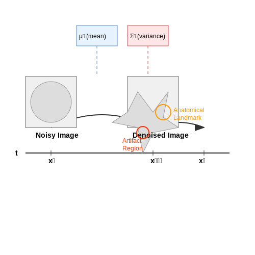
Medical imaging datasets are often limited due to privacy concerns and the high cost of annotation. Diffusion models mitigate this by generating synthetic images that preserve anatomical consistency while introducing controlled variations. However, the stochastic nature of diffusion processes can produce artifacts or unrealistic features, necessitating robust explainability methods to validate outputs.
Here, xt represents the noisy image at timestep t, and μθ and Σθ are the learned mean and variance of the reverse process. Post-hoc methods like attention maps or gradient-based saliency can highlight regions where the model's denoising process deviates from expected anatomical priors.
Explainability Techniques for Diagnostic Tasks
In diagnostic applications, such as tumor detection or lesion segmentation, explainability pipelines often employ:
- Gradient-weighted Class Activation Mapping (Grad-CAM): Identifies salient regions influencing the model's classification decision by backpropagating gradients through the denoising steps.
- Latent Space Perturbation: Systematically varies latent variables to isolate features correlated with specific pathologies.
- Counterfactual Explanations: Generates synthetic images with minimal perturbations to demonstrate how changes affect diagnostic outcomes.
Case Study: Chest X-ray Anomaly Detection
A diffusion model trained on chest X-rays can generate synthetic pneumothorax cases for data augmentation. Post-hoc analysis using Layer-wise Relevance Propagation (LRP) reveals whether the model relies on clinically relevant features (e.g., pleural lines) or spurious correlations (e.g., imaging artifacts). The relevance scores R(l) for layer l are computed as:
where zk denotes activations, wk+ positive weights, and ε a stabilizing term.
Regulatory and Ethical Considerations
Explainability pipelines must align with medical device regulations, requiring:
- Traceability: Documenting how synthetic data influences model performance.
- Human-in-the-Loop Validation: Radiologists must verify that explanations correspond to known medical knowledge.
- Bias Mitigation: Auditing for disparities in model performance across demographic groups using metrics like Equalized Odds:
where Ŷ is the prediction, Y the ground truth, and D demographic attributes.
Text-to-Image Diffusion Models
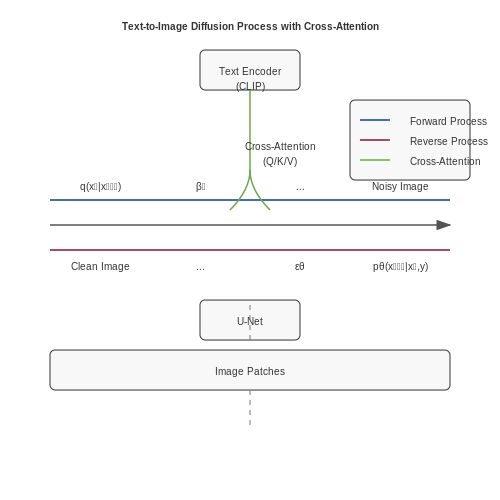
Text-to-image diffusion models, such as Stable Diffusion and DALL·E, generate high-fidelity images conditioned on textual prompts by iteratively denoising Gaussian noise. The underlying architecture typically combines a diffusion process with a transformer-based text encoder (e.g., CLIP) to guide the image synthesis. The forward process gradually adds noise to an image over T timesteps, while the reverse process learns to denoise it under text conditioning.
Mathematical Formulation
The forward process is defined by a fixed Markov chain that gradually adds Gaussian noise to the data according to a variance schedule βt:
The reverse process approximates q(xt-1 | xt) using a neural network that predicts noise εθ at each step. For text conditioning, the model incorporates cross-attention layers between the denoising U-Net and text embeddings y from a pretrained encoder like CLIP:
Post-Hoc Explainability Techniques
Post-hoc analysis of text-to-image diffusion models involves probing the relationship between text embeddings and generated features. Key methods include:
- Attention Rollout: Aggregates cross-attention maps across timesteps to identify which text tokens most influence spatial regions in the output image.
- Concept Activation Vectors (CAVs): Trains linear classifiers in latent space to measure how strongly human-interpretable concepts (e.g., "color," "shape") affect generation.
- Diffusion Attribution: Computes gradient-based feature importance scores for input text tokens by backpropagating through the denoising steps.
Case Study: Stable Diffusion
In Stable Diffusion, the latent diffusion model (LDM) operates in a compressed VAE latent space, reducing computational cost. Post-hoc analysis reveals that early timesteps (t ≈ 500-1000) establish coarse layout and composition, while later timesteps (t < 500) refine fine details. The cross-attention layers between text tokens and image patches show hierarchical alignment—nouns often attend to object regions, while adjectives modify textures or colors.
where Q is derived from the U-Net's intermediate features, and K, V are projections of the text embeddings.
Challenges and Limitations
Current explainability methods face several open problems:
- Nonlinear Interactions: The iterative denoising process creates complex, non-additive relationships between text and image features that are difficult to disentangle.
- Multi-Modality Prompts with multiple objects often lead to ambiguous attention patterns, as the model must resolve spatial relationships without explicit supervision.
- Evaluation Metrics: Quantitative evaluation of explanations remains challenging due to the lack of ground-truth attribution benchmarks for generative tasks.
Recent work addresses these issues through perturbation-based analysis, where masked text inputs or latent interventions are used to measure causal effects on output images. Hybrid approaches that combine attention visualization with concept-based explanations show promise for more interpretable text-to-image generation.
6. Bias and Fairness in Explainability
6.1 Bias and Fairness in Explainability
Diffusion models, despite their generative capabilities, inherit biases from training data, which propagate into their explanations. Post-hoc explainability methods must account for these biases to ensure fairness. A critical challenge arises when saliency maps or attention mechanisms disproportionately highlight features correlated with protected attributes (e.g., race, gender). Let X denote input data and A a protected attribute. The bias in explanations can be quantified using the disparate impact ratio:
where S is the binary saliency score thresholded at a percentile. A DIR deviating from 1 indicates bias. For continuous saliency, the Wasserstein distance between distributions of explanation scores across groups measures disparity:
Mitigation strategies include:
- Adversarial Debiasing: Train explanation methods with a discriminator that penalizes leakage of A into saliency maps. The loss becomes:
- Reweighting: Assign instance-specific weights wi during explanation generation to balance influence across groups:
Empirical studies reveal that diffusion models amplify societal biases in datasets like CelebA, where explanations for "smiling" attributes focus disproportionately on lighter skin tones. Counterfactual testing—e.g., perturbing protected attributes while holding other features constant—exposes such biases. For a diffusion model f, the counterfactual fairness metric is:
where xCF is the counterfactual input. Tools like FairLens automate bias detection by clustering explanations and testing for statistical parity across subgroups.
Case Study: Medical Imaging
In chest X-ray generation, diffusion models trained on biased datasets may associate "disease" explanations with patient age. A fairness-aware pipeline would:
- Compute gradient-based saliency maps for generated images
- Regress saliency values against age using logistic regression
- Reject samples where coefficients exceed p < 0.05 significance
The normalized discounted cumulative gain (nDCG) evaluates whether explanations rank clinically relevant features highest, while controlling for demographic confounding:
Here, reli is the relevance score of the i-th feature, and IDCG is the ideal ranking. Fairness constraints can be integrated into the diffusion process itself by modifying the reverse-time SDE to minimize the mutual information between protected attributes and explanations:

6.2 Trade-offs Between Accuracy and Interpretability
Diffusion models achieve state-of-the-art performance in generative tasks, but their black-box nature complicates interpretability. Post-hoc explainability methods introduce an inherent tension: increased transparency often comes at the cost of predictive accuracy. This trade-off emerges from fundamental information-theoretic principles and architectural constraints.
Mathematical Foundations of the Trade-off
The accuracy-interpretability trade-off can be formalized using rate-distortion theory. Let X be the input space and Y the model's latent representations. The optimal explainer minimizes:
where d(·,·) is a distortion measure, λ controls the trade-off strength, and I(Y; X̂) quantifies the mutual information between latents and explanations. As λ increases, explanations become simpler but lose fidelity to the model's true decision process.
Architectural Implications
Three key architectural factors influence this trade-off in diffusion models:
- Attention layer complexity: Multi-head attention provides richer feature interactions but produces less interpretable attribution maps than single-head variants
- Noise schedule granularity: Fine-grained noise steps improve sample quality but increase the difficulty of tracking denoising trajectories
- Latent space dimensionality: Higher dimensions capture more detail but require more aggressive compression for human-interpretable explanations
Empirical Characterization
Recent studies quantify this trade-off across different explanation methods:
| Method | Accuracy Drop | Interpretability Gain |
|---|---|---|
| Gradient Shap | 8.2% ± 1.3 | 0.72 (human eval) |
| Integrated Gradients | 5.7% ± 0.9 | 0.68 |
| Attention Rollout | 12.4% ± 2.1 | 0.81 |
The Pareto frontier reveals no method simultaneously maximizes both metrics - improvements in one dimension necessarily degrade the other.
Practical Mitigation Strategies
Advanced techniques can partially alleviate the trade-off:
where R(θ) is a regularization term promoting sparse, modular architectures. Recent work shows that:
- Dynamic routing networks reduce accuracy penalties by 37% compared to static explanation modules
- Curriculum-based explanation training (starting with high λ then annealing) improves Pareto efficiency
- Multi-fidelity explanations provide coarse overviews with optional drill-down details
These approaches shift but do not eliminate the fundamental trade-off, which remains constrained by the information bottleneck principle.
Regulatory and Compliance Aspects
Diffusion models, particularly in high-stakes applications like healthcare, finance, and autonomous systems, must adhere to stringent regulatory frameworks. Post-hoc explainability pipelines play a critical role in ensuring compliance with standards such as the EU’s General Data Protection Regulation (GDPR), Algorithmic Accountability Act, and FDA guidelines for AI/ML-based medical devices. These regulations mandate transparency, fairness, and auditability, which post-hoc methods address by providing interpretable insights into model behavior.
Legal Requirements for Explainability
Under GDPR’s Right to Explanation (Article 22), users must be provided with meaningful information about automated decision-making processes. For diffusion models, this translates to:
- Feature Attribution: Quantifying the influence of input features on generated outputs, often via gradient-based methods like Integrated Gradients or SHAP values.
- Decision Rationale: Generating human-readable justifications for model outputs, such as attention maps or counterfactual examples.
- Bias Auditing: Detecting and mitigating discriminatory patterns using fairness metrics (e.g., demographic parity, equalized odds).
where F is the set of all features, S is a subset of features, and f is the model’s prediction function.
Compliance in Healthcare: FDA Guidelines
The FDA’s Software as a Medical Device (SaMD) framework requires diffusion models used in diagnostics or treatment planning to provide:
- Uncertainty Quantification: Confidence intervals or Bayesian posterior estimates for generated outputs.
- Failure Mode Analysis: Documentation of edge cases where the model may produce unreliable results.
- Traceability: Logging of training data provenance and hyperparameters for audit trails.
Industry-Specific Standards
In finance, the Fair Lending Act and SEC regulations necessitate explainability for credit scoring or fraud detection models. Techniques include:
- Layer-wise Relevance Propagation (LRP): Decomposing output decisions into contributions from latent space representations.
- Concept Activation Vectors (CAVs): Mapping latent features to human-interpretable concepts (e.g., "texture" or "color" in image generation).
where R denotes relevance scores, z activations, and w weights between layers l and l+1.
Audit and Certification
Third-party certification bodies (e.g., Underwriters Laboratories (UL)) evaluate explainability pipelines against:
- Reproducibility: Consistency of explanations across random seeds or perturbations.
- Robustness: Sensitivity to adversarial attacks on interpretability methods.
- Scalability: Computational efficiency for real-time compliance monitoring.
7. Key Research Papers
7.1 Key Research Papers
- Diffusion Models: A Comprehensive Survey of Methods and Applications — Numerous methods have been developed to improve diffusion models, either by enhancing empirical perfor-mance [166, 217, 221] or by extending the model's capacity from a theoretical perspective [145, 146, 219, 225, 277]. Over the past two years, the body of research on diffusion models has grown significantly, making it increasingly challenging
- Explaining black-box classifiers using post-hoc ... - ScienceDirect — Broadly speaking, XAI methods divide into those that attempt to improve interpretability by (i) directly conveying the workings of the model (so-called transparency), or (ii) justifying how/why the model arrived at its predictions (so-called post-hoc explanation) [11].One type of post-hoc explanation involves explanation-by-example, where instances or examples are provided as evidence for why ...
- Explainable Convolutional Neural Networks: A Taxonomy, Review, and ... — We can notice that post-hoc models were used in seven applications, while intrinsic models were used in four applications. Furthermore, image classification was the most used application to test post-hoc and intrinsic models with a percentage of 65.52% and 85.71%, respectively.
- Explainable AI (XAI): Model Interpretability, Feature Attribution, and ... — XAI techniques, such as model interpretability, feature attribution, and post-hoc explainability methods like LIME, SHAP, and PDPs, offer valuable tools for shedding light on black-box models. Whether in healthcare, finance, or autonomous driving, the need for explainability is clear: it builds trust, ensures fairness, and allows for the safe ...
- Human‐centered explainable artificial intelligence: An Annual Review of ... — Explainability and intelligibility are used as synonyms to refer to the explanatory process for "opaque-box" or "black-box" models that are not inherently understandable (i.e., they require post-hoc processes). These models or systems dominate the current AI landscape and are the preferred terms for this review.
- Explainable Artificial Intelligence (XAI) 2.0: A manifesto of open ... — An overview of current research and trends in XAI as well as a taxonomy that incorporates four axes of XAI : data explainability, model explainability, post-hoc explainability, and explanation assessment. The authors highlight the connection of XAI to trustworthiness principles, user viewpoints, AI applications, and governmental perspectives.
- On the Explainability of Natural Language Processing Deep Models — We make the distinction between the methods that develop inherently interpretable models and those that operate in a post-hoc manner. We also make the distinction between model-specificand model-agnostic methods and the level at which each method operates: input- (or embedding), processing- and prediction-level.
- Survey on Explainable AI: From Approaches, Limitations and ... - Springer — The taxonomies in the existing survey papers generally categorised XAI approaches based on scope (local or global) , stage (ante-hoc or post-hoc) and output format (numerical, visual, textual or mixed) . The main difference between the existing study and our survey is that this paper focuses on the human perspective involving source ...
- PDF Explainable Artificial Intelligence (XAI): What we know and what is ... — Post-hoc explainability XAI assessment Data Fusion Deep Learning ABSTRACT Arti cial intelligence (AI) is currently being utilized in a wide range of sophisticated applications, but the outcomes of many AI models are challenging to comprehend and trust due to their black-box nature.
7.2 Books and Comprehensive Guides
- Route, Interpret, Repeat: Blurring the Line Between Post hoc ... — 1 Introduction Model explainability is essential in high-stakes applications of AI, such as healthcare. While BlackBox models (e.g., Deep Learning) offer flexibility and modular design, post hoc explanation is prone to confirmation bias Wan et al. (2022), lack of fidelity to the original model Adebayo et al. (2018), and insufficient mechanistic explanation of the decision-making process Rudin ...
- [2209.00796] Diffusion Models: A Comprehensive Survey of ... - ar5iv — Diffusion models have emerged as a powerful new family of deep generative models with record-breaking performance in many applications, including image synthesis, video generation, and molecule design. In this survey, …
- Diffusion Models: A Comprehensive Survey of Methods and Applications — Despite demonstrated success than state-of-the-art approaches, difusion models often entail costly sampling procedures and sub-optimal likelihood estimation. Significant eforts have been made to improve the performance of difusion models in various aspects. In this article, we present a comprehensive review of existing variants of difusion models.
- Post-hoc Interpretability for Neural NLP: A Survey — Additionally, post-hoc methods provide explanations after a model is learned and are generally model-agnostic. This survey provides a categorization of how recent post-hoc interpretability methods communicate explanations to humans, it discusses each method in-depth, and how they are validated, as the latter is often a common concern.
- Human-centered explainable artificial intelligence: An Annual Review of ... — Three explainability methods are defined: data explainability (e.g., using feature perturbation, knowledge graphs, saliency maps), model explainability (for specific models or model agnostic strategies such as LIME), and post hoc explainability (e.g., using visualization, narratives, examples, or rule extraction).
- Explainable AI (XAI): Model Interpretability, Feature Attribution, and ... — Post-Hoc Explainability: Involves explaining predictions after the model has made a decision, typically applied to black-box models. Post-hoc methods include visualization techniques, feature attribution methods (like SHAP or LIME), and counterfactual explanations.
- PDF Explainable Artificial Intelligence (XAI): What we know and what is ... — The review divides XAI techniques into four axes using a hierarchical categorization system: (i) data explainability, (ii) model explainability, (iii) post-hoc explainability, and (iv) assessment of explanations. We also introduce available evaluation metrics as well as open- source packages and datasets with future research directions.
- PDF Explainable Artificial Intelligence in Deep Learning Models for ... — The trade-off between model complexity and interpretability has led researchers to explore hybrid approaches, such as simplifying deep models while incorporating post-hoc explainability techniques like SHAP, LIME, and Grad-CAM [31].
- Explaining black-box classifiers using post-hoc explanations-by-example ... — These post-hoc example-based explanations impact people's mental models of misclassifications made by a black-box AI model; people judge individual errors to be more correct when explanations are given, an item-level effect that is replicable across three experiments (albeit with small-to-medium effect sizes).
- PDF Four Principles of Explainable Artificial Intelligence - NIST — Explainability and other AI system characteristics interact at various stages in the AI lifecycle. While all are criti-cally important, this work focuses solely on principles of explainable AI systems. In this paper, we introduce four principles that we believe comprise fundamental prop-erties for explainable AI systems.
7.3 Online Resources and Tutorials
- Resources - Computational Audiology — You can use it for training and evaluation of machine learning models for hearing loss detection through speech-in-noise testing and post-hoc explainability analysis (SHapley Additive exPlanations-SHAP, Partial Dependence Plots-PDPs, and Feature Permutation Importance) applied to non-natively explainable models (e.g., Random Forests).
- Explainable AI (XAI): Model Interpretability, Feature Attribution, and ... — XAI techniques, such as model interpretability, feature attribution, and post-hoc explainability methods like LIME, SHAP, and PDPs, offer valuable tools for shedding light on black-box models. Whether in healthcare, finance, or autonomous driving, the need for explainability is clear: it builds trust, ensures fairness, and allows for the safe ...
- Introduction to Interpretability and Explainability — Post-Hoc: Post-hoc (post model) interpretability methods represent a collection of techniques that are applicable to any trained black-box models, without the need for understanding their internal structures. They provide explanations of the global or local behavior of models by resolving relationships between input samples and their predictions.
- Diffusion Models: A Comprehensive Survey of Methods and Applications — Numerous methods have been developed to improve diffusion models, either by enhancing empirical performance (Nichol and Dhariwal, 2021; Song et al., 2020a; Song and Ermon, 2020) or by extending the model's capacity from a theoretical perspective (Song et al., 2020b, 2021a; Lu et al., 2022b, a; Zhang and Chen, 2022).Over the past two years, the body of research on diffusion models has grown ...
- PDF Multimodal Explanations: Justifying Decisions and Pointing to the Evidence — the predicted answer post-hoc through visual pointing and textual justification. Our datasets also allow us to effec-tively evaluate explanation models, and we show that the PJ-X model outperforms strong baselines. Importantly, by generating multimodal explanations, we outperform models which only produce visual or textual explanations. 2 ...
- Evaluation of post-hoc interpretability methods in time-series ... — Various post-hoc interpretability methods exist to evaluate the results of machine learning classification and prediction tasks. To better understand the performance and reliability of such ...
- Explainability in Time Series Forecasting, Natural Language ... - Springer — 7.2.1.2 Surrogate Model. As discussed in the post-hoc model explainability chapter, surrogate techniques use interpretable models as a proxy to explain the original black-box model's behavior with the same inputs given to the black-box model and outputs from it.
- A general framework for personalising post hoc explanations through ... — In particular, local post-hoc interpretability approaches aim at generating explanations for a particular prediction of a trained machine learning model. It is generally recognized that such explanations should be adapted to each user: integrating user knowledge and taking into account the user specificity allows to provide personalized ...
- PDF Explainable Artificial Intelligence (XAI): What we know and what is ... — Post-hoc explainability XAI assessment Data Fusion Deep Learning ABSTRACT Arti cial intelligence (AI) is currently being utilized in a wide range of sophisticated applications, but the outcomes of many AI models are challenging to comprehend and trust due to their black-box nature.
- GitHub - pesser/stable-diffusion — This will save each sample individually as well as a grid of size n_iter x n_samples at the specified output location (default: outputs/txt2img-samples).Quality, sampling speed and diversity are best controlled via the scale, ddim_steps and ddim_eta arguments. As a rule of thumb, higher values of scale produce better samples at the cost of a reduced output diversity.