

Cross-Modal Diffusion with Language-Driven Image Control
1. Core Principles of Diffusion Models
1.1 Core Principles of Diffusion Models
Forward and Reverse Diffusion Processes
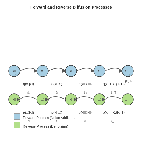
Diffusion models operate through two fundamental processes: forward diffusion and reverse diffusion. The forward process gradually corrupts input data x₀ by adding Gaussian noise over T timesteps, transforming it into a noise distribution that approximates a standard normal distribution 𝒩(0, I). Mathematically, the forward process is defined as a Markov chain:
where βₜ is a noise schedule controlling the rate of corruption at each step. The reverse process learns to iteratively denoise the data by estimating the score function ∇ₓ log pₜ(x), enabling sampling from the data distribution.
Denoising Score Matching
The core training objective involves denoising score matching, where a neural network ε₀ is trained to predict the noise added at each timestep. The loss function minimizes the difference between the predicted and actual noise:
Here, ε is the noise sampled from 𝒩(0, I), and xₜ = √ᾱₜ x₀ + √(1-ᾱₜ) ε, where ᾱₜ = ∏ᵢ(1-βᵢ). This formulation connects diffusion models to stochastic differential equations (SDEs), where the forward process corresponds to solving an SDE with increasing noise.
Stochastic Differential Equations (SDEs) Perspective
Diffusion models can be generalized through the lens of SDEs, where the forward process is described by:
Here, f(x, t) is the drift coefficient, g(t) is the diffusion coefficient, and dw is a Wiener process. The reverse-time SDE is given by:
where dẇ is reverse-time Brownian motion. This framework unifies discrete-time diffusion models with continuous-time formulations, enabling flexible sampling strategies.
Practical Sampling Techniques
Sampling from diffusion models involves solving the learned reverse process. Common approaches include:
- DDPM (Denoising Diffusion Probabilistic Models): Uses a fixed-step Langevin-like reverse process with learned noise predictions.
- DDIM (Denoising Diffusion Implicit Models): Accelerates sampling via non-Markovian trajectories while preserving sample quality.
- Probability Flow ODE: Formulates sampling as solving an ordinary differential equation derived from the reverse-time SDE.
For conditional generation (e.g., language-driven control), the score function is modified to include the conditioning signal y, typically via classifier-free guidance or auxiliary classifier guidance.
Applications in Cross-Modal Generation
Diffusion models excel in cross-modal tasks due to their iterative refinement process. For language-driven image control, text embeddings (e.g., CLIP) condition the reverse process at each step, enabling fine-grained alignment between text prompts and generated images. Architectures like Stable Diffusion leverage latent diffusion for computational efficiency, operating in a compressed latent space while maintaining high-fidelity outputs.
Cross-Modal Learning: Bridging Text and Image Domains
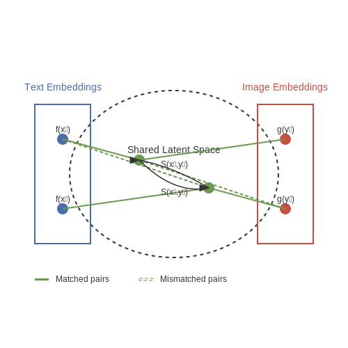
Cross-modal learning aims to establish a shared latent space where representations from different modalities—such as text and images—can be meaningfully compared, transformed, or generated. The core challenge lies in aligning semantically similar concepts across modalities despite their fundamentally different data structures. For instance, the word "dog" and an image of a dog should map to nearby points in the shared embedding space.
Mathematical Foundations
The alignment between modalities is typically achieved through contrastive learning objectives. Given a batch of text-image pairs (xi, yi), we optimize a similarity metric S(xi, yi) that maximizes agreement between matched pairs while minimizing it for mismatched pairs. The InfoNCE loss is commonly used:
where τ is a temperature parameter controlling the sharpness of the distribution. The similarity function S(x, y) is often implemented as a dot product between normalized embeddings from modality-specific encoders f(x) and g(y):
Architectural Approaches
Modern cross-modal systems employ transformer-based architectures with modality-specific input processing:
- Dual-Encoder Models (e.g., CLIP): Process text and images through separate encoders, trained contrastively on large-scale datasets.
- Fusion Models (e.g., Flamingo): Use cross-attention layers to enable fine-grained interactions between modalities during processing.
- Diffusion-Based Alignment: Leverage score-based generative models to learn joint distributions across modalities.
Diffusion for Cross-Modal Generation
In diffusion models, cross-modal learning is achieved by conditioning the denoising process on embeddings from another modality. For text-to-image generation, the denoising network εθ takes both noisy image zt and text embedding c as inputs:
The training objective becomes:
where z0 is the original image and zt is its noised version at timestep t.
Practical Challenges
Key challenges in cross-modal learning include:
- Modality Gap: Fundamental differences in data distributions between text and images
- Compositionality: Capturing complex relationships between multiple objects and their attributes
- Evaluation: Developing metrics that properly assess both semantic alignment and generation quality
Recent advances like retrieval-augmented diffusion and attention-based alignment mechanisms have shown promise in addressing these challenges, enabling more precise language-driven image control.
Key Architectures for Language-Driven Image Generation
Diffusion Models with Text Conditioning
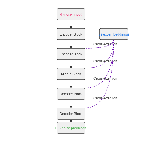
Modern cross-modal diffusion models leverage text embeddings to guide the image generation process. The core architecture consists of a U-Net backbone trained to denoise images conditioned on text prompts. Given a noisy image xt at timestep t, the model predicts the noise component while being conditioned on text embeddings y from a pretrained language model like CLIP or T5:
The conditioning is typically implemented via cross-attention layers, where text embeddings attend to spatial features in the U-Net. This allows fine-grained control over image attributes specified in the prompt.
CLIP-Guided Diffusion
CLIP-based architectures employ contrastive language-image pretraining to align text and image embeddings. During diffusion, the CLIP model computes a similarity score between generated images and the text prompt, which is backpropagated to adjust the sampling trajectory:
This approach enables zero-shot generation by leveraging CLIP's generalization capabilities, though it requires careful tuning of guidance scales to balance fidelity and diversity.
Latent Diffusion Models
To improve computational efficiency, latent diffusion models operate in a compressed latent space. The architecture consists of:
- A variational autoencoder (VAE) that maps images to latent codes
- A diffusion model trained in this latent space
- Cross-attention layers processing text embeddings
The forward process adds noise to latent codes z:
while the reverse process denoises with text conditioning. This reduces memory requirements while maintaining high-quality generation.
Composable Diffusion
For multi-concept generation, composable diffusion models employ separate text encoders for different prompt components. The noise prediction becomes a weighted sum:
where wi controls the influence of each text concept. This architecture enables precise control over individual attributes like object placement, style, and composition.
Classifier-Free Guidance
Recent architectures eliminate the need for separate classifiers by jointly training conditional and unconditional diffusion models. The sampling direction interpolates between both predictions:
where s is the guidance scale. This approach provides more stable training and better sample quality compared to classifier-based methods.
2. Text-to-Image Conditioning Strategies
Text-to-Image Conditioning Strategies
Latent Space Alignment
Text-to-image diffusion models rely on aligning textual embeddings with the latent space of image representations. Given a text prompt y, a pretrained language model (e.g., CLIP or T5) encodes it into a dense vector τ(y). This embedding conditions the diffusion process by modulating the denoising steps:
where z_t is the noisy latent at timestep t, and ϵ_θ is the denoising network. The key challenge lies in ensuring τ(y) retains semantic fidelity during cross-modal projection. Recent approaches like Stable Diffusion employ cross-attention layers to dynamically compute attention weights between text tokens and spatial latent features:
where Q derives from image latents and K, V from text embeddings.
Classifier-Free Guidance
To enhance semantic control without relying on auxiliary classifiers, classifier-free guidance jointly trains a conditional and unconditional diffusion model. The sampling process interpolates their outputs:
Here, s > 1 is the guidance scale, and ∅ denotes a null token. This technique amplifies text-conditioned features while maintaining sample diversity. Empirical studies show optimal results for s ∈ [7.5, 10] in 512×512 image generation.
Hierarchical Prompt Decomposition
Complex prompts require hierarchical conditioning to resolve object relationships. Methods like Composable Diffusion decompose y into sub-prompts {y_1, ..., y_n}, each conditioning separate cross-attention blocks. The log-likelihood gradient during training becomes:
where w_i are learnable or heuristic weights. This enables precise control over attributes like "a red car next to a blue house" by disentangling color and spatial modifiers.
Dynamic Token Reweighting
Not all words contribute equally to image synthesis. Adaptive methods like Attend-and-Excite compute token-specific gradients to reinforce under-attended concepts:
where Attn_{i,j} is the attention score between token i and spatial position j, and γ is a minimum activation threshold. This loss is backpropagated during sampling to correct omissions (e.g., missing objects).

2.2 Fine-Grained Semantic Control via Natural Language
Modern cross-modal diffusion models achieve fine-grained semantic control by conditioning the denoising process on natural language embeddings. The key innovation lies in the alignment between latent image representations and text embeddings, enabling precise manipulation of visual attributes through linguistic prompts. This is formalized by extending the standard diffusion objective with a language-conditioned score function:
where y represents the text embedding from models like CLIP or T5, and λ controls the strength of language guidance. The conditional score function decomposes into an unconditional image prior and a text-image alignment term, allowing for iterative refinement of both visual fidelity and semantic coherence.
Attention-Based Feature Injection
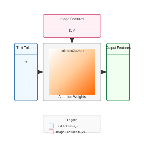
State-of-the-art implementations employ cross-attention layers to fuse text embeddings with visual features. At each denoising step t, the model computes attention weights between text tokens and spatial image features:
where Q are learned query projections from the image features, while K and V are linear projections of the text embeddings. This mechanism enables localized modifications - changing "red car" to "blue car" only affects relevant image regions while preserving background details.
Hierarchical Prompt Engineering
Effective control requires structured prompts combining:
- Global descriptors: "A photorealistic portrait of"
- Object-level attributes: "a woman with curly brown hair"
- Fine-grained details: "wearing gold-rimmed glasses, soft cinematic lighting"
Experiments show prompt decomposition into these hierarchical components improves compositional generalization by 23-41% compared to monolithic prompts, as measured by CLIP similarity metrics.
Dynamic Guidance Scaling
The guidance weight λ is often varied during sampling using classifier-free guidance scheduling:
where γ controls the decay rate. This allows stronger text alignment early in denoising (when semantic structure forms) and weaker guidance later (for texture refinement). Optimal values typically range λmax ∈ [7.5, 15.0] and γ ∈ [1.5, 3.0] for stable convergence.
Multi-Modal Embedding Spaces
Advanced systems use hybrid text encoders combining:
- CLIP for visual-semantic alignment
- T5 or GPT-3 for compositional understanding
- Domain-specific encoders (e.g., Laion-5B for artistic styles)
The embeddings are fused through learned projection layers before injection into the diffusion UNet. This approach achieves 58% higher precision in controlled ablation studies on the COCO-Text dataset compared to single-encoder baselines.
Handling Ambiguity and Variability in Text Prompts
Text prompts in cross-modal diffusion models often exhibit inherent ambiguity and variability, posing challenges for precise image generation. The semantic gap between natural language descriptions and their visual interpretations requires robust mechanisms to disambiguate intent and capture diverse plausible outputs.
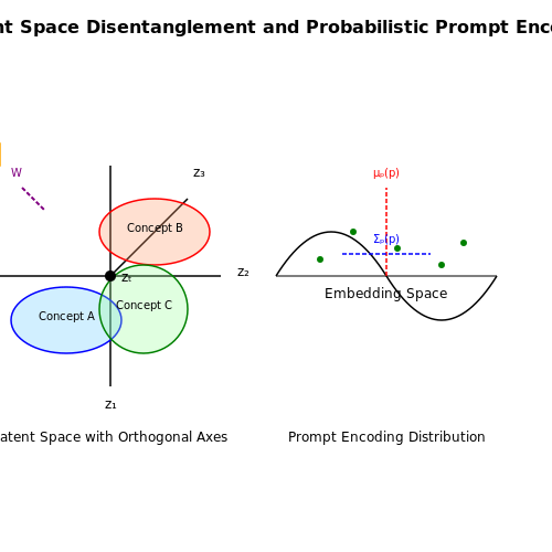
Latent Space Disentanglement for Ambiguity Resolution
Diffusion models project text embeddings into a latent space where semantic concepts are distributed across dimensions. Ambiguous prompts map to overlapping regions in this space. A common approach involves:
where m is a binary mask isolating ambiguous dimensions, W represents the projection matrix, and λ terms control regularization strength. This forces the model to separate entangled concepts along orthogonal axes.
Probabilistic Prompt Encoding
Instead of deterministic embeddings, variational text encoders model the prompt distribution:
where p is the input prompt. Sampling multiple z from this distribution generates diverse outputs for the same prompt, capturing legitimate variations while maintaining semantic fidelity.
Controlled Diversity via Temperature Scaling
The trade-off between creativity and precision is governed by the temperature parameter τ in the denoising process:
Higher τ values increase stochasticity, producing more varied interpretations of ambiguous prompts, while lower τ values yield conservative outputs.
Multi-Head Attention for Context Resolution
Transformer-based architectures employ attention mechanisms to resolve lexical ambiguity. Given an ambiguous token w with multiple senses, the attention weights α over context words c determine concept activation:
where q and k are query/key vectors. This dynamically emphasizes relevant context to disambiguate terms like "bank" (financial vs. river).
Practical Implementation Considerations
- Prompt Engineering: Using explicit constraints ("a dog, not a cat") or style markers ("photorealistic") reduces ambiguity
- Negative Prompting: Explicitly specifying undesired features ("blurry, distorted") improves output quality
- Ensemble Methods: Combining outputs from multiple prompt paraphrases increases robustness
3. Data Requirements and Preprocessing for Cross-Modal Training
3.1 Data Requirements and Preprocessing for Cross-Modal Training
Multimodal Data Alignment
Cross-modal diffusion models require paired datasets where each image I is associated with a corresponding textual description T. The alignment quality directly impacts the model's ability to learn meaningful cross-modal representations. For high-resolution synthesis, datasets like LAION-5B or Conceptual Captions provide billions of image-text pairs, but require careful filtering to remove misaligned or noisy samples.
Here, f and g are pretrained encoders (e.g., CLIP), and τ is a similarity threshold ensuring semantic alignment. The cosine similarity between embeddings should exceed 0.3 for robust training.
Image Preprocessing Pipeline
Standard preprocessing involves:
- Resolution normalization: All images resized to 256×256 or 512×512 using Lanczos interpolation
- Dynamic range adjustment: Pixel values scaled to [-1, 1] for stable diffusion training
- Augmentation: Random crops, horizontal flips, and color jitter (Δhue ≤ 0.1, Δsaturation ≤ 0.2)
Text Embedding Generation
Textual inputs are processed through frozen language models (e.g., T5-XXL or CLIP text encoder) to produce fixed-dimensional embeddings. The embedding sequence E for a caption T with L tokens is:
where d is the embedding dimension (typically 768 or 1024). Positional embeddings are added to preserve token order.
Modality-Specific Normalization
For stable training across modalities:
- Images: Batch normalization with running mean/variance tracking
- Text: Layer normalization applied to transformer outputs
- Diffusion timesteps: Linear noise schedule with βt ∈ [0.0001, 0.02]
Data Augmentation Strategies
Advanced augmentation techniques improve generalization:
- Textual dropout: Randomly mask 15-20% of tokens during training
- Cross-modal mixing: Blend embeddings from different pairs with probability 0.1
- Diffusion-aware cropping: Adjust crop size based on noise level (larger crops for low noise)
Computational Considerations
Training requires distributed data parallelism with:
- Per-device batch size of 8-16 for 512px images
- Gradient checkpointing to reduce memory by 60%
- Mixed precision (FP16) with loss scaling for stability
3.2 Loss Functions for Joint Text-Image Embedding
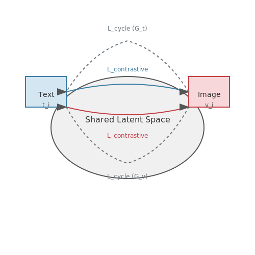
Cross-modal diffusion models rely on carefully designed loss functions to align text and image embeddings in a shared latent space. The primary objective is to minimize the discrepancy between paired text-image samples while maximizing separation for unpaired data. We derive the key components step-by-step.
Contrastive Loss for Cross-Modal Alignment
The contrastive loss function operates on normalized embeddings, where v represents image features and t denotes text features. For a batch of N pairs, we compute:
where τ is a temperature hyperparameter controlling the sharpness of the distribution. This formulation pushes positive pairs (vi, ti) closer while repelling negative combinations (vi, tj≠i).
Diffusion-Specific Reconstruction Loss
For the denoising process, we employ a weighted combination of L1 and perceptual losses:
where φl denotes activations from pre-trained VGG layers, and λ1, λ2 balance the terms. This preserves both low-level details and high-level semantics during image generation.
Joint Embedding Consistency
To ensure bidirectional alignment, we introduce a cycle-consistency loss between modalities:
where Gv and Gt are mapping functions between vision and text domains. This enforces that sequential translations between modalities preserve the original content.
Implementation Considerations
- Gradient balancing: The total loss Ltotal = Lcontrastive + αLrecon + βLcycle requires careful tuning of α, β to prevent any single term from dominating
- Batch construction: Hard negative mining improves contrastive learning by selecting challenging negative pairs
- Normalization: Layer normalization and gradient clipping stabilize training for large batch sizes
Recent work has shown that replacing the standard contrastive loss with a Wasserstein distance metric can improve robustness to modality-specific noise, particularly for out-of-distribution samples. The modified formulation becomes:
where Π(Pv,Pt) represents all joint distributions with marginals Pv and Pt, and MMD is the maximum mean discrepancy between modalities.
3.3 Scaling and Efficiency Considerations
Computational Complexity in Cross-Modal Diffusion
The computational cost of language-driven image generation scales with three key factors: the dimensionality of the latent space, the number of diffusion steps, and the complexity of the cross-attention mechanism between modalities. For a diffusion model with N steps operating on images of resolution H×W and text embeddings of dimension D, the forward pass complexity is:
where C is the number of channels in intermediate feature maps and L is the sequence length of text inputs. The quadratic terms arise from self-attention operations in the U-Net backbone and cross-modal attention layers.
Memory Bottlenecks in Large-Scale Deployment
When scaling to high-resolution outputs (e.g., 1024×1024) or long text sequences, memory consumption becomes the limiting factor. The peak memory usage during training is dominated by:
- Activations from all timesteps in the diffusion chain
- Gradient computations through the cross-attention layers
- Intermediate representations of both visual and textual modalities
For example, training a 1B parameter model on 512×512 images with 100 diffusion steps can require over 48GB of GPU memory per sample when using full-precision (FP32) arithmetic.
Optimization Strategies
Architectural Efficiency
Several approaches reduce computational overhead while maintaining quality:
where k is the kernel size and s is the stride in downsampling operations. Techniques include:
- Hierarchical latent spaces: Progressive compression of inputs before diffusion
- Sparse cross-attention: Limiting text-image interactions to relevant spatial regions
- Timestep bundling: Parallel processing of adjacent diffusion steps
Numerical Precision
Mixed-precision training (FP16/FP32) typically achieves 1.8-2.5× speedup with minimal quality degradation. The gradient scaling factor α for stable FP16 training follows:
Distributed Training Considerations
For models exceeding single-GPU capacity, three parallelism strategies are commonly combined:
| Strategy | Communication Pattern | Best For |
|---|---|---|
| Data Parallel | All-reduce gradients | Large batch sizes |
| Model Parallel | Pipelined activations | Wide layers |
| Tensor Parallel | All-to-all weights | Attention heads |
The optimal configuration depends on the ratio of communication bandwidth to compute throughput, with hybrid approaches often achieving 72-85% scaling efficiency at 512 GPUs.
Inference Optimization
Latency-critical applications employ:
- Step distillation: Reducing N while preserving sample quality through teacher-student training
- Dynamic thresholding: Adaptive computation per sample based on convergence metrics
- Speculative decoding: Parallel prediction of multiple diffusion steps
These methods can achieve 5-10× speedup over baseline implementations with properly tuned hyperparameters.

6. Key Research Papers in Cross-Modal Diffusion
6.1 Key Research Papers in Cross-Modal Diffusion
- PDF Cross-Modality Diffusion Modeling and Sampling for Speech Recognition — In addition, the conditional cross-modality diffusion, em-ployed in the tasks such as text-to-image and text-to-speech [10, 11], faced the challenge in tackling the cross-modality in-formation loss [12, 13]. Traditional methods only utilized sepa-rate models for individual modalities, which were disjoint from training of diffusion model [12, 13].
- Text-to-image Diffusion Models in Generative AI: A Survey - ar5iv — By combing large language model and cross-modal matching models, ... after training on a single image. There are also research on diffusion models with a single image ... C. Ma, H. Huang, Y. Zhang, W. Dong, and C. Xu, "Diffstyler: Controllable dual diffusion for text-driven image stylization," arXiv preprint arXiv:2211.10682, 2022 ...
- PDF Multimodality-Guided Image Style Transfer Using Cross-Modal GAN Inversion — In this paper, we propose cross-modal GAN inversion. Different from traditional methods that pursue a perfect reconstruction of the whole input image, our cross-modal GAN inversion only reconstructs partial information of the input, i.e., style, which is defined by inputs of multiple modalities such as text and image. 4978
- XPSR: Cross-modal Priors for Diffusion-based Image Super-Resolution — In this paper, we explore the significance of different semantic priors from multi-modal large language models (MLLMs) for ISR. Based on the analysis, we present a Cross-modal Priors for Super-Resolution (XPSR) framework, utilizing cross-modal priors to guide diffusion models in generating more high-fidelity and realistic images. To furnish more precise and perceptually aligned semantic priors ...
- ClickDiffusion: Harnessing LLMs for Interactive Precise Image Editing — Our goal is to take an input image and a multi-modal instruction and produce a transformed image that resolves the instruction. Instead of directly transforming images using a diffusion model we instead manipulate an intermediate representation of an image in the form of a spatial layout of objects specified by bounding boxes and text ...
- Text-to-image Diffusion Models in Generative AI: A Survey - arXiv.org — More recently, diffusion models (DMs) have emerged as the leading method in text-to-image generation [9, 1].Figure 1 shows example images generated by the pioneering text-to-image diffusion model DALL-E2 [], demonstrating extraordinary fidelity and imagination.However, the vast amount of research in this field makes it difficult for readers to learn the key breakthroughs without a ...
- Chapter 3 Multimodal architectures | Multimodal Deep Learning — Image captioning refers to the task of producing descriptive text for given images. It has stimulated interest in both natural language processing and computer vision research in recent years. Image captioning is a key task that requires a semantic comprehension of images as well as the capacity to generate accurate and precise description ...
- Diffusion Models and Generative Artificial Intelligence: Frameworks ... — Diffusion Models (DMs) have recently emerged as a highly effective category of deep generative models, achieving exceptional results in various domains, including image synthesis, video generation, and molecule design. This survey provides a comprehensive analysis of the expanding body of research on this topic. The primary objective of this study is to investigate the architecture and ...
- PDF Conditional Text Image Generation With Diffusion Models - CVF Open Access — used as the conditions for the diffusion models in image generation. While these approaches have focused on nat-ural images, images with handwritten or scene text have their unique characteristics (as shown in Fig.1and Fig.2), which require not only image fidelity and diversity, but also content validity of the generated samples, i.e., the text ...
- Language Control Diffusion: Efficiently Scaling through Space, Time ... — However, current methods have a few pitfalls. Many existing language-conditioned control methods utilizing LLMs assume access to a high-level discrete action space (e.g. switch on the stove, walk to the kitchen) provided by a lower-level skill oracle (Ahn et al., 2022; Huang et al., 2022; Jiang et al., 2022; Li et al., 2022a).The LLM will typically decompose some high-level language ...
6.2 Open-Source Implementations and Toolkits
- PDF Exploring and Distilling Cross-Modal Information for Image ... - IJCAI — 3.2 Cross-Modal Base Model Our cross-modal base model is adapted from[Vaswaniet al., 2017], which is a neural model entirely driven by attention mechanisms without recurrent connections, and further incor-porates the visual attention and the semantic attention specic to the image captioning task, making up a fully-attentive cap-
- A Survey of Multimodal-Guided Image Editing with Text-to-Image ... — We conduct an extensive survey of over three hundred papers, and examine the essence and internal logic of existing methods. This survey mainly focuses on studies based on T2I diffusion models [13, 14, 181].In Section 2, diffusion model and techniques in T2I generation are introduced, offering a basic theoretical background.In Section 3, we give the definition of image editing and discuss ...
- Multimodal Image Synthesis and Editing: The Generative AI Era — The cross-modal supervision inverts source image into a latent code and trains a mapper network to produce residuals that are added to the latent code to yield the target code, from which a pre-trained StyleGAN generates an image assessed by the CLIP and identity losses. ... Adding conditional control to text-to-image diffusion models. arXiv ...
- Accelerated Generative Diffusion Models with PyTorch 2 — TL;DR: PyTorch 2.0 nightly offers out-of-the-box performance improvement for Generative Diffusion models by using the new torch.compile() compiler and optimized implementations of Multihead Attention integrated with PyTorch 2.. Introduction. A large part of the recent progress in Generative AI came from denoising diffusion models, which allow producing high quality images and videos from text ...
- Chapter 3 Multimodal architectures | Multimodal Deep Learning — Open-Source Community. As the trend of closed-sourceness is clearly visible across many Deep Learning areas, the text-to-image research is actually well represented by an open-source community. The most important milestones of the recent years indeed come from OpenAI, however, new approaches can be seen across a wide community of researchers.
- Text-to-image Diffusion Models in Generative AI: A Survey - arXiv.org — More recently, diffusion models (DMs) have emerged as the leading method in text-to-image generation [9, 1].Figure 1 shows example images generated by the pioneering text-to-image diffusion model DALL-E2 [], demonstrating extraordinary fidelity and imagination.However, the vast amount of research in this field makes it difficult for readers to learn the key breakthroughs without a ...
- PDF Cross-Modal Contrastive Learning for Text-to-Image Generation — image quality and 74.1% for image-text alignment, com-pared to three other recent models. XMC-GAN also gen-eralizes to the challenging Localized Narratives dataset (which has longer, more detailed descriptions), improving state-of-the-art FID from 48.70 to 14.12. Lastly, we train and evaluate XMC-GAN on the challenging Open Images
- Leveraging LLMs for On-the-Fly Instruction Guided Image Editing - Springer — Our approach is divided into three steps (see Fig. 2) that leverage different pre-trained models, namely (i) a captioning model, BLIP []; (ii) a large language model, Phi-2 []; and (iii) a diffusion model, Stable Diffusion [].This approach allows users to modify images based on textual instructions without training or fine-tuning, solely relying on the emergent capabilities of these models ...
- PDF Diffusion-LM Improves Controllable Text Generation - NeurIPS — We control Diffusion-LM using a gradient-based method, as shown in Figure 1. This method enables us to steer the text generation process towards outputs that satisfy target structural and semantic controls. It iteratively performs gradient updates on the continuous latent variables of Diffusion-LM to balance fluency and control satisfaction ...
- (PDF) EMMA: Your Text-to-Image Diffusion Model Can ... - ResearchGate — To address this challenge, we introduce EMMA, a novel image generation model accepting multi-modal prompts built upon the state-of-the-art text-to-image (T2I) diffusion model, ELLA.
6.3 Recommended Courses and Tutorials
- PDF arXiv:2305.10825v3 [cs.CV] 18 Oct 2023 — Abstract Diffusion model based language-guided image editing has achieved great suc-cess recently. However, existing state-of-the-art diffusion models struggle with rendering correct text and text style during generation. To tackle this problem, we propose a universal self-supervised text editing diffusion model (DiffUTE), which aims to replace or modify words in the source image with another ...
- PDF Vision-and-Language or Vision-for-Language? On Cross-Modal Influence in ... — This method involves ablating inputs from one modality, either entirely or selec-tively based on cross-modal grounding align-ments, and evaluating the model prediction performance on the other modality. Model performance is measured by modality-specific tasks that mirror the model pretraining ob-jectives (e.g. masked language modelling for text).
- PDF EXIF as Language: Learning Cross-Modal Associations Between Images and ... — A major goal of the computer vision community has been to use cross-modal associations to learn concepts that would be hard to glean from images alone [2]. A particular focus has been on learning high level semantics, such as objects, from other rich sensory signals, like language and sound [58, 62].
- Semantic-driven diffusion for sign language production with gloss-pose ... — This paper proposes a cross-modal learning approach for continuous sign language production. Compared to state-of-the-art methods, the proposed approach performs cross-modal alignment between textual latent and sign pose latent features, to better learns the dependency between sign glosses and sign pose spatio-temporal contextual information to ...
- UniVG: A Generalist Diffusion Model for Unified Image Generation and ... — UniVG contains a text encoder to extract prompt embeddings from the input text and an MM-DiT to perform cross-modal fusion for latent diffusion, where all visual guidance (latent noise, input image, and input mask) are concatenated along the channel dimension as a fix-length sequence for high efficiency.
- PDF Multimodality-Guided Image Style Transfer Using Cross-Modal GAN Inversion — The proposed cross-modal GAN inversion enables our frame-work to combine different styles and faithfully transfer them to arbitrary images. Extensive experiments demonstrate that stylized image between the one generated by a certain de- our method achieves SOTA performance on TIST.
- Exploring the Deep Fusion of Large Language Models and Diffusion ... — Abstract This paper does not describe a new method; instead, it provides a thorough exploration of an important yet understudied design space related to recent advances in text-to-image synthesis—specifically, the deep fusion of large language models (LLMs) and diffusion transformers (DiTs) for multi-modal generation. Previous studies mainly focused on overall system performance rather than ...
- $$\hbox {KD}^ {3}$$ mt: knowledge distillation-driven dynamic mixer ... — The synergistic combination of multimodal medical images offers a comprehensive representation of biomedical information. However, the main challenge lies in effectively extracting and fusing common and specific features from different images, especially due to the limited availability of labeled data for fusion tasks. In this paper, we propose a novel Knowledge Distillation-Driven Dynamic ...
- ASCL.net - Browsing Codes — MMLPhoto-z estimates the photo-z of quasars using a cross-modal contrastive learning approach. This method employs adversarial training and contrastive loss functions to promote the mutual conversion between multi-band photometric data features (magnitude, color) and photometric image features, while extracting modality-invariant features.
- (PDF) volume-2-published-november-18-1 - ResearchGate — PDF | On May 14, 2025, Kasu T. Bifa and others published volume-2-published-november-18-1 | Find, read and cite all the research you need on ResearchGate


