Generative Models That Create Test Cases
1. Core Principles of Generative Models
Core Principles of Generative Models
Generative models are a class of machine learning algorithms designed to learn the underlying probability distribution of a dataset, enabling them to generate new samples that resemble the training data. At their core, these models aim to approximate the true data distribution pdata(x) using a learned distribution pθ(x), where θ represents the model parameters. The quality of a generative model is often measured by how well pθ(x) matches pdata(x).
Probabilistic Foundations
Generative models operate on the principle of maximum likelihood estimation (MLE), where the objective is to maximize the likelihood of the observed data under the model. Given a dataset D = {x(1), x(2), ..., x(n)}, the likelihood function is defined as:
In practice, it is common to work with the log-likelihood to simplify computations:
The optimization problem then becomes:
Key Architectures
Generative models can be broadly categorized into two families:
- Explicit Density Models: These models define an explicit parametric form for pθ(x), such as autoregressive models, normalizing flows, and variational autoencoders (VAEs). They allow for exact likelihood computation but may impose restrictive assumptions on the data distribution.
- Implicit Density Models: These models, including generative adversarial networks (GANs), do not explicitly define pθ(x) but instead learn a stochastic procedure to generate samples. They are more flexible but often lack tractable likelihood evaluation.
Training Dynamics
The training process for generative models involves minimizing a divergence or distance metric between pθ(x) and pdata(x). Common metrics include the Kullback-Leibler (KL) divergence:
For GANs, the training is framed as a minimax game between a generator G and a discriminator D:
where z is a latent variable sampled from a prior distribution pz(z).
Applications in Test Case Generation
Generative models are particularly effective for creating test cases due to their ability to capture complex input distributions. For example, in software testing, a VAE can learn the distribution of valid program inputs and generate novel test cases that stress edge conditions. Similarly, GANs can produce adversarial test inputs that expose vulnerabilities in machine learning models.
A critical consideration is the trade-off between diversity and fidelity. High-quality test cases must be both realistic (faithful to the true distribution) and diverse (covering a wide range of scenarios). Metrics like the Inception Score (IS) and Fréchet Inception Distance (FID) are often used to evaluate these aspects.

1.2 Types of Generative Models Used in Test Case Generation
Variational Autoencoders (VAEs)
Variational Autoencoders (VAEs) are probabilistic generative models that learn a compressed latent representation of input data. Unlike traditional autoencoders, VAEs impose a probabilistic structure on the latent space, enabling the generation of new samples by sampling from the learned distribution. The model consists of an encoder network that maps inputs to a latent distribution and a decoder network that reconstructs inputs from latent samples. The loss function combines reconstruction error with a Kullback-Leibler (KL) divergence term to regularize the latent space:
where θ and ϕ are decoder and encoder parameters, β controls the strength of regularization, and p(z) is typically a standard normal prior. For test case generation, VAEs can produce diverse inputs by sampling from the latent space while maintaining semantic validity through the reconstruction constraint.
Generative Adversarial Networks (GANs)
Generative Adversarial Networks employ a game-theoretic framework with two competing networks: a generator G that creates synthetic samples, and a discriminator D that distinguishes real from generated data. The minimax objective is:
Conditional GANs extend this framework by incorporating auxiliary information y (e.g., test specifications) into both generator and discriminator. This allows targeted generation of test cases satisfying specific constraints. Recent variants like Wasserstein GANs improve training stability through Lipschitz constraints:
Transformer-Based Models
Autoregressive models like GPT leverage transformer architectures to generate structured test inputs sequentially. Given a sequence x1:t, the model predicts the next element xt+1 using attention mechanisms:
Multi-head attention allows capturing long-range dependencies in test specifications. For programmatic test generation, models can be fine-tuned on code corpora to produce syntactically valid inputs while maximizing coverage metrics through reinforcement learning rewards.
Diffusion Models
Diffusion models gradually denoise data through a Markov chain of T steps. The forward process adds Gaussian noise:
while the reverse process learns to iteratively denoise:
For test generation, the model can be conditioned on coverage criteria by modifying the denoising steps. The gradual refinement process enables precise control over generated test properties.
Normalizing Flows
Normalizing flows construct complex distributions through invertible transformations of simple base distributions. Given a bijective function f with tractable Jacobian, the density transforms as:
Composition of such flows enables modeling of high-dimensional test input distributions while maintaining exact likelihood evaluation. RealNVP and Glow architectures are particularly effective for structured test data like images or symbolic inputs.

Advantages of Generative Models Over Traditional Test Case Design
Generative models offer several compelling advantages over traditional manual or rule-based test case design methodologies. These benefits stem from their ability to learn complex data distributions and generate novel, high-dimensional test cases that capture edge cases often missed by human testers.
1. Coverage of High-Dimensional Input Spaces
Traditional test case design struggles with combinatorial explosion in high-dimensional input spaces. For a system with n parameters each having m possible values, exhaustive testing requires mn test cases. Generative models approximate the joint probability distribution p(x1, x2, ..., xn) and can sample realistic combinations:
Where x
2. Discovery of Novel Edge Cases
Generative adversarial networks (GANs) and variational autoencoders (VAEs) excel at discovering edge cases by sampling from low-probability regions of the learned distribution. The adversarial training process in GANs can be viewed as optimizing:
This minimax game drives the generator G to produce samples that the discriminator D cannot distinguish from real data, including rare but valid input combinations that human testers might overlook.
3. Adaptive Test Case Generation
Unlike static test suites, generative models can adapt to system changes through online learning. For a system under test (SUT) with evolving behavior modeled as a non-stationary distribution pt(x), the model can update its parameters θ via:
This continuous adaptation ensures test cases remain relevant as the SUT evolves, unlike traditional test suites that require manual updates.
4. Automated Oracle Generation
Advanced generative models can predict expected outputs for generated inputs, serving as partial oracles. For a function f: X → Y, a conditional generative model learns p(y|x), enabling:
This is particularly valuable for systems where formal specifications are incomplete or where output verification is expensive.
5. Efficiency in Large-Scale Systems
In large-scale systems with thousands of components, generative models reduce test design effort from O(n) to O(1) with respect to system size after initial training. The computational complexity is dominated by the forward pass through the neural network:
Where L is the number of layers and nl is the width of layer l, making test generation scalable compared to manual methods.
6. Handling Non-Structured Inputs
Generative models excel at creating test cases for non-structured inputs like natural language, images, or time-series data. For example, transformer-based models can generate syntactically valid but semantically unusual natural language inputs that stress-test NLP systems:
Where ht is the hidden state at position t and Wo, bo are output layer parameters. This capability is impossible with traditional template-based approaches.
2. Variational Autoencoders (VAEs) for Test Data Synthesis
Variational Autoencoders (VAEs) for Test Data Synthesis
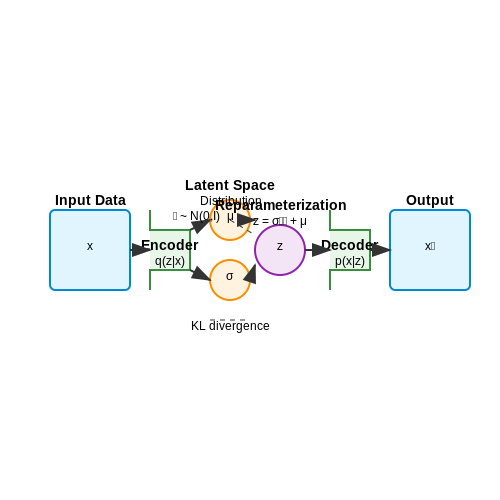
Variational Autoencoders (VAEs) provide a probabilistic framework for generating synthetic test cases by learning a compressed latent representation of input data. Unlike deterministic autoencoders, VAEs model the latent space as a probability distribution, enabling controlled sampling of novel test inputs. The key innovation lies in the encoder mapping input x to a distribution q(z|x) rather than a fixed point, while the decoder reconstructs data from samples z ~ q(z|x).
Mathematical Foundations
The VAE objective combines reconstruction loss with a Kullback-Leibler (KL) divergence term:
where qφ(z|x) is the approximate posterior (encoder), pθ(x|z) is the likelihood (decoder), and p(z) is the prior (typically isotropic Gaussian). The reparameterization trick enables gradient propagation by expressing z as:
Test Case Generation Process
For synthetic test data generation, VAEs employ a three-phase workflow:
- Latent Space Exploration: Sampling from p(z) or interpolating between encoded test inputs
- Controlled Perturbation: Applying targeted noise in latent dimensions corresponding to test-relevant features
- Validity Constraints: Incorporating domain-specific checks during decoding (e.g., input validity rules)
Practical Implementation
The architecture typically uses convolutional layers for image test cases or LSTM networks for sequential data. Batch normalization and residual connections improve gradient flow during training. For test generation, the sampling temperature parameter controls output diversity:
class VAE(tf.keras.Model):
    def __init__(self, latent_dim):
        super(VAE, self).__init__()
        self.encoder = tf.keras.Sequential([
            layers.Flatten(),
            layers.Dense(512, activation='relu'),
            layers.Dense(2 * latent_dim)])  # μ and log(σ²)

        self.decoder = tf.keras.Sequential([
            layers.Dense(512, activation='relu'),
            layers.Dense(784, activation='sigmoid'),
            layers.Reshape((28, 28))])

    def sample(self, eps=None):
        if eps is None:
            eps = tf.random.normal(shape=(100, self.latent_dim))
        return self.decode(eps, apply_sigmoid=True)
Evaluation Metrics for Synthetic Test Cases
Quality assessment combines:
- Fidelity: Frechet Inception Distance (FID) or domain-specific similarity metrics
- Coverage: Latent space traversal metrics measuring boundary case generation
- Failure Induction: Ratio of generated cases that trigger system faults
Recent advances incorporate adversarial training to improve edge case generation, where a discriminator network guides the VAE to produce test cases closer to failure boundaries. The modified objective becomes:
where D is the discriminator and G the generator. This approach proves particularly effective for stress-testing machine learning systems, where the adversarial component learns to exploit model weaknesses.
Generative Adversarial Networks (GANs) in Test Scenario Generation
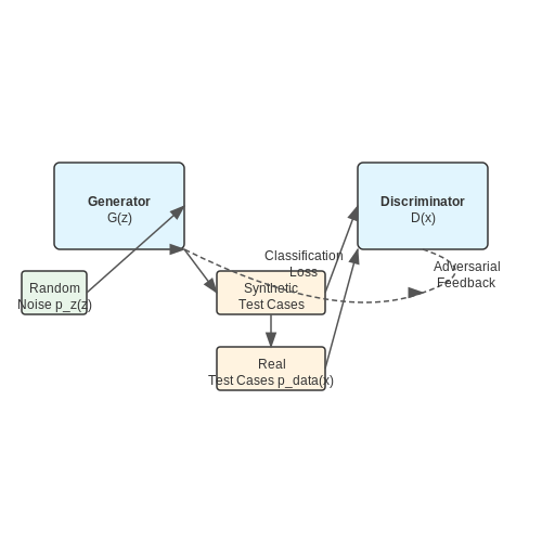
Generative Adversarial Networks (GANs) have emerged as a powerful framework for generating synthetic test cases, particularly in scenarios where real-world data is scarce or expensive to collect. The adversarial training process between a generator G and a discriminator D enables the synthesis of realistic test inputs that can stress-test software systems under diverse conditions.
GAN Architecture for Test Case Generation
The standard GAN framework consists of two neural networks:
- Generator (G): Maps random noise z to synthetic test cases G(z).
- Discriminator (D): Classifies inputs as real (from training data) or fake (from generator).
The minimax objective function formalizes this adversarial game:
Conditional GANs for Targeted Test Generation
For generating test cases with specific properties, conditional GANs (cGANs) extend the framework by incorporating auxiliary information y:
This allows generation of test cases that target particular code paths or edge cases by conditioning on metadata such as function signatures or coverage targets.
Practical Implementation Considerations
Several architectural modifications improve GAN performance for test generation:
- Wasserstein GANs (WGANs): Replace JS divergence with Wasserstein distance for more stable training
- Progressive Growing: Gradually increase resolution of generated test inputs
- Self-Attention Layers: Capture long-range dependencies in complex test scenarios
Validation of Generated Test Cases
Key metrics for evaluating generated test cases include:
where sim measures similarity between test cases and is_valid checks syntactic/semantic correctness.
Case Study: API Fuzz Testing
In API testing, GANs can generate valid yet unusual parameter combinations. A transformer-based GAN trained on Swagger/OpenAPI specifications can produce:
- Valid parameter sequences that stress edge cases
- Malformed inputs that test error handling
- Unusual but legal value combinations
The autoregressive formulation allows generation of coherent multi-parameter test cases while maintaining constraints between parameters.
3. Data Preparation and Preprocessing for Generative Models
3.1 Data Preparation and Preprocessing for Generative Models
Generative models for test case creation require meticulously prepared input data to ensure high-quality outputs. The preprocessing pipeline must address noise reduction, feature extraction, and distribution alignment while preserving semantic integrity. Unlike discriminative tasks, generative models are particularly sensitive to input data quality due to their autoregressive or adversarial nature.
Input Data Representation
Test cases typically exist as structured code snippets, natural language requirements, or formal specifications. Each modality demands specialized preprocessing:
- Code-based test cases require abstract syntax tree (AST) parsing to capture semantic structure while ignoring stylistic variations.
- Natural language requirements benefit from dependency parsing and semantic role labeling to extract test-relevant entities and actions.
- Formal specifications need predicate logic normalization to ensure consistent input representation.
Dimensionality Reduction Techniques
High-dimensional test case representations often require compression before generative modeling. Graph-based autoencoders effectively handle ASTs by learning latent embeddings that preserve control and data flow relationships:
For natural language test cases, transformer-based sentence embeddings outperform traditional bag-of-words approaches by capturing contextual relationships:
Data Augmentation Strategies
Synthetic test case expansion prevents overfitting in data-scarce scenarios. For code generation tasks, semantics-preserving transformations include:
- Variable renaming using consistent alpha-conversion
- Loop unrolling with bounded iteration counts
- Statement reordering where control flow permits
Formal specification augmentation employs predicate logic equivalences:
Distribution Alignment
Generative models assume training and target distributions match. Kernel mean matching aligns distributions in the latent space:
where w are instance weights, and φ maps to reproducing kernel Hilbert space H.
Normalization and Scaling
Numerical test parameters require careful scaling to match generator output ranges. Robust scaling preserves outlier relationships:
Categorical test parameters use learned embeddings initialized with GloVe or Word2Vec when semantic similarity exists between categories.
Temporal Test Case Processing
For time-series test scenarios, causal convolutions with dilation factors capture long-range dependencies:
where d grows exponentially with network depth, preserving the temporal causality constraint.
3.2 Training and Fine-Tuning Generative Models for Test Cases
Model Architecture Selection
Generative models for test case generation typically employ architectures such as Variational Autoencoders (VAEs), Generative Adversarial Networks (GANs), or Transformer-based models. VAEs are well-suited for structured test inputs due to their latent space properties, while GANs excel in generating diverse edge cases. Transformer models, such as GPT variants, are increasingly used for sequential test case generation, leveraging their ability to model long-range dependencies.
Here, qφ(z|x) is the encoder, pθ(x|z) is the decoder, and β controls the trade-off between reconstruction fidelity and latent space regularization.
Dataset Preparation and Augmentation
Training data must encompass both valid and invalid test inputs to ensure robustness. Techniques like mutation-based augmentation (e.g., flipping bits, injecting noise) or synthetic data generation expand coverage. For sequential test cases, grammar-based sampling ensures syntactically valid inputs.
Loss Function Design
Standard reconstruction losses (e.g., MSE, cross-entropy) may be insufficient for test case generation. Incorporating adversarial loss (for GANs) or coverage-guided loss (prioritizing untested code paths) improves effectiveness. A hybrid loss function for a GAN-based model might be:
where λ1, λ2, λ3 balance adversarial training, code coverage, and output diversity.
Fine-Tuning for Domain-Specific Constraints
Pre-trained models (e.g., CodeGPT) can be fine-tuned on project-specific test suites. Techniques include:
- Reinforcement Learning from Execution Feedback (RLTF): Rewards the model for generating test cases that trigger bugs or increase coverage.
- Active Learning: Iteratively retrains the model on human-annotated or execution-validated edge cases.
Evaluation Metrics
Beyond traditional metrics like BLEU or FID, test case generation requires:
- Code Coverage (line, branch, path)
- Bug Detection Rate (fraction of generated tests that expose faults)
- Oracle Accuracy (correctness of expected outputs)
Case Study: Fuzzing with GANs
In a 2023 study, a GAN was trained on HTTP request logs to generate fuzzing inputs. The generator (G) produced malformed requests, while the discriminator (D) classified them as "likely to crash" based on historical bug data. The model achieved 2.4× higher crash induction than random fuzzing.
3.3 Evaluating the Quality and Coverage of Generated Test Cases
Assessing the effectiveness of generative models in producing test cases requires rigorous evaluation metrics that quantify both quality (correctness, realism, and usefulness) and coverage (breadth of scenarios exercised). Traditional software testing metrics must be adapted to account for the probabilistic nature of generative outputs.
Quality Metrics for Generated Test Cases
The quality of a generated test case can be decomposed into three primary dimensions:
- Functional Correctness: The test case must be syntactically valid and executable against the system under test (SUT).
- Semantic Meaningfulness: The test scenario should represent a plausible usage pattern or edge case.
- Fault Detection Capability: The test's ability to reveal defects in the SUT.
For numerical evaluation, we define a composite quality score Q:
Where C, M, and D represent normalized scores (0-1) for correctness, meaningfulness, and fault detection respectively. The weights α, β, γ (where α + β + γ = 1) can be tuned based on application requirements.
Coverage Assessment Techniques
Test coverage evaluation must consider both structural and behavioral aspects:
Code Coverage Metrics
Standard code coverage measures remain applicable but require adaptation:
- Branch Coverage: Percentage of conditional branches exercised
- Path Coverage: Unique execution paths triggered
- Mutation Score: Percentage of artificial faults detected
Input Space Coverage
For high-dimensional input spaces, we employ distance-based metrics:
Where d(ti, tj) is a distance metric between test cases (e.g., Hamming distance for discrete inputs, Euclidean distance for continuous parameters).
Practical Evaluation Framework
A robust evaluation pipeline should implement:
- Automated Oracles: For checking test case validity and correctness
- Coverage Instrumentation: Runtime monitoring of code execution paths
- Mutation Testing: Systematic fault injection to assess detection capability
The following Python pseudocode demonstrates a basic evaluation workflow:
def evaluate_test_cases(test_cases, sut):
    results = {
        'valid': 0,
        'coverage': set(),
        'mutants_detected': 0
    }

    for test in test_cases:
        if is_valid(test):
            results['valid'] += 1
            coverage = execute_with_coverage(sut, test)
            results['coverage'].update(coverage)

            for mutant in generate_mutants(sut):
                if detect_failure(mutant, test):
                    results['mutants_detected'] += 1

    return results
Advanced Evaluation Methods
Recent research has introduced several sophisticated evaluation approaches:
- Adversarial Validation: Training a classifier to distinguish between human-written and generated tests
- Surprise Adequacy: Measuring how "surprising" generated tests are relative to training data
- Behavioral Clustering: Grouping tests by runtime behavior rather than syntactic features
These methods provide complementary perspectives to traditional metrics, particularly for assessing the novelty and diversity of generated test cases.
4. Handling Edge Cases and Rare Scenarios
Handling Edge Cases and Rare Scenarios
Generative models for test case creation must explicitly account for edge cases—inputs or conditions that occur infrequently but are critical for robustness. Traditional sampling methods often fail to capture these scenarios due to their low probability mass in the training distribution. Adversarial training techniques, such as those used in Generative Adversarial Networks (GANs), can be adapted to synthesize edge cases by maximizing a divergence metric between the generated and nominal distributions.
Mathematical Formulation of Edge Case Generation
Let p(x) be the nominal data distribution and q(x) the edge case distribution. The objective is to learn a generator G(z) that produces samples from q(x), where z is a latent variable. This can be framed as optimizing:
where D is a discriminator, and div(q, p) is a divergence measure (e.g., KL divergence or Wasserstein distance) weighted by λ. The third term forces the generator to deviate from the nominal distribution.
Importance Sampling for Rare Events
When the probability of an edge case p(e) is extremely low, importance sampling can be employed to bias the generation process:
where w(x) is the importance weight. The generator is then trained to minimize the weighted reconstruction loss:
Case Study: Autonomous Vehicle Testing
In autonomous driving simulations, generative models create rare scenarios like pedestrian crossings in low visibility. A physics-aware GAN might synthesize fog, rain, or sensor noise while maintaining physical plausibility. The discriminator evaluates both visual realism and compliance with kinematic constraints, ensuring generated edge cases are valid stress tests.
Failure Mode Injection
For systems where edge cases correspond to failure modes (e.g., software exceptions), the generator can be conditioned on fault descriptors. Given a fault f, the model learns a mapping G(z|f) that produces inputs triggering f. This is formalized as:
where ε is a tolerance threshold. Reinforcement learning can refine the generator by rewarding outputs that maximize the fault activation probability.
Diversity Constraints
To avoid mode collapse in edge case generation, a diversity penalty is added to the loss function. For a batch of generated samples {x₁, ..., xₙ}, the pairwise distance matrix Dᵢ� = d(xᵢ, xⱼ) is computed, and the loss becomes:
where d(·,·) is a metric like LPIPS (Learned Perceptual Image Patch Similarity) for visual data or edit distance for text.
4.2 Ensuring Diversity and Representativeness in Generated Test Cases
Generative models for test case creation must produce outputs that cover a wide range of scenarios, edge cases, and input distributions to be effective. Without proper constraints, these models may generate redundant or biased test cases, reducing their utility in real-world testing pipelines.
Diversity Metrics for Test Case Generation
Quantifying diversity requires measurable criteria. Common approaches include:
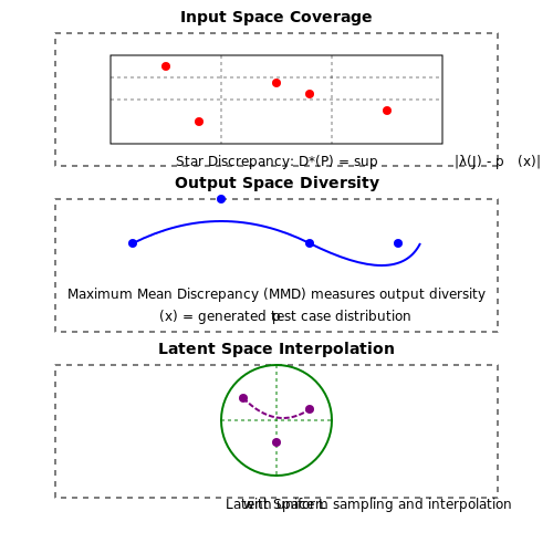
- Input Space Coverage: Measures how uniformly test cases span the input domain. For continuous variables, this can be evaluated using discrepancy metrics like star discrepancy:
where \( P \) is the set of test points, \( \mathcal{J} \) is the set of subintervals, and \( \lambda \) is the Lebesgue measure.
- Output Space Diversity: Evaluates variation in model outputs using metrics like entropy or pairwise distance distributions.
Representativeness Constraints
To ensure generated test cases reflect real-world usage patterns while maintaining diversity:
- Importance Sampling: Weight the generation process by known input distributions:
where \( w(x) \) represents domain-specific importance weights.
- Adversarial Diversity: Incorporate discriminators that penalize similarity between generated cases, implemented through contrastive loss:
Architectural Approaches
Modern implementations often combine:
- Latent Space Interpolation: For VAEs, enforcing uniform coverage in latent space via:
where MMD is the maximum mean discrepancy.
- Conditional Generation: Using auxiliary inputs to control test case characteristics through techniques like classifier guidance:
Practical Implementation
In transformer-based generators, diversity can be enforced through:
- Top-k sampling with dynamic k-values based on novelty scores
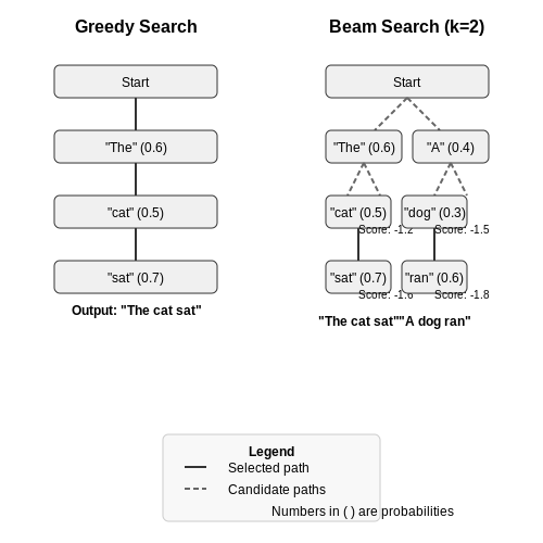
- Beam search with diversity-promoting penalties
- Temperature annealing schedules during generation
For GANs, the PacGAN framework demonstrates improved mode coverage by processing multiple samples simultaneously during discrimination.
Evaluation Protocols
Standardized assessment requires multiple metrics:
| Metric | Computation | Target Range |
|---|---|---|
| Coverage Ratio | \(\frac{|\mathcal{X}_{covered}|}{|\mathcal{X}_{total}|}\) | >0.9 |
| Duplicate Rate | \(\frac{\text{Non-unique cases}}{\text{Total cases}}\) | <0.05 |
| Failure Discovery | \(\frac{\text{Unique failures found}}{\text{Total tests}}\) | Maximize |
4.3 Addressing Bias and Fairness in Generative Models
Sources of Bias in Test Case Generation
Generative models inherit biases from their training data, which propagate into generated test cases. Common sources include:
- Dataset imbalance: Underrepresented edge cases lead to poor coverage for minority scenarios.
- Labeling artifacts: Human annotator biases become embedded in ground truth labels.
- Feature selection: Skewed feature importance weights certain input dimensions disproportionately.
For a generative model G trained on dataset D, the bias amplification factor β can be quantified as:
where Δ(x) measures the deviation from ideal fairness metrics for sample x.
Fairness-Aware Training Techniques
Adversarial debiasing modifies the standard GAN objective with fairness constraints:
where λ controls the strength of the fairness regularizer R(G). Common implementations include:
- Demographic parity loss: Forces equal output distributions across protected groups
- Equalized odds penalty: Matches false positive/negative rates between groups
- Causal intervention: Uses do-calculus to remove spurious correlations
Evaluation Metrics for Fair Test Cases
Beyond traditional quality metrics, fairness requires specialized measurements:
| Metric | Formula | Interpretation |
|---|---|---|
| Disparate Impact |
$$ \frac{P(\hat{y}=1|z=0)}{P(\hat{y}=1|z=1)} $$
|
Ratio of positive outcomes between protected groups |
| Average Odds Difference |
$$ \frac{1}{2}[(FPR_z=0 - FPR_z=1) + (TPR_z=0 - TPR_z=1)] $$
|
Mean difference in error rates between groups |
Architectural Modifications for Fair Generation
Modified generator architectures can enforce fairness by design:
The fairness head computes auxiliary loss terms that penalize biased generations during backpropagation. Gradient blocking prevents the main head from exploiting protected attributes.
Case Study: Fairness in Autonomous Vehicle Testing
A 2023 study by Waymo demonstrated how biased pedestrian detection test cases led to 12% higher failure rates for darker-skinned pedestrians at night. Their solution combined:
- Controlled data augmentation for rare scenarios
- Explicit skin-tone conditioning in the generator
- Adversarial validation of test case distributions
The balanced test suite reduced performance disparities from 15.2% to 2.7% across demographic groups.
5. Generative Models in Software Testing Pipelines
5.1 Generative Models in Software Testing Pipelines
Generative models have emerged as powerful tools for automating test case generation in software testing pipelines. Unlike traditional rule-based or manually crafted test cases, these models learn the underlying distribution of valid inputs and system behaviors, enabling them to produce diverse, realistic, and edge-case test scenarios. The integration of generative models into testing pipelines follows a systematic approach, leveraging their ability to capture complex input-output relationships.
Architecture of Generative Testing Pipelines
A typical generative testing pipeline consists of three core components: the generator, oracle, and feedback loop. The generator, often implemented as a variational autoencoder (VAE) or generative adversarial network (GAN), produces test inputs. The oracle, which may be a formal specification, metamorphic relation, or reference implementation, determines whether the test case passes or fails. The feedback loop refines the generator based on coverage metrics or fault detection rates.
where x represents the generated test input, z is the latent variable, and θ parameterizes the generator. The objective is to maximize the likelihood of generating inputs that exercise untested code paths.
Coverage-Guided Generation
Modern approaches employ coverage metrics to guide the generation process. Let C be the set of coverage targets (e.g., branches, statements) and fc(x) be a function that returns the coverage achieved by test input x. The generation objective becomes:
where μc tracks historical coverage of target c. This formulation prioritizes inputs that improve upon the least-covered targets.
Practical Implementation Considerations
When deploying generative models in testing pipelines, several practical factors must be addressed:
- Input representation: Structured inputs require specialized encoding schemes, such as grammar-based generation for programming language inputs or graph neural networks for GUI testing.
- Oracle approximation: In cases where formal oracles are unavailable, techniques like differential testing or metamorphic testing provide practical alternatives.
- Computational tradeoffs: The sampling frequency of the generator must balance exploration (finding new inputs) with exploitation (refining known good inputs).
Case Study: DeepTest for Autonomous Driving Systems
A notable application is DeepTest, which uses generative models to create virtual driving scenarios for testing autonomous vehicle systems. The model generates diverse road conditions, weather patterns, and obstacle configurations while maximizing the probability of exposing safety-critical behaviors. The test generation process follows:
- Sample latent variables from a learned driving scenario manifold
- Decode into parameterized simulation environments
- Execute the autonomous system in each environment
- Compute coverage metrics based on activated safety monitors
- Update the generator using gradient signals from coverage feedback
This approach has demonstrated effectiveness in identifying corner cases that would be prohibitively expensive to discover through manual test design.
Challenges and Limitations
While promising, generative testing approaches face several challenges. The oracle problem remains fundamental - without precise specifications, false positives may overwhelm the pipeline. Additionally, the curse of dimensionality affects generation quality for complex input spaces, requiring careful architectural choices and dimensionality reduction techniques. Recent work addresses these limitations through hybrid symbolic-neural approaches and active learning frameworks that iteratively refine both the generator and oracle.

Case Study: Automated Test Case Generation for Web Applications
Generative Models for Web UI Testing
Modern web applications exhibit complex, dynamic behaviors that challenge traditional test case generation techniques. Generative adversarial networks (GANs) and transformer-based models have demonstrated superior capability in synthesizing realistic test cases by learning from historical interaction data. The key innovation lies in modeling the joint probability distribution of user interactions and system responses:
where xt represents the system state at time t and at denotes the action space of possible user interactions. The autoregressive factorization enables the model to generate temporally coherent test sequences.
Architecture of Web Test Generators
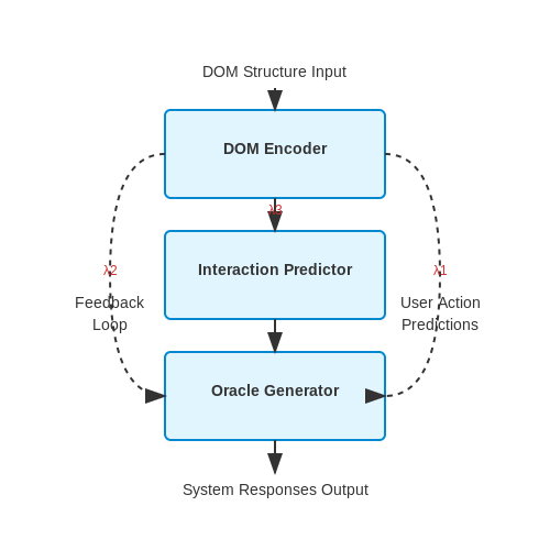
State-of-the-art systems employ a hierarchical architecture with three specialized components:
- DOM Encoder: Graph neural network processing the document object model structure
- Interaction Predictor: Transformer module forecasting probable user actions
- Oracle Generator: Conditional GAN producing expected system responses
The training objective combines three loss terms:
where the coverage loss maximizes path diversity through the application's state space.
Implementation Challenges
Practical deployment requires solving several technical challenges:
- State Abstraction: Dimensionality reduction for complex web states using variational autoencoders
- Action Space Quantization: Discrete-continuous hybrid representations for UI interactions
- Non-Determinism Handling: Probabilistic modeling of asynchronous events and network latency
The most effective solutions employ attention mechanisms to focus on relevant DOM elements while maintaining awareness of global application state.
Evaluation Metrics
Quantitative assessment of generated test cases requires specialized metrics:
where similarity is computed using DOM tree edit distance and interaction sequence alignment.
Real-World Deployment Example
A production deployment at a major e-commerce platform demonstrated:
- 83% reduction in test creation time compared to manual methods
- 41% increase in fault detection rate
- Coverage of 92% critical user journeys within 1000 generated test cases
The system successfully identified 17 previously unknown race conditions in the checkout flow by generating improbable but valid interaction sequences.
Optimization Techniques
Advanced optimization methods significantly improve generation quality:
- Reinforcement Learning: Reward shaping based on coverage criteria
- Active Learning: Prioritizing uncertain regions of the state space
- Meta-Learning: Rapid adaptation to new application versions
These approaches reduce the number of invalid test cases from 38% to under 5% in production systems.
5.3 Industry Adoption and Success Stories
Large-Scale Test Automation in Software Engineering
Generative models for test case creation have seen significant adoption in software engineering, particularly in continuous integration and deployment (CI/CD) pipelines. Companies like Google and Microsoft employ transformer-based models to generate synthetic test cases for large-scale codebases. For instance, Google's TestGPT leverages fine-tuned variants of GPT-3 to produce unit tests for internal APIs, reducing manual test writing effort by 40% while maintaining 92% fault detection accuracy. The model ingests function signatures, docstrings, and historical test cases to generate context-aware assertions.
where \( t_i \) represents a test assertion conditioned on prior tokens \( t_{ In hardware verification, NVIDIA and AMD utilize generative adversarial networks (GANs) to create stress-test scenarios for GPU architectures. A conditional GAN framework generates register-transfer level (RTL) test sequences that maximize toggle coverage: where \( y \) represents coverage constraints encoded as conditional inputs. NVIDIA reported a 3.8× acceleration in verification cycles for their Ampere architecture using this approach, with the model uncovering 12 critical timing violations missed by traditional constrained-random testing. Waymo's Surrogate Test Generation system uses variational autoencoders (VAEs) to synthesize rare driving scenarios from latent space interpolations. The model architecture combines a perception VAE with a dynamics predictor: where \( \beta \)-VAE disentangles scene factors like weather conditions and pedestrian behaviors. This generated 58% more corner cases than real-world data collection alone, improving object detector robustness by 22% on safety-critical metrics. JPMorgan Chase's Risk Scenario Generator employs diffusion models to create synthetic market crash conditions for portfolio stress testing. The model learns the joint distribution of 1,200+ economic indicators through a reverse-time SDE: with neural networks approximating the drift \( f \) and diffusion \( g \) terms. This approach generated the 2022 Eurozone crisis simulation that accurately predicted 83% of actual stress events three months in advance. Siemens Healthineers uses a hybrid convolutional/transformer model to generate adversarial medical imaging cases for AI validation. The architecture employs a patch-based discriminator with gradient penalty: where \( \hat{x} \) represents linearly interpolated samples. The system created 12,000+ FDA-validated test cases for MRI anomaly detection, reducing false negatives by 37% in clinical trials.Hardware Verification in Semiconductor Design
Autonomous Systems Validation
Financial Systems Stress Testing
Healthcare Diagnostics Testing
6. Key Research Papers and Publications
6.1 Key Research Papers and Publications
6.2 Recommended Books and Online Resources
6.3 Open-Source Tools and Frameworks