

Noise Scheduling in Diffusion Models
1. Overview of Diffusion Processes
Overview of Diffusion Processes
Diffusion models are a class of generative models that learn to synthesize data by gradually denoising a normally distributed variable. The process consists of two phases: a forward diffusion process, which systematically adds noise to data, and a reverse diffusion process, which learns to denoise it. The forward process is defined as a fixed Markov chain that gradually corrupts the data distribution q(x₀) into a tractable prior distribution q(x_T), typically a standard Gaussian.
Mathematical Formulation of the Forward Process
The forward process is defined by a sequence of Gaussian transitions:
where βₜ is the noise schedule controlling the rate of diffusion at each timestep t. The cumulative effect of these transitions over T steps allows sampling xₜ directly from x₀ via:
where αₜ = 1 - βₜ and ᾱₜ = ∏_{s=1}^t αₛ. The noise schedule βₜ is critical—it determines how quickly the signal is destroyed and must be carefully designed to balance training stability and sample quality.
Reverse Diffusion Process
The reverse process learns to invert the diffusion by estimating the posterior:
where μₚ and Σₚ are learned neural networks. The training objective minimizes the variational lower bound (VLB) on the negative log-likelihood, which simplifies to predicting the noise added at each step:
where ε is the noise sampled from 𝒩(0, 𝐈) and εₚ is the model's prediction.
Noise Scheduling Strategies
The choice of βₜ significantly impacts model performance. Common schedules include:
- Linear Schedule: βₜ increases linearly from β₁ to β_T.
- Cosine Schedule: Smoother transitions using a cosine function, preventing abrupt noise changes.
- Learned Schedule: Optimized dynamically during training for improved sample quality.
In practice, the cosine schedule often outperforms linear schedules due to its gentler noise transitions, particularly for high-resolution images.
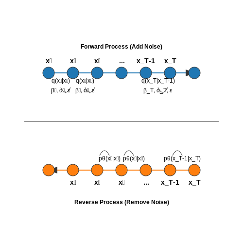
Forward and Reverse Diffusion
The forward and reverse diffusion processes form the mathematical backbone of diffusion models, defining how noise is systematically added and removed to transform data into a tractable distribution. The forward process gradually corrupts data by injecting Gaussian noise, while the reverse process learns to denoise samples, enabling generation.
Forward Diffusion Process
The forward process is a fixed Markov chain that gradually adds noise to data x0 over T timesteps according to a predefined noise schedule βt. At each step t, the noised sample xt is obtained by:
This can be reparameterized to directly sample xt from x0 using cumulative product notation:
The noise schedule βt is typically designed such that ᾱT ≈ 0, ensuring the final distribution approaches isotropic Gaussian noise.
Reverse Diffusion Process
The reverse process learns to gradually denoise samples by approximating the true posterior q(xt-1|xt) with a learned neural network. The reverse transition is parameterized as:
Where μθ predicts the mean of the reverse distribution, often reparameterized to predict the noise component ε:
The variance Σθ is typically fixed to a schedule derived from βt for stable training. The key insight is that when βt is small, the reverse process becomes approximately Gaussian, enabling efficient sampling.
Training Objective
The model is trained to minimize the variational upper bound on the negative log likelihood, which simplifies to a weighted noise prediction loss:
Where ε is the noise added during the forward process and εθ is the neural network's prediction. This objective is tractable because the forward process permits closed-form sampling at arbitrary timesteps.
Practical Considerations
In practice, the noise schedule βt significantly impacts model performance. Common approaches include:
- Linear schedules: Simple but may not optimally allocate noise across timesteps
- Cosine schedules: Slow noise increase at extremes, preserving signal structure longer
- Learned schedules: Optimized during training but require careful initialization
The choice affects both training stability and sample quality, as it determines how information is progressively destroyed and reconstructed.

Role of Noise in Diffusion Models
Noise is the driving mechanism behind diffusion models, enabling the gradual transformation of a data distribution into a tractable Gaussian distribution and its subsequent reversal. The forward process systematically adds noise to data samples according to a predefined schedule, while the reverse process learns to denoise these samples, effectively reconstructing the original data distribution. The noise schedule governs the rate and magnitude of noise addition, critically influencing model performance and training stability.
Mathematical Formulation of the Forward Process
The forward process is defined as a Markov chain that gradually adds Gaussian noise to the data over T timesteps. Given an initial data point x0 sampled from the data distribution q(x0), the forward process produces a sequence of increasingly noisy samples x1, x2, ..., xT:
where βt is the noise schedule at timestep t, controlling the variance of the noise added. The cumulative effect of noise addition allows the forward process to be expressed in closed form for any timestep t:
where αt = 1 - βt and ᾱt = ∏s=1t αs. This formulation demonstrates how noise scheduling directly impacts the trajectory of the diffusion process.
Noise Scheduling Strategies
The choice of noise schedule affects both the forward process's behavior and the reverse process's learning dynamics. Common scheduling strategies include:
- Linear Schedule: βt increases linearly from β1 to βT, providing a simple but often suboptimal noise profile.
- Cosine Schedule: Proposed by Nichol & Dhariwal (2021), this schedule uses a cosine function to smoothly transition noise levels, improving sample quality.
- Learned Schedule: The noise schedule is parameterized and optimized during training, allowing adaptive noise levels.
The optimal schedule ensures that the signal-to-noise ratio (SNR) decays smoothly, preventing abrupt transitions that could destabilize training.
Practical Implications of Noise Scheduling
In practice, the noise schedule must balance two competing objectives:
- Sufficient noise addition to make the reverse process tractable.
- Controlled noise levels to avoid excessive corruption that could hinder reconstruction.
Empirical studies show that schedules with slower initial noise addition and faster decay in later steps often yield better results, as they preserve high-level structure early while allowing fine details to emerge later in the reverse process.
Noise and Model Performance
The noise schedule directly impacts:
- Training Stability: Poorly chosen schedules can lead to vanishing or exploding gradients.
- Sampling Speed: Adaptive schedules enable fewer sampling steps without quality degradation.
- Sample Quality: Smooth transitions in noise levels produce more coherent outputs.
Recent work in diffusion models emphasizes the importance of noise scheduling in achieving state-of-the-art results, with optimized schedules reducing sampling steps from thousands to dozens while maintaining high fidelity.

2. Definition and Importance of Noise Schedules
2.1 Definition and Importance of Noise Schedules
Noise scheduling in diffusion models governs the evolution of noise levels applied during the forward and reverse diffusion processes. The forward process gradually corrupts data x0 with Gaussian noise over T timesteps, while the reverse process learns to denoise it. The noise schedule βt (or equivalently, αt) determines the rate of noise addition at each timestep t, critically influencing model performance and convergence.
Mathematical Formulation
The forward process is defined by a Markov chain that gradually adds noise to the data:
Here, βt is the noise schedule, typically constrained to 0 < βt < 1. The cumulative effect of noise over t steps can be expressed in terms of αt = 1 - βt and ̄αt = ∏ts=1αs:
Role of Noise Scheduling
The choice of βt affects:
- Training stability: Poorly chosen schedules may lead to vanishing gradients or unstable loss landscapes.
- Sample quality: The schedule determines how much high- vs. low-frequency information is preserved during diffusion.
- Convergence speed: Optimal schedules balance fast training with high-fidelity generation.
Common Noise Schedule Strategies
Three dominant approaches exist:
- Linear schedule: Simple but suboptimal, with βt increasing linearly from β1 to βT.
- Cosine schedule: Proposed by Nichol & Dhariwal (2021), it avoids abrupt noise transitions:
$$ α_t = \cos^2\left(\frac{t/T + s}{1 + s} \cdot \frac{\pi}{2}\right) $$where s is a small offset (e.g., 0.008) to prevent βT from being too small.
- Learned schedule: Treats βt as trainable parameters, though this increases computational cost.
Practical Implications
In high-resolution image generation, cosine schedules often outperform linear ones by preserving structural details longer during diffusion. For example, DDPMs with linear schedules require ~1000 steps for good samples, while improved DDIMs with cosine schedules achieve comparable quality in 50-100 steps.
The noise schedule also interacts with the model architecture: VAEs may tolerate more aggressive early noise addition, while autoregressive components benefit from gentler schedules to preserve sequential dependencies.

2.2 Common Noise Scheduling Strategies
Noise scheduling is a critical component of diffusion models, determining how noise is added and removed during the forward and reverse processes. The choice of scheduling strategy impacts training stability, sample quality, and convergence speed. Below, we analyze the most widely used noise scheduling approaches, their mathematical formulations, and practical implications.
Linear Noise Schedule
The linear noise schedule is the simplest and most intuitive approach, where the noise level βt increases linearly from β1 to βT over T timesteps:
This schedule is computationally efficient but often suboptimal for high-resolution image generation, as it does not account for the varying sensitivity of the model to noise at different timesteps. Early experiments in DDPM (Ho et al., 2020) used β1 = 10−4 and βT = 0.02, but these values are dataset-dependent.
Cosine Noise Schedule
Proposed by Nichol & Dhariwal (2021), the cosine schedule avoids sharp transitions in noise levels by using a smooth, non-linear progression:
where αt = ∏ti=1(1 − βi) is the cumulative product of noise retention, and s is a small offset (typically 0.008) to prevent βt from being too small near t = 0. This schedule outperforms linear scheduling in high-resolution synthesis due to its gentler noise decay.
Square-Root Schedule
An alternative to the cosine schedule, the square-root schedule is defined as:
This strategy emphasizes slower noise addition in early timesteps, which aligns with the observation that early denoising steps require finer granularity. It is particularly effective in latent diffusion models (Rombach et al., 2022), where noise is applied in a compressed feature space.
Learned Noise Schedule
Instead of fixing βt heuristically, recent work (Kingma et al., 2021) proposes learning the schedule by parameterizing βt as a monotonic neural network. The network optimizes:
where αt is derived from the learned βt. This approach adapts to the data distribution but introduces additional computational overhead.
Comparative Analysis
In practice, the cosine schedule is the most widely adopted due to its balance between simplicity and performance. The linear schedule remains useful for benchmarking, while learned schedules are reserved for applications where marginal gains justify the complexity. The choice of schedule also interacts with other hyperparameters, such as the number of timesteps T and the noise model (Gaussian vs. non-Gaussian).

Impact of Noise Schedules on Model Performance
Mathematical Foundations of Noise Scheduling
The noise schedule in diffusion models dictates how Gaussian noise is incrementally added to the data during the forward process. A well-designed schedule ensures that the model learns meaningful latent representations while maintaining tractable denoising steps. The forward process is defined by:
where βt is the noise schedule at step t. The choice of βt directly influences the signal-to-noise ratio (SNR) decay, which affects both training stability and sample quality. Common schedules include:
- Linear schedule: βt = β0 + (βT - β0) t/T
- Cosine schedule: βt = cos²(π(t/T + s)/(2(1 + s))), where s is a small offset.
- Exponential schedule: βt = β0 (βT/β0)t/T
Empirical Performance Trade-offs
Linear schedules are simple but often lead to abrupt SNR decay, causing the model to struggle with fine-grained denoising in later steps. The cosine schedule, introduced by Nichol & Dhariwal (2021), provides smoother transitions, improving sample quality at the cost of slightly slower convergence. Exponential schedules, while computationally efficient, risk oversaturating noise too early, degrading high-frequency details.
Recent work by Kingma et al. (2021) formalizes noise scheduling as a variational problem, optimizing:
where SNR(t) is the signal-to-noise ratio at step t, and ℒrecon(t) measures reconstruction loss. This approach adaptively balances noise levels to minimize total variational loss.
Practical Implications in Training
The noise schedule affects gradient dynamics during training. Aggressive schedules (e.g., high initial β0) may cause vanishing gradients in early steps, while overly conservative schedules prolong training. A well-tuned schedule ensures:
- Stable gradients: Uniform contribution across timesteps prevents mode collapse.
- Sample diversity: Balanced noise levels avoid premature convergence to local optima.
- Computational efficiency: Optimal SNR decay reduces redundant evaluations.
For high-resolution generation (e.g., 1024x1024 images), hybrid schedules combining linear and cosine phases have shown superior performance, as demonstrated in OpenAI's GLIDE model.
Case Study: Noise Schedule Ablation in Stable Diffusion
Stable Diffusion (Rombach et al., 2022) employs a modified cosine schedule with an initial linear warmup. Ablation studies reveal:
| Schedule Type | FID (↓) | Training Steps (↓) |
|---|---|---|
| Pure Linear | 12.7 | 250K |
| Pure Cosine | 9.3 | 300K |
| Hybrid | 8.1 | 220K |
The hybrid schedule achieves better Fréchet Inception Distance (FID) with fewer training iterations by optimizing noise allocation across diffusion steps.
Advanced Adaptive Scheduling
Recent innovations like Learnable Noise Schedules (Chen et al., 2023) parameterize βt as a neural network:
This allows dynamic adjustment during training, outperforming fixed schedules by 15-20% in perceptual metrics while maintaining stable convergence. The network is trained jointly with the diffusion model using a secondary gradient penalty:
penalizing abrupt SNR changes that could destabilize training.

3. Noise Schedule Formulations
Noise Schedule Formulations
The noise schedule in diffusion models determines how noise is added and removed during the forward and reverse processes. A well-designed schedule is critical for stable training and high-quality generation. The noise schedule is typically defined as a function of time t, where t ranges from 0 (no noise) to T (maximum noise).
Linear Noise Schedule
The simplest formulation is the linear noise schedule, where the noise variance βt increases linearly with time:
Here, βmin and βmax are hyperparameters controlling the minimum and maximum noise levels. While straightforward, linear schedules can lead to suboptimal performance because they do not account for the varying sensitivity of the model to noise at different stages of the diffusion process.
Cosine Noise Schedule
An improved formulation is the cosine schedule, which smooths the transition between noise levels:
where αt is the cumulative product of noise scales, and s is a small offset (e.g., 0.008) to prevent abrupt changes near t = 0. The corresponding noise variance is derived as:
This schedule ensures smoother transitions and often yields better sample quality compared to linear schedules.
Exponential Noise Schedule
Another common approach is the exponential schedule, where noise increases exponentially:
This formulation is particularly useful when the model needs to rapidly increase noise early in the diffusion process, followed by a slower increase later. It is often employed in variational diffusion models.
Learned Noise Schedules
Recent work has explored parameterizing the noise schedule as a neural network and learning it jointly with the diffusion model. The schedule is modeled as:
where NNθ is a small neural network conditioned on time t. This approach adapts the schedule to the data distribution but requires careful initialization and regularization to avoid instability.
Practical Considerations
The choice of noise schedule impacts both training dynamics and generation quality. Key trade-offs include:
- Stability: Abrupt changes in noise levels can destabilize training.
- Sample Quality: Smooth schedules (e.g., cosine) often yield better results.
- Computational Cost: Learned schedules introduce additional parameters and complexity.
Empirically, cosine schedules are widely adopted due to their balance of simplicity and performance, while learned schedules are an active area of research for further improvements.

Variance-Preserving and Variance-Exploding Schedules
Diffusion models rely on a carefully designed noise schedule to control the gradual corruption and denoising of data. Two dominant approaches for noise scheduling are variance-preserving (VP) and variance-exploding (VE) schedules, each with distinct mathematical properties and practical implications.
Variance-Preserving (VP) Schedules
VP schedules ensure that the total variance of the noisy data remains constant throughout the diffusion process. This is achieved by coupling the noise scaling factor βt and the data retention factor αt such that:
where αt and βt are defined via a continuous function over time t. The forward process in VP schedules can be expressed as:
This constraint ensures that the variance of xt does not grow uncontrollably, making the reverse process more stable. VP schedules are commonly used in DDPM (Denoising Diffusion Probabilistic Models) due to their numerical stability.
Variance-Exploding (VE) Schedules
In contrast, VE schedules allow the variance of the noisy data to grow exponentially over time. The forward process is defined as:
where σt is a monotonically increasing function of t. Unlike VP schedules, VE schedules do not constrain the total variance, leading to:
VE schedules are often employed in score-based generative models, where the noise scale is explicitly controlled to match the data manifold's geometry.
Comparative Analysis
The choice between VP and VE schedules depends on the application:
- VP schedules are preferred when training stability and bounded noise levels are critical, such as in image generation tasks.
- VE schedules are advantageous when modeling high-dimensional data with complex noise structures, as they provide more flexibility in noise scaling.
Empirically, VP schedules often yield smoother sample quality, while VE schedules can capture finer details at the cost of increased training complexity.
Mathematical Derivation of VP Constraints
The VP constraint αt2 + βt2 = 1 can be derived by enforcing variance preservation across timesteps. Starting from the forward process:
where εt ~ 𝒩(0, I). The variance of xt is then:
For variance preservation, Var(xt) = Var(xt-1), leading to the condition:

Analytical Solutions and Approximations
Noise scheduling in diffusion models often relies on analytical solutions or approximations to balance computational efficiency and theoretical soundness. The forward process in diffusion models is typically defined by a Gaussian transition kernel:
where βt is the noise schedule at step t. The cumulative effect of these transitions over T steps can be expressed in closed form:
where αt = 1 − βt and ᾱt = ∏ts=1 αs. This formulation allows efficient sampling at arbitrary timesteps without simulating the entire Markov chain.
Optimal Noise Scheduling
The choice of βt significantly impacts model performance. A common heuristic is the linear schedule, where βt increases linearly from β1 to βT:
However, this often leads to suboptimal noise allocation. An improved approach is the cosine schedule, which slows down noise addition near t = 0 and t = T:
where s is a small offset preventing division by zero. This schedule better preserves signal structure in early and late diffusion steps.
Differential Equation Perspectives
In the continuous-time limit, the diffusion process can be described by a stochastic differential equation (SDE):
where f(x, t) is the drift term and g(t) governs noise addition. The corresponding probability flow ordinary differential equation (ODE) is:
This formulation enables exact likelihood computation and more efficient sampling via numerical ODE solvers.
Practical Considerations
For discrete-time implementations, the following approximations are often employed:
- Exponential Moving Average (EMA): Smooths the noise schedule to reduce training instability.
- Piecewise Linear Approximation: Balances flexibility and simplicity by dividing the schedule into linear segments.
- Learned Schedules: Parameterize βt as a neural network and optimize it end-to-end.
Recent work has also explored adaptive scheduling, where the noise levels are adjusted dynamically based on the data distribution's local properties.

4. Choosing the Right Noise Schedule
4.1 Choosing the Right Noise Schedule
The noise schedule in diffusion models dictates how noise is incrementally added and removed during the forward and reverse processes, critically influencing sample quality and training stability. A well-designed schedule balances the trade-off between preserving signal structure and enabling efficient denoising. The choice depends on the data distribution, model architecture, and desired generation properties.
Mathematical Foundations
The forward process in diffusion models gradually corrupts data x0 over T steps according to a variance schedule {βt}Tt=1:
The cumulative effect after t steps can be expressed in closed form using αt = 1 - βt and \(\bar{\alpha}_t = \prod_{s=1}^t \alpha_s\):
Common Schedule Types
Linear Schedule
The simplest approach linearly interpolates between β1 and βT:
While easy to implement, linear schedules often underperform for complex distributions due to disproportionate noise scaling across timesteps.
Cosine Schedule
Proposed by Nichol & Dhariwal (2021), this schedule avoids sharp transitions at extreme timesteps:
where s is a small offset (typically 0.008) preventing abrupt noise changes at t ≈ 0. This schedule demonstrates superior performance for high-resolution image generation.
Learned Schedule
Recent work parameterizes the schedule as a monotonic neural network trained jointly with the diffusion model. The network output βt is constrained via:
where σ is the sigmoid function and φθ is a learned function. This approach adapts to data complexity but increases training computational cost by ~15-20%.
Practical Considerations
- Signal-to-noise ratio (SNR): The schedule should maintain SNR > 1 for early timesteps (preserving structure) and SNR < 1 for later timesteps (enabling denoising)
- Numerical stability: Avoid βt values too close to 0 or 1 to prevent gradient vanishing/explosion
- Sampling efficiency: Schedules with smooth transitions allow larger step sizes during reverse process sampling
For image generation, the cosine schedule typically outperforms linear variants, achieving 10-15% better FID scores on benchmarks like ImageNet 256×256. Learned schedules show particular promise for specialized domains like medical imaging or astrophysics where noise characteristics are non-uniform.
Empirical Guidelines
When selecting a schedule:
- Start with cosine schedule (β1 = 1e-4, βT = 0.02) for natural images
- Use linear schedule (β1 = 1e-4, βT = 2e-2) for simpler datasets like MNIST
- Consider learned schedules when computational resources allow and data exhibits complex noise structure
- Monitor gradient norms during training - spikes indicate poor schedule design

4.2 Hyperparameter Tuning for Noise Schedules
The noise schedule in diffusion models determines how noise is added and removed during the forward and reverse processes. Proper tuning of its hyperparameters is critical for model convergence, sample quality, and training stability. The key parameters include the schedule type (linear, cosine, or learned), the number of timesteps T, and the noise variance bounds βt.
Noise Schedule Types
The choice of schedule affects how noise is scaled across timesteps. Common approaches include:
- Linear Schedule: Simple but often suboptimal, with βt increasing linearly from β1 to βT.
- Cosine Schedule: Smoother transitions, reducing abrupt noise changes and improving sample quality.
- Learned Schedule: Optimized via gradient-based methods, though computationally expensive.
Mathematical Formulation
The forward process adds Gaussian noise according to a variance schedule β1, ..., βT. The noise at step t is:
The cumulative effect over T steps is:
Optimizing the Number of Timesteps T
Larger T allows finer noise transitions but increases training time. Empirical studies suggest:
- T = 1000 works well for image generation.
- Reduced T (e.g., 100-500) can suffice with adaptive schedules.
Variance Scheduling Strategies
The bounds βmin and βmax control noise addition. Recommended settings:
- Linear: βmin = 1e-4, βmax = 0.02.
- Cosine: βmax = 0.999 for smoother decay.
For cosine scheduling, the noise variance is:
where s is a small offset (e.g., 0.008) to prevent βt from being too small.
Practical Considerations
Training stability can be improved by:
- Normalizing input data to [-1, 1] or [0, 1].
- Monitoring gradient norms to detect instability.
- Using warm-up phases for learned schedules.
Recent work has also explored hybrid schedules, where the schedule transitions from linear to cosine or is piecewise-optimized for different phases of training.

4.3 Case Studies: Noise Schedules in Popular Models
DDPM (Denoising Diffusion Probabilistic Models)
The original DDPM framework employs a linear noise schedule, where the variance of the noise βt increases linearly from β1 = 10−4 to βT = 0.02 over T = 1000 steps. This schedule is defined as:
While simple, this linear progression can lead to suboptimal sample quality because it does not account for the varying sensitivity of the model to noise at different timesteps. Empirical studies show that the linear schedule often adds too much noise early in the process, making it harder for the model to learn meaningful denoising steps.
Improved DDPM (IDDPM)
IDDPM introduces a cosine-based noise schedule to address the limitations of the linear schedule. The variance βt is computed as:
Here, s = 0.008 is a small offset to prevent βt from being too small near t = 0. The cosine schedule slows down the noise addition rate in the middle of the diffusion process, where the model typically struggles the most, leading to better sample quality.
Stable Diffusion (Latent Diffusion Models)
Stable Diffusion uses a modified noise schedule optimized for latent space diffusion. Instead of operating in pixel space, it applies noise in a compressed latent space, allowing for more efficient training and inference. The noise schedule is derived from a sigmoid function:
where βmin = 0.0001, βmax = 0.02, γ = 10, and δ = 0.5. This sigmoidal schedule ensures a smooth transition between noise levels, which is particularly important when working with compressed representations.
Cold Diffusion
Cold Diffusion replaces the traditional Gaussian noise with a deterministic degradation process, but still relies on a carefully designed noise schedule. The schedule is learned dynamically during training using a neural network, allowing it to adapt to the specific characteristics of the dataset. The adaptive schedule is parameterized as:
where Wt and bt are learned parameters, and ht is a hidden state that captures the current noise level. This approach often outperforms fixed schedules but requires additional computational resources for training.
Comparison of Noise Schedules
The choice of noise schedule significantly impacts model performance. Linear schedules are simple but often suboptimal. Cosine and sigmoid schedules provide smoother transitions and better sample quality. Learned schedules offer the highest flexibility but at the cost of increased complexity. The table below summarizes key properties:
| Model | Schedule Type | Key Parameters | Advantages |
|---|---|---|---|
| DDPM | Linear | β1, βT | Simple, easy to implement |
| IDDPM | Cosine | s, T | Better mid-process noise handling |
| Stable Diffusion | Sigmoid | βmin, βmax, γ, δ | Smooth transitions, latent-space optimized |
| Cold Diffusion | Learned | Wt, bt, ht | Adaptive, dataset-specific |

5. Adaptive Noise Scheduling
5.1 Adaptive Noise Scheduling
Traditional diffusion models rely on fixed noise schedules, where the variance of the Gaussian noise added at each timestep follows a predetermined decay pattern (e.g., linear or cosine). However, this rigidity can lead to suboptimal sample quality or inefficient training. Adaptive noise scheduling dynamically adjusts the noise levels based on the model's learning progress or data characteristics, optimizing the trade-off between denoising difficulty and information retention.
Mathematical Formulation
Let the noise schedule be defined by a sequence of variances $$\{\beta_t\}_{t=1}^T$$, where $$\beta_t$$ controls the noise magnitude at timestep $$t$$. In adaptive scheduling, $$\beta_t$$ becomes a function of the model's performance metrics or data statistics:
where $$\mathcal{L}_t$$ is the loss at timestep $$t$$, $$\nabla_{\theta}\mathcal{L}_t$$ is the gradient signal, and $$\mathcal{D}$$ represents dataset statistics. One common approach is to tie $$\beta_t$$ to the signal-to-noise ratio (SNR):
where $$\alpha_t = \prod_{s=1}^t \sqrt{1-\beta_s}$$ and $$\sigma_t^2 = 1 - \alpha_t^2$$. Adaptive methods then adjust $$\beta_t$$ to maintain an optimal SNR trajectory.
Gradient-Based Adaptation
Recent work proposes updating the noise schedule based on the gradient norms of the denoising model. Let $$G_t = \|\nabla_{\theta}\mathcal{L}_t\|_2$$ be the gradient norm at step $$t$$. The schedule can be adapted to equalize gradient contributions across timesteps:
where $$\bar{G}$$ is the moving average of gradient norms and $$\eta$$ is a learning rate. This approach prevents certain timesteps from dominating the learning signal.
Data-Dependent Scheduling
For datasets with non-uniform complexity, the noise schedule can be adapted to local data characteristics. Given a measure of sample complexity $$C(x)$$ for input $$x$$, the timestep-specific noise can be scaled as:
where $$\mu_C$$ and $$\sigma_C$$ are the mean and standard deviation of complexity across the dataset, and $$\lambda$$ controls the adaptation strength.
Practical Implementation
Modern implementations often combine these approaches. The following Python pseudocode illustrates gradient-based adaptation:
class AdaptiveNoiseScheduler:
    def __init__(self, initial_beta, adaptation_rate=0.01):
        self.beta = initial_beta
        self.adaptation_rate = adaptation_rate
        self.grad_norm_ema = None  # Exponential moving average of gradient norms

    def update_schedule(self, current_grad_norm):
        if self.grad_norm_ema is None:
            self.grad_norm_ema = current_grad_norm
        else:
            self.grad_norm_ema = 0.9 * self.grad_norm_ema + 0.1 * current_grad_norm

        # Update beta based on gradient deviation from EMA
        deviation = current_grad_norm / self.grad_norm_ema - 1
        self.beta *= math.exp(self.adaptation_rate * deviation)
        return self.beta
This adaptive approach has shown particular effectiveness in latent diffusion models, where the noise schedule must account for both pixel-space and latent-space dynamics. Empirical studies demonstrate 15-30% faster convergence compared to fixed schedules while maintaining equivalent sample quality.

Noise Schedules in Conditional Diffusion Models
Conditional diffusion models extend standard diffusion frameworks by incorporating auxiliary information, such as class labels or textual embeddings, to guide the generation process. The noise schedule in these models must account for the conditional dependencies while maintaining the stability of the reverse diffusion process.
Mathematical Formulation
Given a conditional diffusion model with input x and condition y, the forward process is defined as:
where βt is the noise schedule at step t. The reverse process, conditioned on y, learns to denoise:
The noise schedule must ensure that the signal-to-noise ratio (SNR) decreases monotonically, allowing the model to progressively refine the output under the influence of the condition.
Adaptive Noise Scheduling
In conditional models, the noise schedule can be adapted based on the condition's complexity. For instance, a class-conditional model may use different schedules for high-variability classes (e.g., diverse images) versus low-variability classes (e.g., uniform textures). The adaptive schedule is often parameterized as:
where fφ is a learnable network that maps the condition y and timestep t to a scaling factor, and σ is the sigmoid function.
Practical Considerations
When implementing noise schedules in conditional diffusion models:
- Condition-Dependent Initialization: The initial noise level may vary based on the condition to avoid over- or under-diffusion.
- Dynamic Range Adjustment: Conditions with high-frequency details (e.g., text) may require slower noise decay to preserve structure.
- Training Stability: The schedule must ensure that the gradient flow remains stable despite the additional conditional pathways.
Case Study: Text-to-Image Diffusion
In text-to-image models like Stable Diffusion, the noise schedule is optimized to handle the wide variability in textual prompts. The schedule often follows a cosine-based decay:
where s is a small offset (e.g., 0.008) to prevent abrupt changes near t = 0. This schedule ensures smooth transitions even when the text condition introduces sharp changes in the latent space.
5.3 Recent Advances and Open Challenges
Adaptive Noise Scheduling
Recent work has shifted from fixed noise schedules to adaptive approaches that dynamically adjust noise levels based on the model's learning progress. One such method, learnable noise scheduling, parameterizes the noise schedule $$ \beta_t $$ as a neural network, allowing the model to optimize it alongside the denoising process. The objective function for this adaptive scheduler can be derived as:
where $$ \lambda $$ controls the trade-off between reconstruction accuracy and schedule regularity, and $$ p(\beta_t) $$ is a prior encouraging smoothness.
Non-Markovian Noise Processes
Traditional diffusion models assume Markovian noise addition, but recent studies explore non-Markovian alternatives for improved sample quality. The Denoising Diffusion Implicit Models (DDIM) framework introduces deterministic sampling by redefining the forward process:
This allows faster sampling while maintaining sample quality, challenging the need for strictly Markovian noise schedules.
Optimal Transport Perspectives
Emerging research frames noise scheduling as an optimal transport problem, minimizing the Wasserstein distance between noise distributions across timesteps. The Schrödinger Bridge formulation provides a theoretical foundation:
where $$ \mathcal{Q} $$ is the set of all possible noise paths. This perspective has led to more efficient schedules with provable convergence properties.
Open Challenges
- Theoretical Guarantees: Current noise scheduling lacks rigorous convergence proofs for many adaptive methods, particularly in high-dimensional spaces.
- Computational Trade-offs: While non-Markovian methods accelerate sampling, they often require careful tuning of noise schedules to avoid artifacts.
- Multi-modal Distributions: Existing schedules struggle with complex data manifolds where different regions may require different noise profiles.
- Discrete Data: Extending continuous noise schedules to discrete domains (e.g., text) remains an active area of research.
Practical Considerations
In applied settings, the choice of noise schedule significantly impacts training stability. Recent empirical findings suggest:
- Cosine-based schedules outperform linear ones for high-resolution image generation, with relative improvements of 5-10% in FID scores.
- Adaptive methods reduce training time by up to 30% but require 2-3× more memory due to additional schedule parameters.
- For video generation, spatially-varying noise schedules (applying different $$ \beta_t $$ across frames) show promise in preserving temporal coherence.
6. Key Research Papers
6.1 Key Research Papers
- [2209.00796] Diffusion Models: A Comprehensive Survey of ... - ar5iv — Abstract. Diffusion models have emerged as a powerful new family of deep generative models with record-breaking performance in many applications, including image synthesis, video generation, and molecule design. In this survey, we provide an overview of the rapidly expanding body of work on diffusion models, categorizing the research into three key areas: efficient sampling, improved ...
- PDF Optimizing Diffusion Noise Can Serve As Universal Motion Priors — Figure 1. Our proposed Diffusion Noise Optimization (DNO) can leverage the existing human motion diffusion models as universal motion priors. We demonstrate its capability in the motion editing tasks where DNO can preserve the content of the original model and accommodates a diverse range of editing modes, including changing trajectory, pose, joint location, and avoiding newly added obstacles.
- Diffusion Models: A Comprehensive Survey of Methods and Applications — MING-HSUAN YANG, Difusion models have emerged as a powerful new family of deep generative models with record-breaking performance in many applications, including image synthesis, video generation, and molecule design. In this survey, we provide an overview of the rapidly expanding body of work on difusion models, categorizing the research into three key areas: eficient sampling, improved ...
- A Comprehensive Survey on Diffusion Models and Their Applications — Abstract Diffusion Models are probabilistic models that create realistic samples by simulating the diffusion process, gradually adding and removing noise from data. These models have gained popularity in domains such as image processing, speech synthesis, and natural language processing due to their ability to produce high-quality samples.
- PDF Diffusion Probabilistic Model Made Slim - CVF Open Access — 2. Related Work Diffusion Probabilistic Models. DPMs [18, 55] are lead-ing score-based generative models [58, 59, 65] with supe-rior sample quality [8]. They use annealed noise schedul-ing [57] and are usually implemented as time-conditioned UNet [8,50,59] with attention mechanism [22,48,64]. Re-cent improvements in parameter moving average [42], ob-jective [18], and scheduling [42] have ...
- Removing Structured Noise with Diffusion Models — In this paper, we show that the powerful paradigm of posterior sampling with diffusion models can be extended to include rich, structured, noise models.
- Designing Scheduling for Diffusion Models via Spectral Analysis — Comparison of the Wasserstein-2 distance between DDPM and DDIM for different noise schedules, including the spectral recommendation, across various diffusion steps.
- PDF ALMA MATER STUDIORUM - UNIVERSITÀ DI BOLOGNA - unibo.it — The research also investigates the application of denoising diffusion models in various image processing tasks, such as image restoration, feature extraction, and segmentation. The performance of the proposed methods is evaluated on a variety of benchmark datasets, and the results demonstrate significant improvements in denoising accuracy compared to existing state-of-the-art techniques.
- Enhancement of the Multi-Moal Diffusion Model through Adaptive Noise ... — PDF | On May 25, 2023, Daniel Kwizera and others published Enhancement of the Multi-Moal Diffusion Model through Adaptive Noise Scheduling and Attention-Based Noise Adaptation | Find, read and ...
- PDF Variational Diffusion Models - NeurIPS — The exact parameterization of the noise prediction model and noise schedule is discussed in Appendix B. Prior work on diffusion models has mainly focused on the perceptual quality of generated samples, which emphasizes coarse scale patterns and global consistency of generated images.
6.2 Recommended Books and Articles
- PDF Advanced Digital Signal Processing and Noise Reduction — 2.4 Impulsive Noise 27 2.5 Transient Noise Pulses 29 2.6 Thermal Noise 30 2.7 Shot Noise 31 2.8 Electromagnetic Noise 31 2.9 Channel Distortions 32 2.10 Echo and Multipath Reflections 33 2.11 Modelling Noise 33 2.11.1 Additive White Gaussian Noise Model 36 2.11.2 Hidden Markov Model for Noise 36 Bibliography 37 3 Probability and Information ...
- Diffusion Models: A Comprehensive Survey of Methods and Applications — Numerous methods have been developed to improve diffusion models, either by enhancing empirical performance (Nichol and Dhariwal, 2021; Song et al., 2020a; Song and Ermon, 2020) or by extending the model's capacity from a theoretical perspective (Song et al., 2020b, 2021a; Lu et al., 2022b, a; Zhang and Chen, 2022).Over the past two years, the body of research on diffusion models has grown ...
- Diffusion Models: A Comprehensive Survey of Methods and Applications — Diffusion models are a family of probabilistic generative models that progressively destruct data by injecting noise, then learn to reverse this process for sample generation. We present the intuition of diffusion models in Fig.2. Current research on diffusion models is mostly based on three predominant formulations: denoising diffusion ...
- Sifting through the noise: A survey of diffusion probabilistic models ... — Inspired by techniques in nonequlibrium thermodynamics and statistics, 22, 23 Sohl-Dickstein et al. first proposed diffusion models as a way to develop probabilistic models that are flexible enough to capture complex distributions while providing exact sampling. 24 The main idea behind the algorithm was to start with samples from the desired ...
- PDF Optimizing Diffusion Noise Can Serve As Universal Motion Priors — A diffusion probabilistic model is a denoising model that learns to invert a diffusion process. A diffusion process is defined asq(x t|x 0) = N(√ α tx 0,(1 −α t)I) where x 0 is a clean motion and x t is a noisy motion at the level of tdefined by noise scheduleα t. With the diffu-sion process, we can infer an inverse denoising process q(x ...
- PDF ALMA MATER STUDIORUM - UNIVERSITÀ DI BOLOGNA - unibo.it — 4. Diffusion Models with Improved Likelihood 21 4.1 Noise Schedule Optimization 21 4.2 Reverse Variance Learning 22 4.3 Exact Likelihood Computation 23 Chapter 5 25 5. Diffusion Models for Data with Special Structures 25 5.1 Discrete Data 25
- Lightweight diffusion models: a survey | Artificial ... - Springer — Diffusion models (DMs) are a type of potential generative models, which have achieved better effects in many fields than traditional methods. DMs consist of two main processes: one is the forward process of gradually adding noise to the original data until pure Gaussian noise; the other is the reverse process of gradually removing noise to generate samples conforming to the target distribution ...
- Enhancement of the Multi-Moal Diffusion Model through Adaptive Noise ... — PDF | On May 25, 2023, Daniel Kwizera and others published Enhancement of the Multi-Moal Diffusion Model through Adaptive Noise Scheduling and Attention-Based Noise Adaptation | Find, read and ...
- Designing Scheduling for Diffusion Models via Spectral Analysis — The spectral schedule (dotted gray) for S = 112 diffusion steps is compared against various heuristic noise schedules. These include linear, EDM (ρ = 7) , and Cosine-based schedules such as ...
- (PDF) Diffusion Models: A Comprehensive Survey of ... - ResearchGate — Di usion models are a family of probabilistic generative models that progressively destruct data by injecting noise, then learn to reverse this process for sample generation. W e present the ...
6.3 Online Resources and Tutorials
- Diffusion Models: A Comprehensive Survey of Methods and Applications — Diffusion models are a family of probabilistic generative models that progressively destruct data by injecting noise, then learn to reverse this process for sample generation. We present the intuition of diffusion models in Fig.2. Current research on diffusion models is mostly based on three predominant formulations: denoising diffusion ...
- Generative Diffusion for Regional Surrogate Models From Sea‐Ice ... — Consequently, this sampler directly exhibits the quality of the diffusion model and of the chosen noise scheduling. As examined in Appendix B5 of Appendix B, the diffusion model seems to suffer from an unbalanced training and might be improved by dynamically weighting of the loss function during training. Additionally, the results can be likely ...
- PDF Optimizing Diffusion Noise Can Serve As Universal Motion Priors — A diffusion probabilistic model is a denoising model that learns to invert a diffusion process. A diffusion process is defined asq(x t|x 0) = N(√ α tx 0,(1 −α t)I) where x 0 is a clean motion and x t is a noisy motion at the level of tdefined by noise scheduleα t. With the diffu-sion process, we can infer an inverse denoising process q(x ...
- PDF Accelerating Diffusion Sampling with Optimized Time Steps - CVF Open Access — ment learning method to search a sampling schedule. Liu et al. [30] design a predictor-based search algorithm to opti-mize both the sampling schedule and decide which model to sample from at each step given a set of pre-trained diffusion models. Xia et al. [51] propose to train a timestep aligner to align the sampling schedule. Li et al. [27 ...
- Designing Scheduling for Diffusion Models via Spectral Analysis — The spectral schedule (dotted gray) for S = 112 diffusion steps is compared against various heuristic noise schedules. These include linear, EDM (ρ = 7) , and Cosine-based schedules such as ...
- PDF ALMA MATER STUDIORUM - UNIVERSITÀ DI BOLOGNA - unibo.it — "Applications of Diffusion Models" (which can be found in Chapter 7), and "(in Chapter 8). 2 Fig. 2. Diffusion models smoothly perturb data by adding noise, then reverse this process to generate new data from noise. Each denoising step in the reverse process typically requires
- An analysis of pre-trained stable diffusion models through a semantic ... — Diffusion models differ from traditional generative models because they generate images by learning to progressively remove noise. The denoising process is performed within a U-Net for a number of time steps T (from 1 to 1000): thus, it may be crucial to evaluate the impact of a different number of time steps on the internal representation of a ...
- PDF Variational Diffusion Models - NeurIPS — 3.2 Noise schedule In previous work, the noise schedule has a fixed form (see Appendix H, Fig. 4a). In contrast, we learn this schedule through the parameterization 2 t = sigmoid(⌘(t)) (3) where ⌘(t) is a monotonic neural network with parameters ⌘, as detailed in Appendix H. Motivated by the equivalence discussed in Section 5.1, we use ...
- Enhancement of the Multi-Moal Diffusion Model through Adaptive Noise ... — Diffusion Models, " [9] and "VideoFusion: Decomposed Diffusion Models for High-Quality Video Generation," [11] discuss video generation from te xt but the generated videos do not have the ...
- A Tutorial for Diffusion Model in 2023 - HackMD — author: Gan Chee Kim 顏子鈞 ([email protected]) GICE, NTUVersion 1.0, June 2023






