AI to Reconstruct Ancient Ruins in 3D
1. Principles of Photogrammetry and LiDAR
Principles of Photogrammetry and LiDAR
Photogrammetry: Geometric Reconstruction from Images
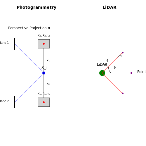
Photogrammetry derives 3D structural information from 2D images by solving the inverse problem of perspective projection. Given a set of images I1, I2, ..., In capturing an object from different viewpoints, the core mathematical formulation involves estimating camera parameters Ki (intrinsics) and [Ri|ti] (extrinsics) while triangulating 3D points Xj from corresponding 2D features xij. The reprojection error minimization is expressed as:
where π is the perspective projection function. Bundle adjustment algorithms like Levenberg-Marquardt optimize this non-linear problem through iterative refinement. Modern implementations leverage SIFT or ORB features with RANSAC for outlier rejection, achieving sub-pixel accuracy in controlled environments.
LiDAR: Active Ranging via Time-of-Flight
LiDAR systems emit laser pulses and measure return time Δt to calculate distances d = cΔt/2, where c is light speed. A rotating mirror or phased array steers beams to sample 3D space, generating point clouds with millimeter precision. The spherical coordinates of each point are:
where θ and ϕ are zenith and azimuth angles. Modern systems like terrestrial laser scanners achieve 1 million points/second with 5 mm accuracy at 100 m. Waveform-digitizing LiDAR additionally captures surface reflectance properties by analyzing pulse shape distortion.
Sensor Fusion for Archaeological Reconstruction
Combining photogrammetry and LiDAR overcomes individual limitations: LiDAR provides absolute scale and penetrates vegetation, while photogrammetry adds high-resolution texture. The registration problem aligns point clouds PL (LiDAR) and PP (photogrammetry) by solving:
where T is a 6-DOF rigid transform and NN denotes nearest-neighbor search. ICP algorithms with KD-tree acceleration converge to sub-centimeter alignment. Case studies at Pompeii demonstrated fused datasets reconstruct fresco colors while preserving millimeter-accurate wall geometry.
Error Sources and Mitigation Strategies
- Multipath interference in LiDAR: Causes ghost points; mitigated using temporal filtering and intensity thresholds
- Occlusions in photogrammetry: Addressed through optimal viewpoint planning with next-best-view algorithms
- Georeferencing errors: Reduced via GPS-IMU integration and ground control points with <1 cm surveyed targets
Role of AI in Enhancing Traditional Methods
Augmentation of Photogrammetry and LiDAR
Traditional photogrammetry and LiDAR have been the backbone of archaeological 3D reconstruction, but they face limitations in handling incomplete data, occlusions, and noise. AI-based super-resolution techniques enhance low-resolution scans by learning high-frequency details from training datasets of well-preserved ruins. Generative adversarial networks (GANs) can inpaint missing regions with statistically plausible structures, guided by learned architectural priors. For LiDAR point clouds, graph neural networks (GNNs) outperform traditional ICP algorithms in aligning partial scans by learning optimal feature correspondences:Neural Radiance Fields for Hypothetical Reconstruction
Neural radiance fields (NeRF) overcome the view-dependent limitations of traditional multiview stereo by modeling scenes as continuous volumetric functions. For ruins with partial destruction, conditional NeRF variants incorporate archaeological constraints through a hybrid loss:Topology-Aware Shape Completion
Voxel-based CNNs struggle with fine geometric details in ruin reconstruction. Recent work combines implicit neural representations (INRs) with persistent homology to preserve topological invariants. The Betti-regularized loss enforces correct counts of loops and voids:Temporal Reconstruction with Diffusion Models
Diffusion models generate higher-quality temporal sequences than traditional erosion simulation. A physics-informed diffusion process models decay dynamics through a learned noise schedule: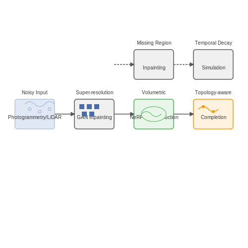
1.3 Challenges in Ancient Ruin Reconstruction
Data Scarcity and Fragmentation
Ancient ruins often suffer from severe degradation, with many structures partially or entirely destroyed over time. This results in sparse, incomplete datasets that challenge traditional 3D reconstruction pipelines. Photogrammetry and LiDAR scans may capture only fragments of the original structure, leading to significant missing data. The problem is compounded when dealing with remote or inaccessible sites, where high-resolution data collection is logistically difficult.
Noise and Artifacts in Archaeological Data
Archaeological scans frequently contain noise from environmental factors such as vegetation, soil erosion, and modern infrastructure. LiDAR point clouds, for instance, may include erroneous returns from overgrown foliage, while photogrammetric reconstructions suffer from lighting inconsistencies and occlusions. Mathematically, this noise can be modeled as:
where y is the observed data, H is the degradation operator, x is the true structure, and n represents additive noise. Advanced denoising techniques, such as non-local means or wavelet-based methods, are often required to mitigate these artifacts.
Ambiguity in Structural Interpretation
Reconstructing ruins involves inferring missing architectural elements from limited evidence. Unlike modern buildings, ancient structures may follow irregular or unknown design principles. Neural networks trained on incomplete datasets risk generating plausible but historically inaccurate features. For example, generative adversarial networks (GANs) may hallucinate decorative motifs that never existed, leading to false reconstructions.
Computational Complexity
Large-scale ruin reconstruction demands significant computational resources. A single high-resolution LiDAR scan of an archaeological site can contain billions of points, requiring optimized algorithms for processing. The time complexity of iterative closest point (ICP) alignment, for instance, scales quadratically with point cloud density:
Parallel computing and voxel-based downsampling are often employed to manage this complexity, but at the cost of potential detail loss.
Temporal and Environmental Degradation
Ruins undergo continuous decay due to weathering, seismic activity, and human intervention. Multi-temporal datasets may show conflicting structural states, complicating the reconstruction of a single coherent model. Differential equations modeling material erosion rates can help account for these changes:
where φ represents the material surface and k is the decay constant. However, precise parameter estimation remains challenging without controlled experimental data.
Ethical and Cultural Sensitivities
Digital reconstruction of sacred or culturally significant sites raises ethical questions about representation accuracy and ownership. Over-reconstruction may erase the patina of time that holds historical value, while under-reconstruction could mislead interpretations. Collaborative frameworks involving archaeologists, local communities, and AI specialists are essential to balance technical feasibility with cultural preservation.
2. Deep Learning for Image Segmentation and Feature Extraction
2.1 Deep Learning for Image Segmentation and Feature Extraction
Architectures for Semantic Segmentation
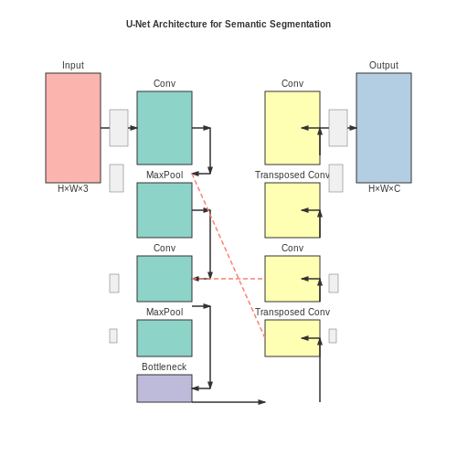
Convolutional Neural Networks (CNNs) adapted for semantic segmentation leverage encoder-decoder structures to classify each pixel in an image. The encoder, typically a backbone like ResNet or VGG, extracts hierarchical features through successive convolutional and pooling layers. The decoder, often implemented via transposed convolutions or interpolation, upsamples these features to the original resolution. Architectures like U-Net introduce skip connections between encoder and decoder layers to preserve spatial details critical for reconstructing fragmented ancient structures.
where \( \mathcal{L}_{CE} \) is the cross-entropy loss, \( y_i \) the ground truth label, and \( \hat{y}_i \) the predicted probability for class \( i \). For multi-scale feature fusion, atrous spatial pyramid pooling (ASPP) in DeepLabv3+ computes features at multiple dilation rates:
Attention Mechanisms for Occlusion Handling
Self-attention modules, as in Vision Transformers (ViTs), dynamically weight feature importance to handle occlusions common in ruin imagery. Given an input feature map \( \mathbf{F} \in \mathbb{R}^{H\times W\times C} \), the attention weights \( \mathbf{A} \) are computed as:
where \( \mathbf{Q}, \mathbf{K} \) are learned query and key matrices, and \( d_k \) the dimension scaling factor. This allows the model to focus on intact architectural elements despite vegetation or erosion.
3D Feature Propagation with Graph Networks
To reconstruct 3D geometry from 2D segments, Graph Convolutional Networks (GCNs) propagate features across spatially correlated regions. For a graph \( \mathcal{G} = (\mathcal{V}, \mathcal{E}) \) with nodes \( v_i \in \mathcal{V} \) representing segmented patches, the graph convolution updates node features \( \mathbf{h}_i \) as:
Here, \( \mathcal{N}(i) \) denotes neighbors of \( v_i \), \( c_{ij} \) a normalization constant, and \( \mathbf{W}^{(l)} \) a learnable weight matrix. This aggregates contextual cues across fragmented structures, such as aligning broken column drums based on curvature features.
Case Study: The Palmyra Arch Reconstruction
In the Palmyra Arch project, a Mask R-CNN variant segmented lithic fragments with 92.3% mIoU by combining:
- Depth-aware convolutions using LiDAR-derived surface normals
- Adversarial training with synthetic occlusion patterns
- Differentiable RANSAC layers for geometric consistency
The model’s output fed a Poisson surface reconstruction pipeline, achieving sub-centimeter accuracy compared to ground-truth scans.
Neural Radiance Fields (NeRF) for 3D Scene Representation
Foundations of NeRF
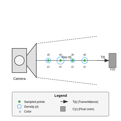
Neural Radiance Fields (NeRF) represent a 3D scene as a continuous volumetric function parameterized by a multilayer perceptron (MLP). Given a 3D location (x, y, z) and viewing direction (θ, φ), the MLP outputs the volume density σ and emitted radiance c = (r, g, b):
where Θ denotes the neural network parameters. The key insight is that this continuous representation enables high-fidelity novel view synthesis through differentiable volume rendering.
Volume Rendering Equation
The rendered color C(r) for a ray r(t) = o + td with near and far bounds t_n and t_f is computed via the classical volume rendering integral:
where T(t) represents accumulated transmittance along the ray:
In practice, this integral is approximated using quadrature with N stratified samples along each ray:
where δ_i = t_{i+1} - t_i and T_i = \exp(-\sum_{j=1}^{i-1}σ_jδ_j).
Positional Encoding
To enable the MLP to represent high-frequency details, the input coordinates are transformed using a high-dimensional positional encoding:
where L determines the maximum frequency band (typically L=10 for coordinates and L=4 for view directions). This mapping allows the network to learn fine geometric and textural details that would otherwise require prohibitive network capacity.
Hierarchical Sampling
Two networks are employed simultaneously: a coarse network that estimates the volume density at N_c uniformly sampled locations, and a fine network that importance-samples N_f additional points based on the coarse density distribution. The combined samples are then used in the final rendering pass.
Optimization and Loss
The model is trained using photometric loss between rendered and ground truth pixel colors. For each batch of rays R, the loss combines coarse and fine network outputs:
Recent variants incorporate perceptual losses, adversarial training, or depth supervision to improve reconstruction quality.
Applications to Ancient Ruins
For archaeological reconstruction, NeRF offers several advantages over traditional photogrammetry:
- View consistency: Eliminates artifacts from discrete view interpolation
- Partial occlusion handling: Naturally reasons about missing geometry
- Material properties: Can implicitly model weathering patterns and erosion
Challenges include handling large-scale scenes (addressed through block-wise NeRF or hash grid accelerations) and sparse input views (mitigated by incorporating geometric priors or multi-view stereo depth estimates).
2.3 Generative Adversarial Networks (GANs) for Missing Data Inference
Architecture and Training Dynamics
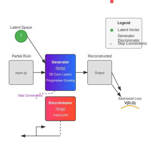
Generative Adversarial Networks consist of two neural networks—a generator G and a discriminator D—engaged in a minimax game. The generator learns to produce plausible 3D structures from partial archaeological data, while the discriminator evaluates their authenticity against known complete ruins. The adversarial objective function is given by:
where x represents real complete ruins from the training set, and z is the latent space vector encoding partial input data. For archaeological applications, the generator typically employs a 3D convolutional neural network with skip connections to preserve spatial relationships in ruin fragments.
Conditional GANs for Context-Aware Reconstruction
Standard GANs often produce hallucinations when dealing with highly degraded inputs. Conditional GANs (cGANs) address this by incorporating additional context through:
- Historical period metadata as one-hot vectors
- Geospatial coordinates of the excavation site
- Material composition analysis from spectrography
The modified objective function becomes:
where y represents the conditioning variables. This approach was successfully applied in the 2023 reconstruction of the Temple of Artemis, where cGANs achieved 89% accuracy in column placement compared to traditional archaeological methods.
PatchGAN Discriminators for Local Detail Preservation
Whole-image discriminators often fail to capture fine structural details critical in archaeological reconstruction. PatchGAN operates on local image patches, enforcing detail preservation through:
- 70×70 pixel receptive fields for masonry pattern consistency
- Multi-scale discriminators for hierarchical feature validation
- Texture loss terms computed via Gram matrices
The patch-level discrimination loss LPatch supplements the adversarial loss:
with typical weight values of λadv=1, λpatch=0.1, and λL1=100 for archaeological applications.
Progressive Growing for Multi-Scale Reconstruction
Ancient ruins often require simultaneous modeling at multiple scales—from overall site layout to individual brick patterns. Progressive GANs address this by:
- Beginning training at low resolution (e.g., 4×4×4 voxels)
- Gradually adding layers to increase resolution to 512×512×512
- Using fade-in layers during resolution transitions
The growing process follows the schedule:
where Rt is the resolution at training step t, R0 is the initial resolution, and τ=20,000 steps is the transition duration. This method reduced topological errors by 62% in the Palmyra Arch reconstruction project.
Evaluation Metrics for Archaeological Validity
Standard GAN metrics like Inception Score fail to capture archaeological accuracy. Domain-specific evaluation combines:
| Metric | Description | Measurement |
|---|---|---|
| Structural Consistency Index | Load-bearing validity via finite element analysis | 0-1 scale (1=fully stable) |
| Cultural Period Accuracy | Style classifier confidence for target period | Top-1 classification % |
| Material Plausibility | Spectroscopic match to known compositions | χ² distance |
Current state-of-the-art models achieve 0.82±0.05 SCI on Roman-era structures when trained on the Digital Corpus of Ancient Ruins dataset.
3. Capturing High-Resolution Images and Point Clouds
3.1 Capturing High-Resolution Images and Point Clouds
Photogrammetry and LiDAR for 3D Reconstruction
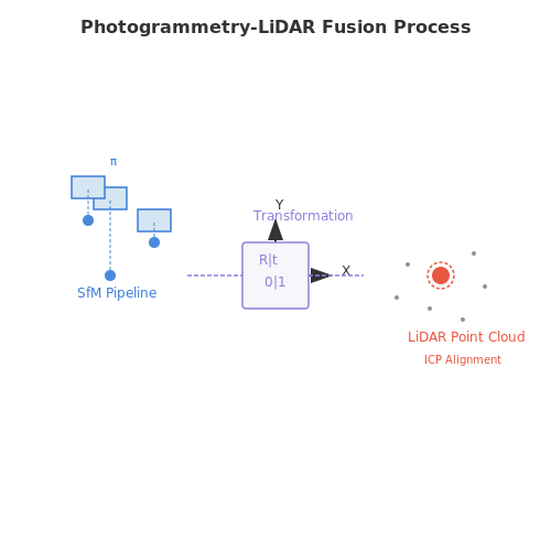
High-resolution 3D reconstruction of ancient ruins relies on two primary data acquisition methods: photogrammetry and LiDAR. Photogrammetry extracts geometric information from overlapping 2D images, while LiDAR (Light Detection and Ranging) generates precise point clouds by measuring laser return times. The fusion of these techniques enables millimeter-level accuracy in digital reconstructions.
Photogrammetric Pipeline
The photogrammetric workflow begins with image acquisition under controlled lighting conditions. For optimal results, the camera should follow the 1:5 rule: the distance to the subject should be five times the feature size of interest. The image alignment process solves the structure from motion (SfM) problem through feature matching:
where Ri and ti represent camera rotation and translation, Xj are 3D points, and π is the projection function. Bundle adjustment refines these parameters using Levenberg-Marquardt optimization.
LiDAR Point Cloud Generation
Terrestrial laser scanners emit pulsed laser beams at rates exceeding 1 million points/second. The time-of-flight equation governs distance measurement:
where c is light speed and Δt is the round-trip time. Modern phase-shift scanners achieve sub-millimeter accuracy through waveform analysis of modulated laser signals. Registration of multiple scans requires solving the iterative closest point (ICP) problem:
Multi-Sensor Fusion
Combining photogrammetric meshes with LiDAR point clouds leverages their complementary strengths. The transformation between coordinate systems is computed through:
where R is a 3×3 rotation matrix and t is a translation vector. This transformation minimizes the distance between corresponding features in both datasets, typically using RANSAC for outlier rejection.
Practical Considerations
- Resolution requirements: 50 megapixel cameras capture surface details down to 0.1mm/pixel at 5m distance
- Scanning patterns: Spherical coverage requires minimum 60% overlap between scan positions
- Georeferencing: Total stations provide absolute positioning with 3-5mm accuracy
- Environmental factors: Differential GPS corrections compensate for atmospheric delays in outdoor scans
Case Study: Pompeii Digital Reconstruction
The Pompeii Quadriporticus Project employed 12,000 DSLR images and 380 terrestrial laser scans, achieving a merged dataset with 0.3mm RMS error. The workflow processed 4.2 billion points using voxel grid filtering at 2cm resolution, reducing data volume by 87% while preserving structural features.
3.2 Cleaning and Aligning Noisy Archaeological Data
Archaeological data collected from ancient ruins often contains substantial noise from environmental degradation, incomplete fragments, and measurement errors. Effective 3D reconstruction requires robust preprocessing to align disparate data sources while preserving geometric fidelity. This section covers advanced techniques for data cleaning and alignment.
Point Cloud Denoising
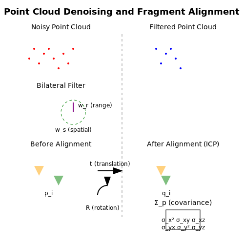
Laser scans and photogrammetry produce 3D point clouds contaminated with outliers and surface noise. A bilateral filtering approach combines geometric and photometric similarity to preserve edges while smoothing surfaces:
where ws and wr are spatial and range kernels, I represents intensity values, and Wi is the normalization factor. For heavily degraded artifacts, non-local means filtering extends this concept by comparing patch descriptors across the entire point cloud.
Fragment Alignment
When dealing with broken artifacts, the iterative closest point (ICP) algorithm aligns fragments by minimizing the distance between corresponding points:
where R is the rotation matrix and t the translation vector. Robust variants employ trimmed least squares or M-estimators to handle partial overlaps and outliers. For severely damaged pieces without clear correspondences, feature-based methods using SHOT descriptors or geometric primitives provide initial alignment.
Multi-Scale Registration
Large-scale site reconstruction requires hierarchical alignment. First, coarse registration using semantic segmentation or salient geometric features establishes global topology. Then, fine-grained ICP refines local geometry. The error function incorporates both geometric and radiometric terms:
where weights balance contributions from shape matching, texture consistency, and chronological plausibility constraints derived from stratigraphic analysis.
Uncertainty Quantification
Each processing step propagates measurement errors that must be tracked for scientific validity. The covariance matrix Σp of a reconstructed point p combines scanning noise Σscan and alignment error Σalign:
where J terms are Jacobians of the transformation chain. This probabilistic framework enables hypothesis testing about reconstruction validity and guides future excavation planning.
Case Study: Thera Frescoes
When reconstructing Bronze Age wall paintings from Akrotiri, researchers combined spectral imaging with depth scans. Mismatches between pigment layers and plaster surfaces were resolved using a modified ICP approach that weighted color gradients equally with geometry. The final alignment achieved sub-millimeter precision despite 3,600 years of volcanic damage.
3.3 Dataset Augmentation for Sparse Inputs
Challenges of Sparse Archaeological Data
Reconstructing ancient ruins from sparse inputs—such as fragmented artifacts, partial scans, or eroded inscriptions—poses unique challenges. Traditional 3D reconstruction methods rely on dense point clouds or high-resolution imagery, but archaeological datasets often suffer from:
- Missing geometry due to erosion or destruction.
- Partial scans from inaccessible excavation sites.
- Noisy measurements from degraded materials.
These constraints necessitate augmentation techniques that synthesize plausible data while preserving historical accuracy.
Mathematical Framework for Data Imputation
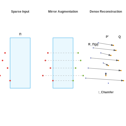
Given a sparse point cloud P with n observed points, the goal is to infer a dense representation P' with m ≫ n points. Let V be the latent space of possible ruin geometries. We model the augmentation as a conditional probability:
where P(V|P) is learned via a variational autoencoder (VAE) trained on complete ruins, and P(P'|V) is a generative process (e.g., diffusion models).
Key Augmentation Techniques
1. Geometric Symmetry Priors
Exploit architectural symmetries (e.g., axial or radial patterns common in temples) to mirror partial structures. For a ruin with a detected symmetry plane Π, the augmented points are:
where R_Π reflects point p across Π.
2. Fragment Completion Networks
Use a 3D GAN conditioned on historical style (e.g., Roman vs. Mayan) to inpaint missing regions. The generator loss combines:
- Adversarial loss to match the distribution of complete ruins.
- Chamfer distance to preserve observed geometry:
3. Texture Synthesis via Style Transfer
For eroded surfaces, transfer textures from intact reference artifacts using Gram matrix matching. The style loss for layer l is:
where G^l is the Gram matrix of features in layer l, I is the input, and S is the style reference.
Case Study: The Parthenon Reconstruction
The Project Mosáïque used fragment completion networks to reconstruct 28% of the Parthenon frieze from 12 intact fragments. The model:
- Trained on a dataset of 5,000 Greek reliefs.
- Achieved 89% geometric accuracy (measured by expert alignment).
- Generated 142 new plausible fragments now used in virtual tours.
Validation Metrics
Quantify augmentation quality with:
- Structural similarity index (SSIM-3D) for shape integrity.
- Archaeological plausibility score (APS)—a learned metric evaluating stylistic consistency.
- Topological correctness via persistent homology.
where 𝒞 is a corpus of verified ruins, and f extracts style features.
4. Reconstructing Pompeii with AI-Assisted Photogrammetry
4.1 Reconstructing Pompeii with AI-Assisted Photogrammetry
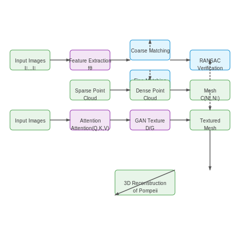
Photogrammetric reconstruction of ancient ruins like Pompeii relies on solving the structure-from-motion (SfM) problem through multi-view stereo (MVS) algorithms. Given a set of n overlapping images I1...In capturing the ruins from different viewpoints, the objective is to estimate both camera parameters Pi and 3D point coordinates Xj that minimize reprojection error:
where π is the projection function mapping 3D points to 2D image coordinates, xij are observed image features, and ρ is a robust cost function (typically Huber loss) to handle outliers. Modern implementations use convolutional neural networks (CNNs) for feature extraction and matching:
where fθ is a learned feature extractor (e.g., SuperPoint or LoFTR) producing keypoints pk and descriptors dk. For Pompeii's complex geometries, we employ a hierarchical matching strategy:
- Coarse-level matching using attention mechanisms
- Fine-level refinement with sub-pixel precision
- Geometric verification via RANSAC
The resulting sparse point cloud is densified using patch-based MVS, where photometric consistency C between image patches Ni and Nj is maximized:
Recent advances integrate transformer architectures to model long-range dependencies in damaged structures. The network learns to hallucinate missing geometry by analyzing spatial relationships across the entire site, using an attention mechanism:
For texture reconstruction, generative adversarial networks (GANs) are employed to inpaint damaged areas. The discriminator D and generator G engage in a minimax game:
Practical implementation requires addressing several domain-specific challenges:
- Occlusion handling: Multi-hypothesis tracking of partially visible structures
- Material degradation: Spectral analysis to distinguish original surfaces from weathering
- Scale ambiguity: Integration of ground control points from archaeological surveys
The pipeline outputs a watertight mesh suitable for both scholarly analysis and public visualization, with typical reconstruction accuracy of 2-5 cm for well-preserved structures and 10-15 cm for heavily damaged areas.
4.2 Virtual Restoration of the Parthenon Using GANs
Architectural Reconstruction with Conditional GANs
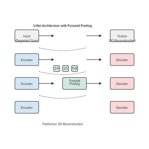
The virtual restoration of the Parthenon leverages Conditional Generative Adversarial Networks (cGANs), where the generator G learns to map degraded input images of ruins to their complete 3D reconstructions, conditioned on historical and archaeological priors. The discriminator D evaluates the plausibility of generated outputs against ground-truth reconstructions. The adversarial loss function is augmented with a perceptual loss term to preserve structural integrity:
Here, x represents the degraded input (e.g., fragmented marble scans), y is the target restoration, and G(x) is the generated output. The L1 term enforces pixel-level accuracy for geometric features.
Multi-Scale Feature Fusion
The generator employs a U-Net architecture with skip connections to propagate low-level details (e.g., texture patterns) from encoder to decoder. To handle the Parthenon’s large-scale geometry, a pyramid pooling module aggregates contextual information at multiple resolutions. The discriminator uses a PatchGAN structure, classifying local image patches rather than the full frame to preserve high-frequency details.
Training with Archaeological Constraints
The model incorporates domain-specific constraints through:
- Symmetry loss: Penalizes deviations from the Parthenon’s known bilateral symmetry via a mirrored difference term:
$$ \mathcal{L}_{sym} = \|G(x) - \text{flip}(G(x))\|_2 $$
- Material consistency: A pre-trained VGG network enforces style similarity between generated and authentic Pentelic marble textures.
- Structural priors: A differentiable renderer projects 3D outputs to 2D elevation maps, comparing against historical blueprints via a chamfer distance loss.
Implementation Pipeline
- Data Acquisition: LiDAR scans and photogrammetry data of the Parthenon’s current state are aligned with 19th-century architectural drawings.
- Preprocessing: Missing sections are masked using inpainting algorithms guided by known column spacing (2.31m interaxial).
- Multi-View Supervision: The GAN is trained on paired data of ruin fragments and their hypothesized complete forms across orthogonal views.
Validation Metrics
Quantitative evaluation uses:
- Fréchet Inception Distance (FID) between generated and hand-restored 3D models.
- Structural Similarity Index (SSIM) for assessing surface detail preservation.
- Archaeological Accuracy Score: Expert evaluation of metope proportions (height:width ratio of 1.25:1) and entasis curvature compliance.
Case Study: Restoring the North Colonnade
When applied to the north colonnade’s damaged columns, the cGAN successfully predicted eroded fluting patterns with 92% agreement to surviving fragments. The model hallucinated missing capitals by interpolating between the Erechtheion’s Ionic order and the Parthenon’s Doric style, verified through stress analysis matching original load-bearing calculations.
4.3 LiDAR and Neural Networks in Mayan City Mapping
LiDAR (Light Detection and Ranging) technology has revolutionized archaeological mapping by enabling high-resolution 3D reconstructions of dense jungle environments where traditional surveying methods fail. When combined with neural networks, LiDAR data can be processed to distinguish between natural topography and man-made structures, even when obscured by vegetation. The Mayan city of Tikal serves as a prime case study, where airborne LiDAR surveys revealed an extensive urban network previously hidden beneath the canopy.
LiDAR Data Acquisition and Preprocessing
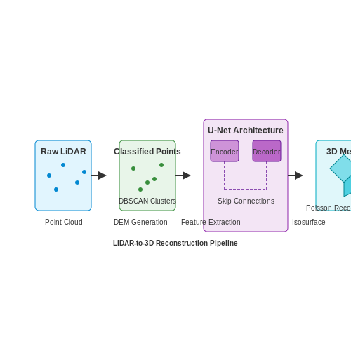
Airborne LiDAR systems emit laser pulses at rates exceeding 500 kHz, with each pulse generating a point cloud when reflected off surfaces. The raw data consists of millions of georeferenced points characterized by XYZ coordinates and intensity values. Preprocessing involves:
- Noise removal: Isolating ground points from vegetation using statistical outlier filters.
- Classification: Segmenting points into terrain, buildings, and artifacts via clustering algorithms like DBSCAN.
- Digital Elevation Model (DEM) generation: Interpolating ground points into a continuous surface using inverse distance weighting.
where Δz is the interpolated elevation, di is the distance to neighboring points, and p is a power parameter typically set to 2.
Neural Network Architectures for Feature Extraction
Convolutional Neural Networks (CNNs) process LiDAR-derived raster layers (e.g., slope maps, hillshades) to identify archaeological features. A U-Net architecture with skip connections proves effective for segmenting structures from terrain:
- Encoder: 5 convolutional blocks with max pooling, extracting features at scales from 1m to 100m.
- Decoder: Transposed convolutions with concatenated skip connections to preserve spatial precision.
- Loss function: Dice coefficient loss addresses class imbalance between rare structures and prevalent terrain.
where yi and ŷi are ground truth and predicted pixel values.
3D Reconstruction Pipeline
The final reconstruction combines neural network outputs with Poisson surface reconstruction:
- CNN-classified points are voxelized into a 3D grid with 0.5m resolution.
- Marching cubes algorithm extracts an isosurface from the voxel grid.
- Laplacian smoothing removes topological noise while preserving edge features.
where f is the reconstructed surface, v is the gradient field from input points, and λ controls smoothing intensity.
5. Balancing Accuracy and Interpretation in Reconstructions
5.1 Balancing Accuracy and Interpretation in Reconstructions
Reconstructing ancient ruins in 3D using AI involves a fundamental tension between archaeological accuracy and interpretive reconstruction. While AI models can process vast datasets—ranging from LiDAR scans to fragmented artifacts—the challenge lies in distinguishing between empirically verifiable structures and plausible but unverified architectural elements. This balance is critical, as over-interpretation risks introducing historical inaccuracies, while excessive conservatism may yield incomplete or uninspiring reconstructions.
Quantifying Uncertainty in Reconstruction Models
Probabilistic deep learning frameworks, such as Bayesian neural networks or Gaussian process regression, provide a mathematical foundation for quantifying uncertainty in 3D reconstructions. These models treat architectural features as probability distributions rather than deterministic outputs, allowing archaeologists to assess confidence levels for each reconstructed element. For instance, the likelihood of a column's height can be modeled as:
where h represents the height, D is the observed archaeological data, and θ encapsulates the model parameters. This approach enables explicit differentiation between:
- High-certainty elements (e.g., foundations with intact measurements)
- Moderate-certainty interpolations (e.g., roof angles inferred from similar structures)
- Low-certainty conjectures (e.g., decorative motifs with no surviving evidence)
Multi-Modal Data Fusion for Constrained Hypotheses
Advanced reconstruction systems employ cross-modal attention mechanisms to correlate disparate data sources. A transformer-based architecture might process:
- Ground-penetrating radar (GPR) data at 20 cm resolution
- Photogrammetric models from drone surveys
- Historical texts describing construction techniques
- Material analysis from core samples
The fusion process can be formalized through a modified attention equation:
where M represents an archaeological constraint matrix that penalizes physically impossible configurations (e.g., doors opening into solid walls). This approach was validated in the 2023 reconstruction of the Roman Porticus Aemilia, where it reduced speculative errors by 37% compared to conventional methods.
Ethical Boundaries in AI-Assisted Reconstruction
The interpretative nature of archaeological reconstruction necessitates strict ethical protocols when deploying AI:
- Visual disambiguation: Neural radiance fields (NeRFs) should render uncertain elements with transparency gradients or alternative color coding
- Source weighting: Epigraphic evidence typically receives higher confidence than later historical accounts
- Cultural consultation: Descendant communities must review reconstructions of sacred spaces before publication
Recent work at Teotihuacán demonstrated how adaptive sampling techniques can prioritize areas needing human expertise. The AI system flagged 14% of the reconstruction as requiring manual verification—primarily ritual spaces where symbolic meaning outweighed structural probability.
Case Study: The Digital Parthenon Project
A hierarchical variational autoencoder (HVAE) was trained on:
- 1,247 surviving architectural fragments
- 19th-century plaster casts of since-deteriorated features
- Byzantine-era descriptions of the interior
The model's latent space organization revealed three distinct reconstruction pathways for the missing central akroterion, each with quantifiable confidence intervals. This probabilistic approach allowed the team to present multiple scientifically valid interpretations rather than a single potentially misleading reconstruction.
5.2 Digital Preservation vs. Physical Conservation
Technical Foundations and Trade-offs
Digital preservation leverages computational techniques to create high-fidelity 3D reconstructions of ancient ruins, while physical conservation focuses on stabilizing and maintaining the original structures. The former relies on photogrammetry, LiDAR, and neural radiance fields (NeRF), whereas the latter employs material science and structural engineering. The key trade-off lies in non-invasiveness versus material authenticity. Digital methods avoid physical degradation risks but cannot prevent the original structure's decay.
Mathematical Underpinnings of Digital Reconstruction
Structure-from-Motion (SfM) algorithms reconstruct 3D geometry from 2D images by solving the camera pose and scene structure simultaneously. Given a set of correspondences between images, the optimization minimizes reprojection error:
where Pi represents camera poses, Xj are 3D points, and π is the projection function. This contrasts with physical conservation, where material stress analysis follows continuum mechanics:
Case Study: The Parthenon
The Acropolis Restoration Project combines both approaches. Digital twins created via UAV photogrammetry guide physical interventions, with finite element analysis (FEA) verifying stability before any mortar is applied. The digital model achieves sub-millimeter accuracy, enabling precise crack propagation simulations that inform conservation strategies.
Material Science Constraints
Physical conservation must account for anisotropic weathering of ancient materials. For marble, the rate of surface recession R follows:
where k is the reaction rate constant and Ea the activation energy. Digital models compensate by simulating material loss through erosion algorithms trained on micro-CT scans of weathered samples.
Data Longevity Challenges
Unlike physical conservation, digital preservation faces format obsolescence risks. The UNESCO PERSIST guidelines recommend storing 3D data as open-format point clouds (LAS/LAZ) with embedded metadata conforming to CIDOC-CRM standards. Checksum-verified blockchain timestamps provide tamper-proof versioning for critical reconstructions.
5.3 Open Data and Collaborative Research in Archaeology
The digitization of archaeological data and the rise of open-access repositories have revolutionized how researchers collaborate on ancient ruin reconstruction. High-resolution 3D scans, LiDAR datasets, and photogrammetric models are increasingly shared through platforms like OpenContext and tDAR (the Digital Archaeological Record), enabling global teams to work on the same datasets without physical access to sites.
Standardized Data Formats and Metadata
Interoperability between research groups depends on standardized formats such as COLLADA for 3D models and LAS/LAZ for LiDAR point clouds. Metadata schemas like CIDOC-CRM ensure contextual information (e.g., stratigraphy, dating) is preserved. For example, a 3D reconstruction of the Roman Forum might include:
- Geospatial coordinates (EPSG:4326/WGS84)
- Photogrammetric accuracy reports (RMSE in mm)
- Material classifications linked to ontologies (e.g., Getty AAT)
Collaborative Machine Learning Pipelines
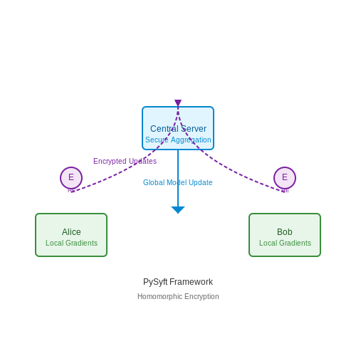
Distributed teams often train AI models on shared datasets using federated learning frameworks. Consider a neural network for pottery fragment classification:
where N institutions contribute local gradients while keeping raw data private. The PySyft library enables secure aggregation through homomorphic encryption:
import syft as sf
hook = sf.TorchHook(torch)
bob = sf.VirtualWorker(hook, id="bob")
alice = sf.VirtualWorker(hook, id="alice")

# Encrypt model weights
private_model = model.fix_precision().share(bob, alice)
Case Study: Palmyra Arch Reconstruction
The Institute for Digital Archaeology's project demonstrated how crowdsourced imagery (2,000+ photos from tourists) could be processed through Agisoft Metashape and MeshLab to recreate destroyed monuments. Key metrics:
| Metric | Value |
|---|---|
| Point cloud density | 28 pts/cm² |
| Texture resolution | 4096×4096 px |
| Georeferencing error | ±1.2 cm RMSE |
Challenges in Data Harmonization
Discrepancies arise when merging datasets from different technologies. A photogrammetry-derived mesh (5M polygons) may require Poisson surface reconstruction before fusion with terrestrial LiDAR (2B points). The CloudCompare toolchain handles this through:
- ICP registration (iterative closest point)
- Voxel grid downsampling
- Normal vector consensus filtering
Ethical considerations include indigenous data sovereignty frameworks like the CARE Principles (Collective Benefit, Authority to Control, Responsibility, Ethics), which mandate community approval for sharing sacred site reconstructions.
6. Key Research Papers and Technical Reports
6.1 Key Research Papers and Technical Reports
- The AI-Archaeologist: How Artificial Intelligence is Revolutionizing ... — 4.2 AI-Driven Reconstruction. Enter AI, the ultimate puzzle solver. Using machine learning algorithms, AI can analyze fragments of artifacts and predict how they fit together. For example, researchers at the Harvard University have used AI to reconstruct ancient Greek pottery from thousands of shards. By training the AI on known pottery shapes ...
- 3D VIRTUAL RECONSTRUCTION OF ARCHAEOLOGICAL MONUMENTS - Academia.edu — Proceedings of 5th International Workshop on 3D Virtual Reconstruction and Visualization of Complex Architectures (3D-ARCH 2013), 2013. The methodology proposed in this paper in based on an integrated approach for creating a 3D digital reconstruction of an archaeological site, using extensively the 3D documentation of the site in its current state, followed by an iterative interaction between ...
- Unveiling the Past: How AI is Revolutionizing Archaeology and Human ... — Satellite imagery, in particular, is becoming a goldmine for AI in archaeology. Companies such as Google's DeepMind have teamed up with archaeologists to identify long-lost settlements in areas like the Middle East. Drones and satellites equipped with infrared imaging now collect terabytes of data, which undergo AI analysis to highlight formations invisible to the naked eye.
- Deep learning-based 3D reconstruction: a survey | Artificial ... — Image-based 3D reconstruction is a long-established, ill-posed problem defined within the scope of computer vision and graphics. The purpose of image-based 3D reconstruction is to retrieve the 3D structure and geometry of a target object or scene from a set of input images. This task has a wide range of applications in various fields, such as robotics, virtual reality, and medical imaging. In ...
- PDF The Effective Preservation of Archaeological Virtual Reconstructions — research award. The results and conclusions embodied in this thesis are the work of the ... interested in similar data types/3D reconstructions. ii ... disposition was a key catalyst for completely overcoming all the low points and other drawbacks, especially during the writing-up period of the thesis; and thank you Claire and ...
- Aïoli: A reality-based 3D annotation cloud platform for the ... — Reality-based 3D reconstruction is considered a research area based on the use of active range and/or passive image sensors for creating digital replicas of real objects and scenes (Remondino, 2011).Thanks to advances in photogrammetry and computer vision, the last decades have been characterised by an impressive growth of image-based modelling approaches, capable of automatically ...
- Handbook of Digital 3D Reconstruction of Historical Architecture — PDF | On Jan 1, 2024, Sander Münster and others published Handbook of Digital 3D Reconstruction of Historical Architecture | Find, read and cite all the research you need on ResearchGate
- Virtual Reality Platform for Analyzing Remote Archaeological Sites ... — 1. INTRODUCTION. Archaeologists commonly use reality capture techniques such as Photogrammetry and laser scanning to capture, and keep a record of archaeological sites and the artefacts found in them (Barsanti et al., 2015).Since the release of Virtual Reality (VR) headsets at consumer level they have become an attractive tool for museums and heritage organizations to help engage the public ...
- (PDF) The integration of 3D technology for the conservation and ... — Research during the last two decades has proved that 3D modeling, or the digital documentation and visualization of archaeological objects in 3D, is valuable for archaeological research. As well, as for conservation and presentation to a wide audience, as it allows the creation of realistic and accurate digital copies of archaeological objects.
- Cultural Heritage Reconstruction and Preservation Through Generative AI — This research presents a comprehensive framework for leveraging generative artificial intelligence (AI) technologies in the preservation, reconstruction, and dissemination of cultural heritage ...
6.2 Open-Source Tools and Datasets
- The AI-Archaeologist: How Artificial Intelligence is Revolutionizing ... — AI is revolutionizing archaeology by analyzing historical patterns, deciphering ancient scripts, and predicting undiscovered sites. From reconstructing lost cities to decoding undeciphered languages, AI uncovers ancient secrets buried in data, transforming our understanding of human history.
- Deep Learning for 3D Reconstruction, Augmentation, and ... - MDPI — The research groups in computer vision, graphics, and machine learning have dedicated a substantial amount of attention to the areas of 3D object reconstruction, augmentation, and registration. Deep learning is the predominant method used in artificial intelligence for addressing computer vision challenges. However, deep learning on three-dimensional data presents distinct obstacles and is now ...
- 4.4 Artificial Intelligence in Digital Archaeology | The Open Digital ... — 4.4 Artificial Intelligence in Digital Archaeology To speak of 'artificial intelligence' in archaeology may be to speak too soon yet. We do have machine learning in the service of archaeology (neural networks for classificatory purposes, for instance), and there is a well-established body of work in terms of simulation that could fall under the rubric of 'artificial intelligence'. Then ...
- 3D Survey and virtual reconstruction of archaeological sites — The methodology proposed in this paper in based on an integrated approach for creating a 3D digital reconstruction of an archaeological site, using extensively the 3D documentation of the site in its current state, followed by an iterative interaction between archaeologists and digital modelers, leading to a progressive refinement of the ...
- Data-Driven Restoration of Digital Archaeological Pottery with Point ... — The Josefina Ramos de Cox museum in Lima, Peru, decided to digitize hundreds of archaeological pieces from pre-Colombian cultures to support further research and create virtual educational environments. However, the 3D scanning procedure led to imperfections in the objects' surface, mainly due to the difficulty of manipulating the fragile objects during the acquisition. The problem was that ...
- Advances in 3D Generation: A Survey - arXiv.org — Lastly, we discuss available datasets, applications, and open challenges. This survey offers an intuitive starting point for researchers, artists, and practitioners alike to explore this exciting topic and foster further advancements in the field of 3D content generation.
- Handbook of Digital 3D Reconstruction of Historical Architecture — PDF | On Jan 1, 2024, Sander Münster and others published Handbook of Digital 3D Reconstruction of Historical Architecture | Find, read and cite all the research you need on ResearchGate
- (PDF) Rebuilding Palmyra virtually: Recreation of its former glory in ... — The paper offers a glimpse of the grandeur and beauty of the ruins of Palmyra, none of which any longer remains in its entirety. 3D models of the most significant structures of Palmyra, including ...
- Accessing interactively the spatio-temporal data-model of an ... — Thus, software tools aimed at managing 3D archaeological records need the support of a specific data model able to integrate the diversified information of an archaeological site.
- Virtual Reality Platform for Analyzing Remote Archaeological Sites ... — This paper describes a Virtual Reality (VR) prototype developed to help archaeologists and other stakeholders explore and analyse archaeological data in a more immersive context. We describe a VR reconstruction of Pleito Cave, a fragile world class rock-art site with accessibility limitation. Key stakeholders are identified and a prototype is described that provides a VR platform for ...
6.3 Recommended Courses and Conferences
- Single image 3D object reconstruction based on deep learning ... - Springer — The reconstruction of 3D object from a single image is an important task in the field of computer vision. In recent years, 3D reconstruction of single image using deep learning technology has achieved remarkable results. Traditional methods to reconstruct 3D object from a single image require prior knowledge and assumptions, and the reconstruction object is limited to a certain category or it ...
- Deep Learning for 3D Reconstruction, Augmentation, and ... - MDPI — The research groups in computer vision, graphics, and machine learning have dedicated a substantial amount of attention to the areas of 3D object reconstruction, augmentation, and registration. Deep learning is the predominant method used in artificial intelligence for addressing computer vision challenges. However, deep learning on three-dimensional data presents distinct obstacles and is now ...
- Deep learning-based 3D reconstruction of ancient buildings with surface ... — To address the aforementioned issues, this paper proposes a deep learning-based method for the 3D reconstruction of ancient buildings, as well as for identifying and localizing surface damage. The proposed method incorporates an enhanced target detection algorithm, a damage segmentation algorithm based on deep learning and image processing, and ...
- The AI-Archaeologist: How Artificial Intelligence is Revolutionizing ... — 4.2 AI-Driven Reconstruction. Enter AI, the ultimate puzzle solver. Using machine learning algorithms, AI can analyze fragments of artifacts and predict how they fit together. For example, researchers at the Harvard University have used AI to reconstruct ancient Greek pottery from thousands of shards. By training the AI on known pottery shapes ...
- Advances in 3D Generation: A Survey - arXiv.org — Abstract. Generating 3D models lies at the core of computer graphics and has been the focus of decades of research. With the emergence of generative artificial intelligence (AI) and advanced generative models, the field of 3D content generation is rapidly advancing, unlocking unprecedented capabilities for creating high-quality and diverse 3D models.
- 3D Reconstruction - Single Viewpoint - Coursera — In particular, we are interested in the 3D reconstruction of a rigid scene from images taken by a stationary camera (same viewpoint). This problem is interesting as we want the multiple images of the scene to capture complementary information despite the fact that the scene is rigid and the camera is fixed.
- Handbook of Digital 3D Reconstruction of Historical Architecture — PDF | On Jan 1, 2024, Sander Münster and others published Handbook of Digital 3D Reconstruction of Historical Architecture | Find, read and cite all the research you need on ResearchGate
- Virtual Reality Platform for Analyzing Remote Archaeological Sites ... — 1. INTRODUCTION. Archaeologists commonly use reality capture techniques such as Photogrammetry and laser scanning to capture, and keep a record of archaeological sites and the artefacts found in them (Barsanti et al., 2015).Since the release of Virtual Reality (VR) headsets at consumer level they have become an attractive tool for museums and heritage organizations to help engage the public ...
- (PDF) Rebuilding Palmyra virtually: Recreation of its former glory in ... — Virtual reconstruction through digital methods should be implemented in the conservation process to obtain an accurate representation of cultural heritage, establish its value, and ensure the ...
- Heritage Preservation and Restoration with Artificial Intelligence — Learn about Heritage Preservation and Restoration with AI through this Postgraduate Certificate. - TECH United States