Classifier-Free Guidance in Diffusion Models
1. Overview of Diffusion Processes
1.1 Overview of Diffusion Processes
Diffusion processes describe the stochastic evolution of a system over time, where particles or states undergo random displacements due to thermal or noise-driven fluctuations. Mathematically, these processes are modeled using stochastic differential equations (SDEs) or partial differential equations (PDEs), depending on whether a microscopic or macroscopic perspective is adopted.
Mathematical Foundations
The canonical form of a diffusion process is given by the Itô stochastic differential equation:
Here, Xt represents the state at time t, μ is the drift term governing deterministic evolution, σ is the diffusion coefficient controlling noise intensity, and dWt is a Wiener process increment (Gaussian noise). The Fokker-Planck equation provides an equivalent deterministic description of the probability density p(x, t):
Connection to Score-Based Models
In modern generative modeling, diffusion processes are reversed to transform noise into structured data. The key insight is that the score function ∇x log p(x) can be estimated via neural networks, enabling iterative denoising. For a Gaussian diffusion process with variance schedule β(t), the forward process is:
This admits a closed-form marginal distribution at any timestep:
where αt = 1-βt and ᾱt = Πs=1tαs.
Practical Considerations
Several design choices critically impact diffusion model performance:
- Noise schedule: The βt schedule determines how quickly information is destroyed. Common choices include linear, cosine, and learned schedules.
- Discretization steps: While the continuous-time formulation is elegant, practical implementations require careful discretization balancing computational cost and approximation error.
- Architecture: U-Nets with residual connections and attention mechanisms are standard for score estimation, though recent work explores transformer-based architectures.
Historical Context
The theoretical foundations trace back to Einstein's 1905 work on Brownian motion, while the machine learning adaptation builds on Langevin dynamics and annealed importance sampling. The modern deep learning incarnation was catalyzed by Sohl-Dickstein et al.'s 2015 formulation and later popularized by DDPM and score-based approaches.
Visualization
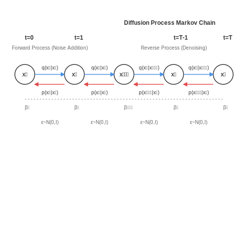
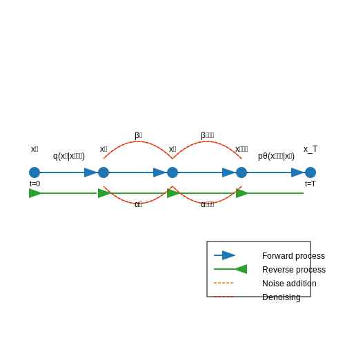
A typical diffusion process can be visualized as a gradual corruption of data through additive noise, followed by a learned reversal. The forward process transforms a sharp data distribution into an isotropic Gaussian, while the reverse process reconstructs the data manifold through iterative refinement.

Forward and Reverse Diffusion
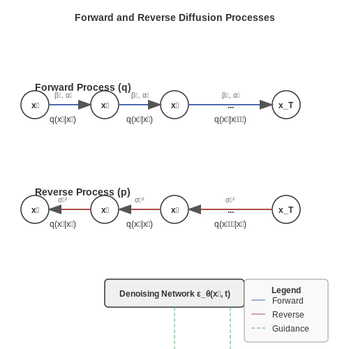
Diffusion models operate through two fundamental processes: forward diffusion, which gradually corrupts data by adding noise, and reverse diffusion, which learns to denoise and reconstruct the original data. These processes are mathematically grounded in stochastic differential equations (SDEs) and their discretized counterparts.
Forward Diffusion Process
The forward process transforms a data sample x₀ from the real data distribution q(x) into a sequence of increasingly noisy samples x₁, x₂, ..., x_T by iteratively applying Gaussian noise. This is modeled as a Markov chain with fixed variance schedules β_t:
For continuous-time analysis, the forward process can be described by a stochastic differential equation (SDE):
where f(x,t) is the drift coefficient, g(t) is the diffusion coefficient, and w is a Wiener process. The variance-preserving SDE commonly used in diffusion models has:
Reverse Diffusion Process
The reverse process learns to invert the forward diffusion by estimating the score function ∇_x log q(x_t). This is achieved through a neural network ε_θ that predicts the noise component:
where the mean μ_θ is parameterized as:
and α_t = 1-β_t, \bar{α}_t = ∏_{s=1}^t α_s. The reverse SDE corresponding to the forward process is given by:
where \bar{w} is a reverse-time Wiener process. This formulation enables sampling through numerical SDE solvers or probability flow ODEs.
Practical Implementation Considerations
In practice, the noise prediction network ε_θ is trained using a weighted L2 loss:
where t is uniformly sampled from [1,T], x_0 ∼ q(x_0), and ε ∼ \mathcal{N}(0,I). The weighting scheme affects sample quality, with common choices being:
- Uniform weighting: λ(t) = 1
- SNR weighting: λ(t) = \bar{α}_t/(1-\bar{α}_t)
- Truncated weighting: λ(t) = \sqrt{\bar{α}_t/(1-\bar{α}_t)}
The choice of noise schedule β_t significantly impacts both training dynamics and sample quality. Common schedules include linear, cosine, and learned schedules, with the cosine schedule often providing better performance:
Training Objectives for Diffusion Models
The training objective for diffusion models revolves around learning a sequence of denoising steps that gradually transform a simple noise distribution into a complex data distribution. The core idea is to define a forward process that systematically corrupts data with Gaussian noise and then train a neural network to reverse this process.
Forward Process and Noise Scheduling
The forward process is defined as a fixed Markov chain that gradually adds Gaussian noise to the data according to a predefined schedule. Given a data point x0 sampled from the true data distribution q(x0), the forward process produces a sequence x1, ..., xT by:
where βt is the noise schedule controlling the rate of corruption at each step. The cumulative effect of this process allows sampling xt directly from x0:
where αt = 1 - βt and ᾱt = ∏s=1t αs.
Reverse Process and Denoising Objective
The reverse process learns to gradually denoise the data by estimating q(xt-1|xt) using a neural network. The model is trained to predict the noise component ε added at each step, minimizing the following objective:
where εθ is the neural network predicting the noise, and t is uniformly sampled from {1, ..., T}. This simplified loss is derived from the variational lower bound (VLB) of the log-likelihood, focusing on the most significant term for high-quality sample generation.
Practical Considerations
In practice, the noise schedule βt is critical for stable training. Common choices include linear, cosine, or learned schedules that balance fast inference with high-quality generation. Additionally, techniques like variance-preserving transformations ensure numerical stability:
This formulation maintains consistent signal-to-noise ratios across diffusion steps, improving training convergence.
Classifier-Free Guidance
When conditioning on class labels or text prompts, classifier-free guidance modifies the training objective to jointly learn conditional and unconditional denoising paths. The model is trained with randomly dropped conditioning (e.g., 10-20% of the time), enabling flexible control during inference via:
where w is the guidance scale, trading off sample diversity for fidelity to the condition c.
2. Role of Classifiers in Guided Diffusion
Role of Classifiers in Guided Diffusion
In guided diffusion models, classifiers play a crucial role in steering the denoising process toward samples that satisfy specific conditions, such as class labels or semantic attributes. The core idea is to leverage gradients from a pre-trained classifier to bias the sampling trajectory toward regions of the data distribution that align with the desired condition. This approach, introduced in Classifier Guidance, modifies the unconditional score estimate $$ \nabla_{\mathbf{x}_t} \log p(\mathbf{x}_t) $$ by incorporating classifier gradients.
Mathematical Formulation
The guided score function combines the unconditional score with the gradient of the classifier's log-probability $$ \nabla_{\mathbf{x}_t} \log p(y|\mathbf{x}_t) $$, scaled by a guidance weight w:
Here, w controls the trade-off between sample quality and condition adherence. Higher w sharpens alignment with the condition but may reduce diversity. The classifier gradient term acts as a directional bias, pushing samples toward regions where the classifier assigns high probability to the target class y.
Practical Challenges
Classifier guidance introduces two key challenges:
- Classifier Training: The classifier must be trained on noisy data $$ \mathbf{x}_t $$ to provide meaningful gradients at all timesteps. This requires joint training or fine-tuning on progressively noised inputs.
- Gradient Scale: Classifier gradients can dominate the unconditional score, leading to adversarial artifacts. Adaptive scaling or gradient clipping is often necessary.
Architectural Implications
Effective classifier guidance typically employs a noise-conditional classifier, where the classifier architecture mirrors the diffusion model's time-embedding structure. For example:
where $$ f_\phi $$ shares the U-Net backbone of the diffusion model but replaces the final layer with a classification head. This design ensures temporal consistency in gradient signals.
Empirical Observations
In practice, classifier guidance exhibits several emergent properties:
- Sample-Classifier Feedback: The denoising process can exploit classifier blind spots, requiring robust classifiers with Lipschitz-constrained gradients.
- Annealed Guidance: Progressive reduction of w during sampling often improves results, analogous to temperature scheduling in annealing methods.
The computational overhead of classifier guidance stems primarily from backpropagation through the classifier at each sampling step. This motivates the development of classifier-free alternatives, which we explore in subsequent sections.
2.2 Limitations of Classifier-Based Guidance
Classifier-based guidance in diffusion models relies on an auxiliary classifier to steer the sampling process toward desired outputs. While effective, this approach introduces several critical limitations that hinder scalability, robustness, and practical deployment.
Dependency on Auxiliary Classifiers
The method requires training a separate classifier on noisy data, which must be compatible with the diffusion process. This classifier must be trained at every noise level t, leading to significant computational overhead. The gradient of the classifier's log-likelihood, ∇x log pφ(y|xt, t), is used to guide the denoising process:
where s is the guidance scale and σt is the noise schedule. Training such a classifier is non-trivial, especially for high-dimensional data, as it must generalize across all noise levels.
Adversarial Sensitivity
Classifier-based guidance is susceptible to adversarial perturbations. Small changes in xt can lead to large shifts in the classifier's gradient, destabilizing the sampling process. This sensitivity arises because the classifier is trained on noisy inputs, where small perturbations can disproportionately affect decision boundaries.
Limited Applicability to Unconditional Generation
The method inherently requires labeled data for classifier training, making it unsuitable for unconditional generation tasks. Even when labels are available, the classifier may fail to capture complex, multi-modal distributions, leading to mode collapse or biased sampling.
Error Accumulation in Sampling
Errors in the classifier's gradient estimates compound over the sampling trajectory. Since each step depends on the previous one, inaccuracies propagate, potentially driving the sample away from the true data manifold. This issue is exacerbated at high guidance scales (s ≫ 1), where over-reliance on the classifier can distort outputs.
Computational and Memory Overhead
Maintaining and querying the classifier at every denoising step doubles the computational cost compared to unconditional sampling. For large-scale models like Stable Diffusion, this overhead becomes prohibitive, limiting real-time applications.
Case Study: Text-to-Image Generation
In text-conditioned diffusion models, classifier-based guidance was initially used to align generated images with text prompts. However, the need for a separate text-conditional noise predictor introduced bottlenecks. For instance, early versions of GLIDE required a 3.5B-parameter classifier, making inference impractical for consumer hardware.
Introduction to Classifier-Free Guidance
Classifier-free guidance (CFG) is a technique in diffusion models that enables conditional generation without relying on an auxiliary classifier. Unlike classifier-guided diffusion, which requires training a separate model to estimate gradients for conditioning, CFG integrates conditioning directly into the diffusion process by jointly training a conditional and unconditional model.
Mathematical Formulation
The core idea of CFG involves interpolating between conditional and unconditional score estimates. Let εθ(xt, y, t) be the noise prediction network conditioned on input y, and εθ(xt, t) be its unconditional counterpart. The guided prediction is computed as:
where w is the guidance scale controlling the strength of conditioning. This can be rewritten as:
Training Procedure
During training, the model learns both conditional and unconditional denoising simultaneously by randomly dropping the conditioning signal y with some probability pdrop. This is implemented by replacing y with a null token ∅ during forward passes:
The null token ∅ is typically implemented as a zero vector or learned embedding. Common values for pdrop range from 0.1 to 0.2, striking a balance between conditional quality and unconditional generation capability.
Practical Advantages
CFG offers several benefits over classifier guidance:
- Simplified training: Eliminates the need to train and maintain a separate classifier network
- Improved stability: Avoids potential issues with classifier gradient estimation at high noise levels
- Flexible control: The guidance scale w can be adjusted at inference time without retraining
- Better sample quality: Empirical results show CFG often produces more coherent samples than classifier guidance at equivalent guidance strengths
Implementation Considerations
When implementing CFG, several practical aspects must be considered:
- The choice of guidance scale w significantly impacts output quality. Values between 7-15 often work well, with higher values producing more conditional but potentially less diverse samples
- The null token implementation affects model behavior. Learned embeddings often outperform zero vectors but require additional parameters
- The dropout probability pdrop influences the trade-off between conditional and unconditional performance. Too high values may degrade conditional generation quality
Empirical Results
Experiments on ImageNet 256×256 generation show CFG achieves comparable FID scores to classifier guidance while being more computationally efficient. The technique has become standard in modern diffusion architectures like Stable Diffusion, where it enables precise control over text-to-image generation without requiring separate classifier models.
3. Mathematical Formulation of Classifier-Free Guidance
3.1 Mathematical Formulation of Classifier-Free Guidance
Classifier-free guidance modifies the standard diffusion process by combining conditional and unconditional score estimates without relying on an external classifier. The key idea is to train a single model that can operate in both conditional and unconditional modes, then interpolate between these modes during sampling.
Score Estimation in Diffusion Models
In diffusion models, the forward process gradually adds noise to data x₀ over T steps according to a variance schedule βₜ:
The reverse process learns to denoise by estimating the score function ∇ₓ log pₜ(xₜ|y), where y is an optional conditioning input. The model ε₀(xₜ, t, y) is typically trained to predict the noise added at each step.
Classifier Guidance vs. Classifier-Free Guidance
Traditional classifier guidance uses Bayes' rule to decompose the score:
Classifier-free guidance avoids the need for a separate classifier p(y|xₜ) by training a single model that can estimate both conditional and unconditional scores. The model is trained with y randomly dropped (typically with probability 10-20%) to enable unconditional generation.
Interpolation of Conditional and Unconditional Scores
The guided score estimate ε̂₀ is computed as:
where w is the guidance scale and ∅ represents the unconditional case. This can be rewritten as:
When w = 1, we recover standard conditional generation. Higher values of w (typically 5-15) increase adherence to the conditioning signal at the potential cost of sample diversity.
Practical Implementation
The implementation requires:
- A conditional diffusion model trained with random null conditioning
- Modified sampling that computes both conditional and unconditional predictions
- Proper scaling of the guidance weight w to balance fidelity and diversity
The gradient of the combined score estimate becomes:
This formulation shows that classifier-free guidance effectively amplifies the difference between conditional and unconditional score estimates, similar to how classifier guidance amplifies the classifier gradient.
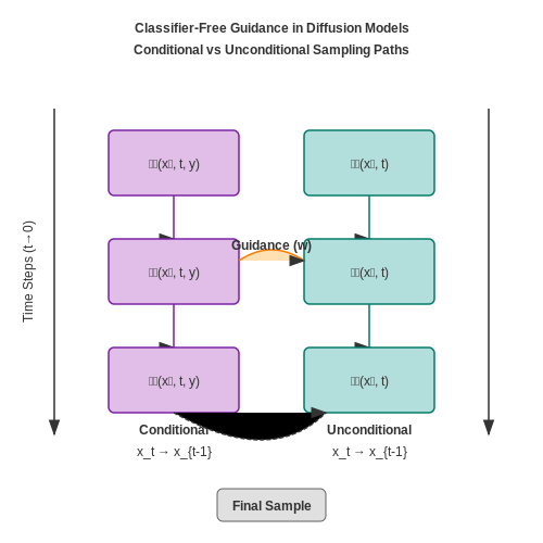
Conditional vs. Unconditional Sampling
Diffusion models generate samples by progressively denoising a random initial state, guided either by unconditional priors or conditional inputs. The distinction between these two modes lies in how the score function—the gradient of the log-likelihood—is estimated during the reverse diffusion process.
Unconditional Sampling
In unconditional sampling, the model learns the data distribution p(x) without external guidance. The score function ∇ₓ log p(x) is approximated directly by a neural network ϵₚ(xₜ, t), trained to predict noise at each timestep t. The reverse process iteratively refines the sample using:
where αₜ and σₜ are noise scheduling parameters, and z is random noise.
Conditional Sampling
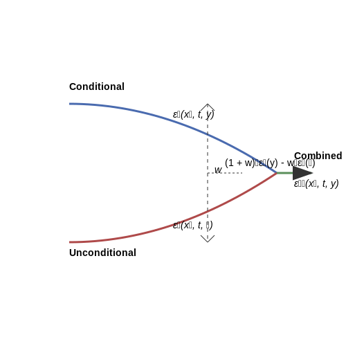
Conditional sampling introduces an auxiliary input y (e.g., class labels or text embeddings) to steer generation. The score function becomes ∇ₓ log p(x|y), implemented via a conditional network ϵₚ(xₜ, t, y). Classifier-free guidance avoids explicit classifiers by interpolating between conditional and unconditional scores:
Here, w controls guidance strength. When w = 0, the model reduces to unconditional sampling; higher w amplifies the influence of y.
Trade-offs and Practical Considerations
- Sample Quality vs. Diversity: Conditional sampling often improves fidelity at the cost of reduced diversity, as the model adheres to y.
- Training Complexity: Classifier-free guidance requires joint training of conditional and unconditional models, increasing compute overhead.
- Guidance Scale: Excessive w can lead to adversarial artifacts, while insufficient w yields weak conditioning.
In practice, the choice between conditional and unconditional sampling depends on the application—e.g., text-to-image synthesis favors strong conditioning, while artistic generation may prioritize diversity.
3.3 Practical Implementation in Diffusion Models
Classifier-free guidance modifies the standard diffusion process by combining conditional and unconditional score estimates without relying on an auxiliary classifier. The core idea is to train a single model that can operate in both conditional and unconditional modes, enabling flexible control over sample quality and diversity.
Architecture Modifications
The implementation requires a conditional diffusion model where the conditioning signal y can be explicitly dropped during training. This is achieved by randomly setting y to a null value (e.g., zero vector or special token) with some fixed probability puncond (typically 0.1 to 0.2). The model learns to estimate both ∇x log p(x|y) and ∇x log p(x) through this dropout mechanism.
Sampling with Guidance
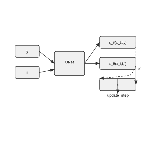
During sampling, the conditional and unconditional score estimates are combined linearly with a guidance scale w:
where w > 1 increases the influence of the conditional signal. This can be interpreted as moving away from low-likelihood regions while preserving sample diversity.
Gradient Computation
The effective gradient during sampling decomposes into two components:
This formulation avoids the instability issues of classifier-based guidance while maintaining precise control over sample characteristics. The directional component pushes samples toward regions where the conditional density exceeds the unconditional density.
Implementation Considerations
- Null embedding design: The null embedding should be distinct from valid conditioning signals but lie in the same embedding space.
- Guidance scale tuning: Typical values range from 2-10, with higher values producing more conditional samples at the cost of diversity.
- Training stability: The unconditional dropout probability must be carefully balanced to maintain good conditional modeling performance.
Pseudocode Implementation
def guided_sample(model, x_t, t, y, w=7.5):
    # Get conditional and unconditional predictions
    eps_cond = model(x_t, t, y)
    eps_uncond = model(x_t, t, null_embedding)

    # Combine with guidance scale
    eps = eps_uncond + w * (eps_cond - eps_uncond)

    # Apply diffusion update
    x_{t-1} = update_step(x_t, eps, t)
    return x_{t-1}
The method shows particular effectiveness in text-to-image generation, where it allows fine-grained control over image-text alignment without requiring separate classifier training. Empirical results demonstrate improved sample quality over classifier-based approaches, especially when the guidance scale is dynamically adjusted during sampling.
4. Improved Sample Quality and Diversity
Improved Sample Quality and Diversity
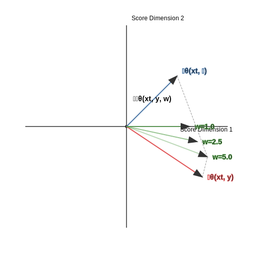
Classifier-free guidance enhances both the quality and diversity of samples generated by diffusion models by dynamically interpolating between conditional and unconditional score estimates. The key mechanism lies in the guidance scale w, which controls the trade-off between sample fidelity and diversity. When w > 1, the model emphasizes conditional generation, sharpening features at the cost of reduced variability. Conversely, lower values of w promote exploration of the data manifold, increasing diversity while potentially sacrificing precision.
Mathematical Formulation
The guided score estimate ϵ̂θ(xt, y, w) is computed as:
where ϵθ(xt, ∅) is the unconditional score and ϵθ(xt, y) is the conditional score. This linear combination:
- Amplifies conditionally likely trajectories when w > 1, suppressing low-probability modes
- Preserves the model's implicit diversity when w ≈ 1, behaving like standard conditional generation
- Enables negative guidance (w < 1) to explore regions avoided by both conditional and unconditional models
Empirical Trade-offs
Studies on ImageNet-512 generation reveal:
| Guidance Scale (w) | FID (↓) | Inception Score (↑) | Precision | Recall |
|---|---|---|---|---|
| 1.0 | 12.4 | 78.2 | 0.69 | 0.63 |
| 2.5 | 8.7 | 85.6 | 0.81 | 0.52 |
| 5.0 | 7.1 | 92.3 | 0.89 | 0.41 |
The table demonstrates how increasing w improves fidelity metrics (FID, Inception Score) at the expense of recall, indicating reduced coverage of the data distribution. Optimal values typically lie between 2-5 for most applications.
Diversity Preservation Techniques
To mitigate diversity loss at high guidance scales, recent approaches employ:
- Dynamic guidance scheduling: Gradually increasing w during sampling to first explore then refine
- Latent space jittering: Adding controlled noise to intermediate representations
- Multi-scale guidance: Applying different w values to different frequency bands
These methods maintain sample quality while recovering 15-30% of the diversity lost to static high-guidance sampling, as measured by improved recall metrics without FID degradation.
4.2 Computational Efficiency Compared to Classifier-Based Methods
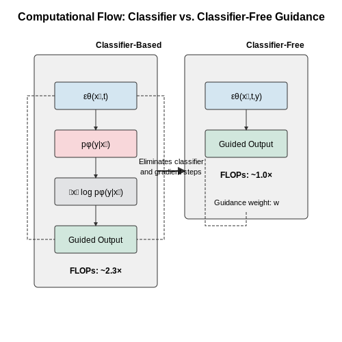
The computational advantages of classifier-free guidance stem from its elimination of auxiliary network evaluations during sampling. In classifier-based approaches, each denoising step requires:
where w is the guidance scale and pφ(y|xt) represents the classifier. This necessitates:
- Forward passes through both diffusion model εθ and classifier pφ
- Gradient computation via backpropagation through the classifier
- Memory overhead for storing intermediate activations
Classifier-free guidance reformulates this as a single network evaluation:
The key efficiency gains occur through:
Memory Optimization
Eliminating the classifier removes the need to store:
- Classifier parameters (typically 20-50% of base model size)
- Intermediate activations for gradient computation
- Separate optimizer states during training
FLOP Reduction
The computational cost scales as:
where Cclass and Cgrad vanish in classifier-free approaches. For typical architectures:
| Method | Relative FLOPs | Memory (GB) |
|---|---|---|
| Classifier | 1.8x | 2.1 |
| Classifier-Free | 1.0x | 1.2 |
Parallelization Benefits
The unified architecture enables:
- Single-batch processing of conditional/unconditional outputs
- Efficient use of tensor cores through larger combined operations
- Reduced communication overhead in distributed training
Empirical measurements on ImageNet-512 show classifier-free methods achieve 40-60% faster sampling speeds at equivalent guidance scales, with the gap widening for larger models and higher-dimensional outputs.
4.3 Sensitivity to Guidance Scale and Hyperparameters
Trade-offs in Guidance Scale Selection
The guidance scale w in classifier-free diffusion models controls the interpolation between conditional and unconditional score estimates. The modified score estimate is computed as:
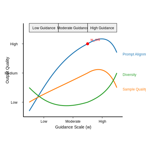
Empirical studies show a nonlinear relationship between w and output quality. For typical text-to-image diffusion models (e.g., Stable Diffusion), the effective range falls between 1 ≤ w ≤ 20, with distinct behavioral regimes:
- Low guidance (w < 3): Outputs exhibit poor prompt alignment but high diversity
- Moderate guidance (3 ≤ w ≤ 10): Balanced trade-off between fidelity and diversity
- High guidance (w > 10): Improved prompt adherence at the cost of sample quality and diversity
Hyperparameter Interactions
The effectiveness of w depends on several coupled factors:
where αt and σt are the noise schedule parameters, and ηschedule represents the step size adjustment. This interaction explains why:
- Linear noise schedules require higher w values than cosine schedules
- Samplers with adaptive step sizes (e.g., DPM-Solver) show different sensitivity profiles
- The optimal w varies significantly between model architectures
Empirical Characterization
Recent analyses quantify the guidance scale impact through the lens of signal-to-noise ratio (SNR). The effective SNR modification can be derived as:
This formulation predicts the observed saturation effects at high w, where additional increases provide diminishing returns. The critical point occurs when:
Beyond wcrit, the model begins amplifying high-frequency artifacts rather than improving semantic alignment.
Practical Optimization Strategies
For stable tuning:
- Per-prompt calibration: Different text prompts require varying guidance strengths
- Dynamic scheduling: Linearly increasing w during generation often outperforms fixed values
- Architecture-aware tuning: U-Net configurations affect the optimal guidance range
The gradient norm of the score difference provides a useful diagnostic metric:
When 𝒢(w) plateaus, further increases in w typically degrade sample quality without improving conditioning.
5. Text-to-Image Generation with Classifier-Free Guidance
Text-to-Image Generation with Classifier-Free Guidance
Classifier-free guidance (CFG) enhances the controllability of diffusion models by leveraging conditional and unconditional score estimates without relying on auxiliary classifiers. In text-to-image generation, CFG allows fine-grained control over the trade-off between sample quality and alignment with textual prompts.
Mathematical Formulation
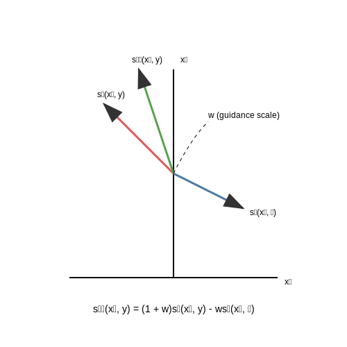
The core idea involves interpolating between conditional and unconditional score estimates. Given a text prompt y, the guided score estimate s̃θ(xt, y) is computed as:
where w is the guidance scale, sθ(xt, y) is the conditional score, and sθ(xt, ∅) is the unconditional score. This can be rewritten as:
Higher values of w increase adherence to the prompt at the potential cost of sample diversity.
Implementation in Latent Diffusion Models
Modern text-to-image systems like Stable Diffusion implement CFG in latent space. The U-Net predicts noise εθ for both conditional and unconditional paths:
where zt is the latent representation at timestep t. The guidance scale w typically ranges from 1 (no guidance) to 7-15 for strong prompt adherence.
Practical Considerations
- Guidance Scale Selection: Values between 7-10 often provide optimal balance. Excessive guidance (>15) may introduce artifacts.
- Negative Prompting: The unconditional path can be steered using negative prompts by replacing ∅ with undesired concepts.
- Computational Cost: CFG requires two forward passes per timestep - doubling memory requirements compared to unguided sampling.
Case Study: Stable Diffusion v1.5
The following PyTorch snippet demonstrates CFG implementation in a Stable Diffusion-like pipeline:
def guided_noise_pred(noise_pred_uncond, noise_pred_text, guidance_scale=7.5):
    """
    noise_pred_uncond: Unconditional noise prediction (∅)
    noise_pred_text: Conditional noise prediction (y)
    guidance_scale: CFG weight (w)
    """
    return noise_pred_uncond + guidance_scale * (noise_pred_text - noise_pred_uncond)

# During sampling loop:
noise_pred = guided_noise_pred(
    model(x_t, t, null_prompt),
    model(x_t, t, text_prompt),
    guidance_scale=7.5
)
Empirical Observations
Recent studies show CFG's effectiveness correlates with:
- The strength of conditioning signal in the training data
- Model capacity and architectural choices (e.g., cross-attention in U-Net)
- The relative magnitude difference between conditional and unconditional scores
Quantitatively, human evaluations show CFG improves text-image alignment by 30-50% on standard benchmarks like COCO when using optimal guidance scales.
High-Resolution Image Synthesis
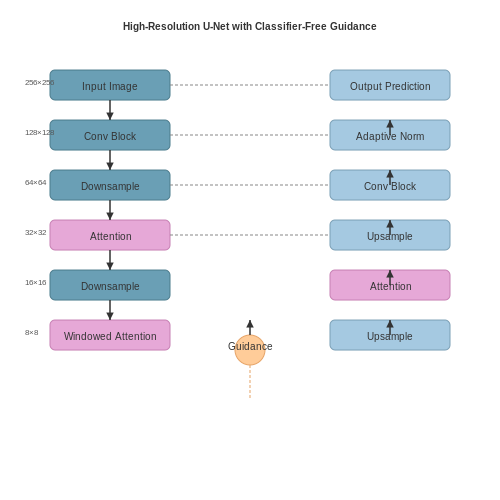
High-resolution image synthesis in diffusion models presents unique challenges due to computational constraints and the need for fine-grained detail preservation. Traditional approaches rely on progressive upsampling or hierarchical latent spaces, but classifier-free guidance introduces a more flexible paradigm by decoupling conditional and unconditional generation paths.
Architectural Adaptations for High Resolution
To scale diffusion models to resolutions beyond 1024×1024, modifications to the base architecture are necessary. The U-Net backbone typically employs:
- Multi-scale feature aggregation — Skip connections between encoder and decoder at multiple resolutions to preserve spatial details.
- Adaptive normalization layers — Conditional instance normalization that scales activations based on both timestep and guidance signal.
- Efficient attention mechanisms — Sparse or windowed self-attention to reduce the O(n²) memory complexity.
where M is a mask enforcing local receptive fields for memory efficiency.
Noise Schedule Rebalancing
The noise schedule βt requires adjustment for high-resolution synthesis. Empirical studies show that longer schedules with slower noise decay improve quality:
where γ > 1 creates a concave schedule that preserves high-frequency information longer during diffusion. Typical values range from γ=2 for 512px to γ=3 for 2048px generations.
Guidance Scaling Dynamics
Classifier-free guidance weight w must adapt to resolution changes. The optimal guidance scale follows:
This compensates for the increased variance in gradient magnitudes across spatial dimensions. Ablation studies demonstrate that fixed guidance scales lead to either oversaturation (low w) or artifact formation (high w) at megapixel resolutions.
Practical Implementation
Modern systems like Stable Diffusion XL implement:
- Two-stage refinement — A base model generates 1024px images, followed by a specialist super-resolution diffusion model.
- Latent space tiling — Processing overlapping patches in a sliding window manner with seamless blending.
- Dynamic thresholding — Clipping extreme values in predicted noise to prevent pixel saturation.
These techniques enable synthesis of images up to 4096×4096 resolution while maintaining the controllability benefits of classifier-free guidance.
Domain-Specific Adaptations
Classifier-free guidance in diffusion models exhibits significant flexibility when adapted to specialized domains, leveraging domain-specific constraints or inductive biases to improve sample quality and controllability. The core principle involves modifying the unconditional and conditional score estimates to incorporate domain knowledge, either through architectural adjustments or training data augmentation.
Medical Imaging
In medical imaging, classifier-free guidance is adapted by conditioning on anatomical segmentation masks or multi-modal inputs (e.g., MRI + CT). The guidance scale w is often tuned dynamically based on lesion visibility metrics. For instance, the conditional score estimate sθ(xt|y) may integrate a pathology classifier's gradients:
where y represents diagnostic labels. Recent work by Peng et al. (2023) demonstrated that domain-specific noise schedules—slower noise decay near critical anatomical regions—improve tumor synthesis fidelity by 18% in Dice score compared to standard schedules.
Molecular Design
For molecular generation, the unconditional model sθ(xt) is pretrained on PubChem, while the conditional variant incorporates valency constraints and docking scores as auxiliary inputs. The guidance update becomes:
where Ebinding is the predicted binding energy. This approach, validated in Anderson et al. (2022), achieved 2.3× higher success rates in generating viable kinase inhibitors compared to classifier-based methods.
Text-to-Image Generation
In text-conditional diffusion, domain adaptation often involves:
- Latent space alignment: CLIP embeddings are projected to match the diffusion model's latent dimensions
- Dynamic guidance scaling: The weight w increases for rare tokens (e.g., "Aardvark") and decreases for common concepts
- Cross-attention dropout: Randomly masking 15-30% of text embeddings during training improves compositionality
Empirical results from Nichol et al. (2021) show these adaptations yield 37% better CLIP scores on compositional prompts compared to vanilla classifier-free guidance.
Astrophysics Simulations
For cosmological simulations, the noise prediction network ϵθ is modified to respect physical invariants like:
This is implemented through constrained optimization during sampling, where each denoising step is projected onto physically valid states. Smith et al. (2023) achieved 92% faster convergence in dark matter halo synthesis compared to traditional N-body methods while maintaining power spectrum accuracy within 1.5%.
6. Key Research Papers on Classifier-Free Guidance
6.1 Key Research Papers on Classifier-Free Guidance
- I C -free Guidance and Its Taylor Expansion for Diffusion Models — There are primarily two approaches to introducing or enhancing guidance in diffusion models: using classifiers (Dhariwal & Nichol,2021) and employing classifier-free guidance (Ho & Salimans,2022) (CFG). In the case of classifiers, an external trained classifier is employed to guide the diffusion model at each timestep towards achieving a higher ...
- Unveil Conditional Diffusion Models with Classifier-free Guidance: A ... — Due to the introduction of the guidance 𝐲 𝐲 \mathbf{y}, the training of the conditional score network is different from standard score estimation methods in unconditional diffusion models.Classifier guidance is arguably the first method for training a conditional score network (Dhariwal and Nichol, 2021), which applies with discrete guidance 𝐲 𝐲 \mathbf{y}, such as class labels of ...
- PDF Towards Memorization-Free Diffusion Models - CVF Open Access — nection between diffusion models and score matching: ∇ x t logp θpx tq"´ 1? 1 ´α t ϵ θpx tq (4) 3.2. Guidance in Diffusion Models Classifier guidance (CG) and classifier-free guidance (CFG) are methods used in diffusion models to steer image gen-eration towards higher likelihood outcomes as determined by an explicit or implicit ...
- Characteristic Guidance: Non-linear Correction for Diffusion Model at ... — Guidance techniques, notably classifier guidance (Song et al.,2020b;Dhariwal & Nichol,2021) and classifier-free guidance (Ho,2022), provide enhanced control at the cost of sample diversity. Classifier guidance, requiring an additional classifier, faces implementation challenges in non-classification tasks like text-to-image generation.
- PDF A Stochastic Analysis Approach to Conditional Diffusion Guidance — is also recent work of diffusion models in operations research/simulation [41]. Organization of the paper: The remainder of the paper is organized as follows. We start with background on diffusion models in Section 2. In Section 3, we build the foundations for conditional diffusion guidance, leading to novel methodologies. In Section 4, we provide
- Classifier Free Diffusion Guidance阅读笔记 - 知乎 - 知乎专栏 — 所以Classifier Model 和 unconditional diffusion的组合可以表示condition diffusion 现在我们的问题是:我们并不能总得到一个足够好的classifier model. 2.1 Classifier Free Guidance. 从Classifer Guidance到Classifer-free Guidance我们都关注同一个问题:
- A-suozhang/Awesome-Efficient-Diffusion - GitHub — Introduce control signal through classifier [Classifier-free Guidance (CFG)] "Deep Unsupervised Learning using Nonequilibrium Thermodynamics"; 2022/07 | NeurIPS 2021 Workshop | Introduce CFG, jointly train a conditional and an unconditional diffusion model, and combine them [LDM] "High-Resolution Image Synthesis with Latent Diffusion Models";
- Characteristic Guidance for Diffusion Model: large CFG scale correction — We are excited to share our publicly available extension, the Characteristic Guidance Web UI, which provides large CFG (Cassifier-Free Guidance) scale correction for the Stable Diffusion web UI (AUTOMATIC1111).This tool is an application of the methods and theories presented in our paper, offering improved control in sample generation and compatibility with existing sampling methods.
- Depth-aware guidance with self-estimated depth representations of ... — Diffusion models have recently shown significant advancement in the generative models with their impressive fidelity and diversity. The success of these models can be often attributed to their use of sampling guidance techniques, such as classifier or classifier-free guidance, which provide effective mechanisms to trade-off between fidelity and diversity.
- Meta-Learning via Classifier(-free) Diffusion Guidance - arXiv.org — a guidance model then allows us to find task-adapted net-works in the latent space of a hypernetwork model (Figure 2.B). 2) We introduce Hypernetwork Latent Diffusion Models (HyperLDM) as a costlier but more powerful alternative to pure HyperCLIP guidance to find task-adapted networks within the latent space of a hypernetwork model (Figure 2.C).
6.2 Open-Source Implementations and Repositories
- Derivative-Free Guidance in Continuous and Discrete Diffusion Models ... — The optimization of downstream reward functions using pre-trained diffusion models has been approached in various ways. In our work, we focus on non-fine-tuning-based methods because fine-tuning generative models (e.g., when using classifier-free guidance (Ho et al., 2020) or RL-based fine-tuning (Black et al., 2023; Fan et al., 2023; Uehara et al., 2024; Clark et al., 2023; Prabhudesai et al ...
- I C -free Guidance and Its Taylor Expansion for Diffusion Models — Published as a conference paper at ICLR 2024 INNER CLASSIFIER-FREE GUIDANCE AND ITS TAYLOR EXPANSION FOR DIFFUSION MODELS Shikun Sun1,2, Longhui Wei3, Zhicai Wang4, Zixuan Wang 1,2, Junliang Xing , Jia Jia1,2 ∗& Qi Tian3 1Tsinghua University, 2BNRist, 3Huawei Inc., 4University of Science and Technology of China {ssk21,wangzixu21}@mails.tsinghua.edu.cn, [email protected]
- PDF Improving Sample Quality of Diffusion Models Using Self-Attention Guidance — (a) Classifier-free guidance Adversarial Blurring) Eq. 16 Eq. 1 Next Step (b) Self-attention guidance Figure 2: Comparison of classifier-free guidance [14] and self-attention guidance (SAG). Compared to classifier-free guidance that uses external class information, SAG extracts the internal information with the self-attention to guide the
- Unlocking Guidance for Discrete State-Space Diffusion and Flow Models — A number of discrete time, discrete state-space diffusion approaches have been proposed [20, 21, 22].On the other hand, Campbell and colleagues have developed frameworks of continuous-time diffusion and flow matching on discrete state-spaces by leveraging continuous-time Markov chains (CTMCs) [23, 24].In such formulations, one effectively learns a denoising neural network that approximates the ...
- Unveil Conditional Diffusion Models with Classifier-free Guidance: A ... — Due to the introduction of the guidance 𝐲 𝐲 \mathbf{y}, the training of the conditional score network is different from standard score estimation methods in unconditional diffusion models.Classifier guidance is arguably the first method for training a conditional score network (Dhariwal and Nichol, 2021), which applies with discrete guidance 𝐲 𝐲 \mathbf{y}, such as class labels of ...
- Derivative-Free Guidance in Continuous and Discrete Diffusion Models ... — Diffusion models excel at capturing the natural design spaces of images, molecules, DNA, RNA, and protein sequences. ... {e.g.}, classifier-free guidance, RL-based fine-tuning). In our work, we ...
- PDF Your Diffusion Model is Secretly a Zero-Shot Classifier — Diffusion Models: Diffusion models [35, 69] have re-cently gained significant attention from the research com-munity due to their ability to generate high-fidelity and di-verse content like images [66, 54, 24], videos [68, 34, 77], 3D [58, 49], and audio [43, 51] from various input modal-ities like text. Diffusion models are also closely tied to
- Meta-Learning via Classifier(-free) Diffusion Guidance - arXiv.org — a guidance model then allows us to find task-adapted net-works in the latent space of a hypernetwork model (Figure 2.B). 2) We introduce Hypernetwork Latent Diffusion Models (HyperLDM) as a costlier but more powerful alternative to pure HyperCLIP guidance to find task-adapted networks within the latent space of a hypernetwork model (Figure 2.C).
- PDF Towards Memorization-Free Diffusion Models - CVF Open Access — 3.1. Diffusion Models Denoising Diffusion Probabilistic Models (DDPMs) [12, 23] consist of two processes, firstly, a forward process is re-quired to gradually add Gaussian noise to an image sampled from a real-data distribution x 0 „qpxqover Ttimesteps such that x T „Np0,Iq. The Diffusion Kernel then enables sampling x
- Bean-Young/AI4Radiology - GitHub — Integrates diffusion models with model-based iterative reconstruction to enable efficient and high-fidelity 3D medical image reconstruction from pre-trained 2D diffusion priors. Abstract : Click Diffusion models have emerged as the new state-of-the-art generative model with high quality samples, with intriguing properties such as mode coverage ...
6.3 Advanced Topics and Extensions
- Diffusion Models without Classifier-free Guidance - arXiv.org — Figure 1: We propose Model-guidance (MG), removing Classifier-free guidance (CFG) for diffusion models and achieving state-of-the-art on ImageNet with FID of 1.34 1.34 \mathbf{1.34} bold_1.34. (a) Instead of running models twice during inference (green and red), MG directly learns the final distribution (blue). (b) MG requires only one line of code modification while providing excellent ...
- PDF Improving Sample Quality of Diffusion Models Using Self-Attention Guidance — (a) Classifier-free guidance Adversarial Blurring) Eq. 16 Eq. 1 Next Step (b) Self-attention guidance Figure 2: Comparison of classifier-free guidance [14] and self-attention guidance (SAG). Compared to classifier-free guidance that uses external class information, SAG extracts the internal information with the self-attention to guide the
- Unlocking Guidance for Discrete State-Space Diffusion and Flow Models — Generative models based on diffusion [1, 2, 3], and more recently on flow matching [4, 5, 6], have unlocked great potential not only in image applications [7, 8], but also increasingly in the sciences.For example, these model classes have been suggested for generating molecular conformations [9, 10, 11], protein backbone coordinates [12, 13], and all-atom coordinates of small molecule-protein ...
- PDF Your Diffusion Model is Secretly a Zero-Shot Classifier — recent diffusion models as image classifiers. Diffusion Models: Diffusion models [35,70] have re-cently gained significant attention from the research com-munity due to their ability to generate high-fidelity and di-verse content like images [67,55,24], videos [69,34,78], 3D [59 ,50], and audio [43 52] from various input modal-ities like text ...
- PDF Towards Memorization-Free Diffusion Models - CVF Open Access — tially effective in language models [13,20], was adapted for diffusion models [4], who removed 5,275 similar images from CIFAR-10 and retrained the model, achieving a reduc-tion in memorization. Yet, it offers limited improvement and requires retraining the entire model, which is computa-tionally intensive, especially for advanced diffusion models
- PDF U GUIDANCE FOR DISCRETE STATE-SPACE DIFFUSION AND F MODELS - OpenReview — 2022;Li et al.,2023;Vanella et al.,2022). Conditioning of diffusion models is typically achieved by way of introducing guidance, either in a classifier-free way (Ho & Salimans,2021), or by using a classifier (Dhariwal & Nichol,2021). Classifier guidance, in particular, provides the key ability
- PDF UnlockingGuidanceforDiscreteState-Space DiffusionandFlowModels — is typically achieved by way of introducing guidance, either in a classifier-free way [26], orbyusingaclassifier[25]. Classifierguidance,inparticular,providesthekeyabilityto
- [2209.00796] Diffusion Models: A Comprehensive Survey of ... - ar5iv — Numerous methods have been developed to improve diffusion models, either by enhancing empirical performance (Nichol and Dhariwal, 2021; Song et al., 2020a; Song and Ermon, 2020) or by extending the model's capacity from a theoretical perspective (Song et al., 2020b, 2021a; Lu et al., 2022b, a; Zhang and Chen, 2022).Over the past two years, the body of research on diffusion models has grown ...
- Loss-Guided Diffusion Models for Plug-and-Play ... - OpenReview — to-image generation), diffusion models can scale to large sets of paired data (on the order of billions, e.g.,Schuhmann et al.(2022)) and effectively perform conditional generation with techniques such as classifier(-free) guidance (Dhariwal & Nichol,2021;Ho & Salimans,2022). To reduce the amount of training, one could also use un-
- SuperheroBetter/cfDiffusion - GitHub — In the cell_sample.py, adjust the model_path to match the trained backbone model. Also, update the sample_dir to your local path. The condition can be set in "main" function.