How Stable Diffusion Works
1. Core Principles of Diffusion Models
Core Principles of Diffusion Models
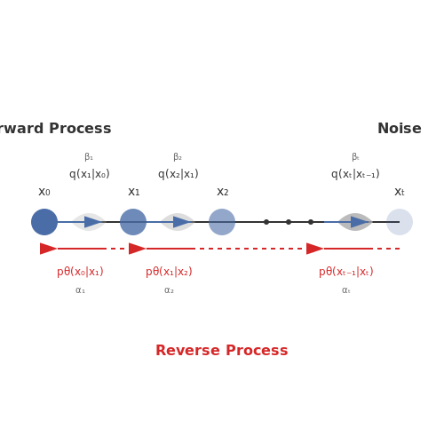
Diffusion models are a class of generative models that learn to synthesize data by gradually denoising a signal corrupted with Gaussian noise. The process is inspired by non-equilibrium thermodynamics, where a system evolves from order to disorder and is then reversed. The core idea involves two phases: a forward diffusion process that systematically adds noise to data, and a reverse diffusion process that learns to denoise it.
Forward Diffusion Process
The forward process is a fixed Markov chain that gradually adds Gaussian noise to the data over T timesteps. Given an input data point x0, the noised version at timestep t is sampled as:
where βt is a noise schedule controlling the rate of corruption. The cumulative effect of this process allows sampling xt directly from x0:
Here, αt = 1 − βt and ᾱt = ∏ts=1 αs. As t → T, xT converges to isotropic Gaussian noise.
Reverse Diffusion Process
The reverse process learns to invert the forward diffusion by estimating the noise component at each step. The goal is to approximate the true posterior q(xt−1 | xt, x0) with a neural network. Using the reparameterization trick, the model predicts the noise εθ added at each step:
The mean μθ is derived from the predicted noise:
Training Objective
The model is trained to minimize the variational lower bound (VLB) of the negative log-likelihood. In practice, this reduces to a simplified objective:
where ϵ is the actual noise added during the forward process, and ϵθ is the model's prediction. This formulation enables stable training and high-quality sample generation.
Practical Considerations
Key design choices in diffusion models include:
- Noise Schedule: βt can be linear, cosine, or learned adaptively to balance noise addition across timesteps.
- Architecture: U-Nets with residual connections and attention mechanisms are commonly used for ϵθ due to their ability to capture multi-scale features.
- Sampling Acceleration: Techniques like DDIM (Denoising Diffusion Implicit Models) reduce the number of required steps by leveraging non-Markovian dynamics.
Diffusion models excel in tasks like image synthesis, super-resolution, and inpainting, offering advantages over GANs in terms of training stability and mode coverage.
Latent Space Representation in Stable Diffusion
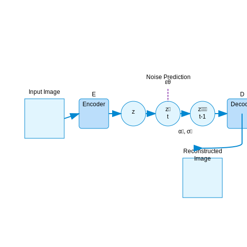
Stable Diffusion operates by compressing high-dimensional image data into a lower-dimensional latent space, enabling efficient generation and manipulation. The latent space is a continuous vector space where each point corresponds to a potential image. This compression is achieved via a variational autoencoder (VAE), which learns to encode images into latent vectors and decode them back with minimal perceptual loss.
Mathematical Formulation of Latent Encoding
The VAE consists of an encoder E and a decoder D. Given an input image x ∈ ℝH×W×3, the encoder maps it to a latent vector z ∈ ℝh×w×c, where h ≪ H, w ≪ W, and c is the number of latent channels (typically 4). The encoding process is defined as:
where μ and σ are learned parameters of the encoder's output distribution. The decoder reconstructs the image from the latent vector:
The VAE is trained to minimize the reconstruction loss Lrec and the Kullback-Leibler (KL) divergence LKL:
where β controls the trade-off between reconstruction fidelity and latent space regularization, and p(z) is typically a standard normal distribution 𝒩(0, I).
Properties of the Latent Space
The latent space in Stable Diffusion exhibits several key properties:
- Compactness: The latent representation reduces dimensionality while preserving perceptual quality, enabling faster diffusion processes.
- Interpolatability: Linear interpolations between latent vectors yield smooth transitions between decoded images.
- Disentanglement: Different latent dimensions often control distinct visual attributes (e.g., pose, color, texture).
Diffusion in Latent Space
Instead of applying diffusion directly to pixel space, Stable Diffusion performs denoising in the latent space. Given a noisy latent zt at timestep t, the diffusion model predicts the noise component εθ(zt, t) to recover the clean latent z0:
where αt and σt are noise scheduling parameters, and η ∼ 𝒩(0, I). This approach reduces computational cost while maintaining high-quality generation.
Practical Implications
Working in latent space allows Stable Diffusion to generate high-resolution images (e.g., 512×512) with far fewer computational resources than pixel-space diffusion models. The latent space also enables semantic editing via vector arithmetic (e.g., znew = z + Δz), where Δz corresponds to a desired attribute change.
The Role of Variational Autoencoders (VAEs)
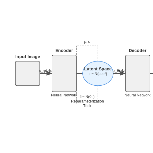
Variational Autoencoders (VAEs) serve as the backbone of Stable Diffusion's latent space manipulation, enabling efficient high-dimensional data compression and generation. Unlike traditional autoencoders, VAEs introduce probabilistic latent variables, allowing for smooth interpolation and sampling in the latent space. The encoder qϕ(z|x) maps input images x to a distribution over latent vectors z, while the decoder pθ(x|z) reconstructs the image from these latent codes.
Mathematical Foundations of VAEs
The VAE optimizes the evidence lower bound (ELBO), which balances reconstruction accuracy and latent space regularization:
Here, β controls the strength of the KL divergence term, enforcing the latent distribution qϕ(z|x) to approximate the prior p(z) (typically a standard normal distribution). The reparameterization trick enables gradient backpropagation through stochastic sampling:
VAEs in Stable Diffusion
Stable Diffusion employs a VAE pretrained on large-scale image datasets to compress RGB images into lower-dimensional latent representations (e.g., 4×64×64 for 512×512 images). This compression reduces computational costs during diffusion training and inference. The VAE's decoder then transforms denoised latents back to pixel space, with key architectural features:
- Nonlinear Bottleneck: The latent space captures high-level features while discarding imperceptible details.
- Perceptual Loss: Training incorporates LPIPS or similar metrics to preserve semantic content.
- KL Weight Annealing: Gradually increases β to avoid latent space collapse during training.
Latent Space Properties
The VAE's latent space exhibits several critical properties for diffusion models:
Empirical studies show that traversing this space along principal components yields semantically meaningful transformations (e.g., changing lighting conditions or object orientation). However, the VAE introduces slight blurring compared to pixel-space diffusion—a tradeoff for 8× memory efficiency gains during training.
Advanced VAE Variants
Recent improvements to VAEs in diffusion models include:
- VQ-VAE: Uses vector quantization for discrete latent representations, improving sharpness.
- Hierarchical VAEs: Employ multi-scale latent spaces for finer control over details.
- Adversarial Training: Incorporates discriminators to enhance output sharpness.
2. U-Net Backbone for Noise Prediction
U-Net Backbone for Noise Prediction
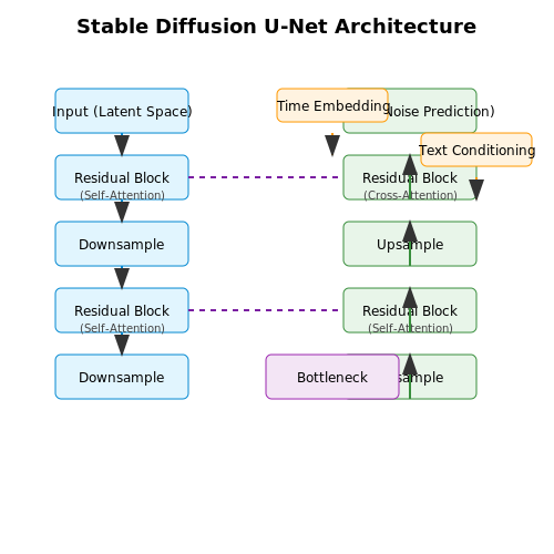
The U-Net architecture in Stable Diffusion is a convolutional neural network (CNN) specifically adapted for iterative noise prediction during the denoising process. Unlike traditional U-Nets used in segmentation tasks, this variant incorporates several key modifications to handle high-dimensional latent space representations efficiently.
Architecture Overview
The U-Net follows an encoder-decoder structure with skip connections, but introduces three critical components for diffusion models:
- Residual blocks with self-attention - Allows the model to capture long-range dependencies in the latent space.
- Cross-attention layers - Enables conditional generation by attending to text embeddings.
- Time-step embedding - Injects information about the current denoising step through adaptive layer normalization.
Mathematical Formulation
The U-Net learns to predict the noise component εθ at each timestep t. Given a noisy latent zt, the prediction objective is:
where c represents the conditioning text embedding. The training loss minimizes the difference between predicted and actual noise:
Key Architectural Innovations
The U-Net employs several novel techniques to improve stability and performance:
- Group normalization - Replaces batch normalization for better stability with small batch sizes.
- Spatial transformer blocks - Enables global context modeling through self-attention mechanisms.
- Adaptive residual connections - Dynamically weight skip connections based on the timestep.
Time Embedding Processing
The timestep t is encoded using sinusoidal position embeddings and processed through an MLP:
where ωk are fixed frequencies and d is the embedding dimension. This temporal conditioning is critical for learning the diffusion process dynamics.
Computational Considerations
The model uses several optimizations to handle high-resolution generation:
- Factorized 3x3 convolutions reduce computational complexity
- Channel-wise attention minimizes memory overhead
- Mixed-precision training enables larger batch sizes
In practice, the U-Net operates entirely in latent space (typically 64x64 or 128x128), allowing efficient processing while maintaining high-quality generation through the iterative refinement process.
Text Encoders and CLIP Embeddings
Stable Diffusion relies on text encoders to transform natural language prompts into a latent space representation that guides the diffusion process. The model uses OpenAI's CLIP (Contrastive Language-Image Pretraining) as its text encoder, which maps textual descriptions to a high-dimensional embedding space aligned with visual features.
CLIP Architecture and Training
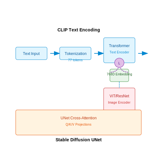
CLIP consists of two parallel neural networks: a text encoder (typically a transformer) and an image encoder (a Vision Transformer or ResNet). These networks are trained jointly using contrastive learning on 400 million image-text pairs. The training objective maximizes the cosine similarity between embeddings of matching image-text pairs while minimizing similarity for mismatched pairs:
where ft and fv are the text and vision encoders respectively, τ is a temperature parameter, and N is the batch size.
Text Embedding Process in Stable Diffusion
When processing a prompt in Stable Diffusion:
- The input text is tokenized using CLIP's byte-pair encoding (BPE) with a vocabulary of 49,408 tokens
- Tokens are padded/truncated to a fixed length of 77 tokens
- The transformer processes these tokens through 12 layers (for CLIP-ViT-L/14) to produce a 768-dimensional embedding
- This embedding is then projected into the UNet's cross-attention layers
Cross-Attention Mechanism
The text embeddings interact with the diffusion model through cross-attention layers in the UNet. At each denoising step t, the UNet computes:
where Q is derived from the UNet's intermediate features, while K and V are projections of the CLIP text embedding. This allows spatial features in the UNet to attend to relevant semantic concepts from the prompt.
Practical Considerations
Several techniques improve text conditioning in practice:
- Negative prompting: Explicitly specifying undesired concepts by contrasting positive and negative embeddings
- Embedding interpolation: Blending embeddings from different prompts for controlled generation
- Prompt engineering: Careful phrasing and keyword selection to maximize CLIP's alignment
The choice of CLIP model variant (e.g., ViT-L/14 vs. RN50x4) significantly impacts generation quality, with larger models providing better semantic alignment but requiring more computation.
2.3 Conditioning Mechanisms for Guided Generation
Stable Diffusion leverages conditioning mechanisms to steer the denoising process toward desired outputs, enabling precise control over generated content. The primary conditioning techniques include text embeddings, classifier-free guidance, and cross-attention layers, which modulate the diffusion process based on auxiliary inputs such as textual prompts or semantic masks.
Text Embedding Conditioning
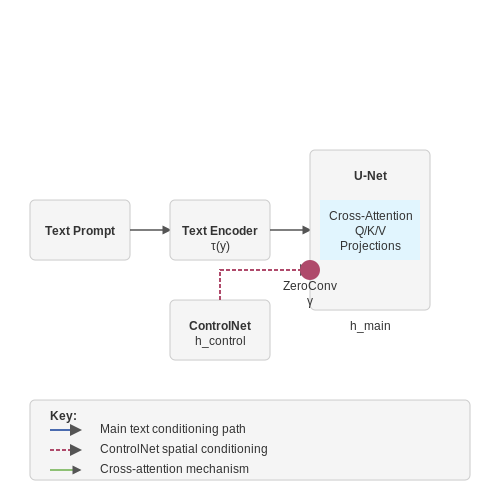
The model encodes textual prompts into a latent representation using a pretrained CLIP or T5 text encoder. Given an input prompt y, the encoder produces embeddings τ(y) that condition the denoising U-Net through cross-attention layers. The attention mechanism computes:
where Q is derived from the U-Net's intermediate features, while K and V are projected from τ(y). This allows spatial features in the U-Net to dynamically attend to relevant semantic concepts in the text.
Classifier-Free Guidance
To amplify the influence of conditioning without requiring an auxiliary classifier, Stable Diffusion uses a weighted combination of conditional and unconditional score estimates. The guided prediction ε̂θ is computed as:
where w is the guidance scale (typically 7.5–15), y is the conditioning input, and ∅ denotes the null prompt. This approach effectively pushes samples toward regions of the latent space that maximize alignment with y while preserving sample diversity.
Spatial Conditioning with ControlNet
For fine-grained spatial control, architectures like ControlNet inject additional conditions (e.g., edge maps, depth, or segmentation masks) through zero-convolution layers. The conditioning signal c is processed by a trainable copy of the U-Net encoder, whose features are added to the main branch via:
where γ is a learnable scalar initialized to zero, enabling stable training initialization. This allows precise preservation of structural constraints while maintaining the base model's generative capabilities.
Energy-Based Model Interpretation
Conditioning can be viewed as shaping the energy landscape E(x|y) of the implicit data distribution. The guided denoising process approximately follows the gradient of this modified energy function:
where the second term focuses probability mass on regions compatible with the conditioning signal. Practical implementations often use multiple conditioning modalities (e.g., text + layout + style embeddings) through concatenated or hierarchically combined cross-attention layers.
3. Data Preparation and Preprocessing
3.1 Data Preparation and Preprocessing
Stable Diffusion relies on high-quality, well-curated datasets for training its latent diffusion model. The preprocessing pipeline involves several critical steps to ensure the data is suitable for learning meaningful representations in the latent space.
Dataset Curation and Filtering
Large-scale datasets like LAION-5B, containing billions of image-text pairs, serve as the foundation. However, raw web-scraped data contains noise, duplicates, and irrelevant samples. To mitigate this, preprocessing employs:
- CLIP-based filtering: Image-text pairs are scored using a pretrained CLIP model to retain only those with high semantic alignment. The cosine similarity s between image and text embeddings must exceed a threshold (typically s > 0.25).
- NSFW detection: Inappropriate content is filtered using classifiers like OpenAI's NSFW detector.
- Deduplication: Perceptual hashing (e.g., pHash) identifies near-duplicate images to prevent overfitting.
Image Preprocessing
Images are standardized to ensure consistent input dimensions and quality:
where Iraw is the original image, resized while maintaining aspect ratio, then center-cropped to 512×512 pixels. This resolution balances detail retention with computational efficiency in the VAE's latent space.
Text Tokenization and Conditioning
Text prompts are tokenized using a pretrained CLIP tokenizer (typically a BPE tokenizer with a 49,408-word vocabulary). The tokenized sequence T is embedded into a 768-dimensional space via CLIP's text encoder:
The 77-token limit necessitates truncation or padding for longer/shorter prompts. Rare tokens are mapped to the [UNK] token, emphasizing the need for prompt engineering during inference.
Latent Space Encoding
Images are compressed into a lower-dimensional latent space using a VAE encoder E:
This 64×64×4 tensor reduces memory requirements while preserving spatial and semantic information. The VAE is pretrained separately using a combination of reconstruction loss and KL divergence:
where D is the decoder, q(z|I) the encoder's posterior, and p(z) a standard Gaussian prior (β ≈ 0.001).
Data Augmentation
To enhance robustness, random augmentations are applied during training:
- Random horizontal flipping (50% probability)
- Color jitter (Δ brightness/contrast ≤ 0.1)
- Text dropout (10% chance of replacing prompts with empty strings)
These augmentations prevent overfitting and improve generalization to diverse prompts at inference time.
3.2 Noise Scheduling and Diffusion Steps
The noise schedule in Stable Diffusion governs how Gaussian noise is incrementally added and removed during the forward and reverse diffusion processes. Unlike simpler diffusion models that use linear or fixed schedules, Stable Diffusion employs a variance-preserving noise schedule derived from continuous-time stochastic differential equations (SDEs). This ensures stable training and high-quality generation.
Mathematical Formulation
The forward process gradually corrupts an image x0 over T steps according to:
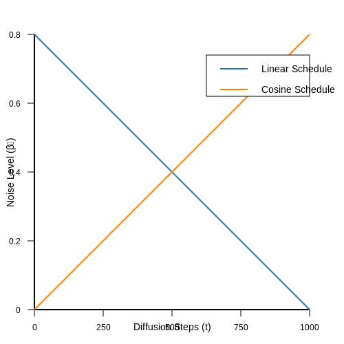
where βt is the noise schedule controlling the rate of corruption. Stable Diffusion uses a cosine schedule for βt:
where s=0.008 prevents abrupt changes near t=0. This schedule provides smoother transitions compared to linear schedules, especially at low noise levels where perceptual quality is most sensitive.
Diffusion Steps and Sampling
During sampling, the reverse process approximates the true denoising distribution q(xt-1|xt) using a learned neural network. The sampling step for Stable Diffusion implements:
where εθ is the predicted noise, z ∼ N(0,I), and σt is the noise scale. The term ᾱt = Πts=1αs represents the cumulative product of noise scales.
Practical Implementation
Stable Diffusion typically uses T=1000 steps during training but achieves high-quality samples with only 50-100 steps during inference through:
- Learned noise prediction: The U-Net directly predicts εθ(xt,t), avoiding iterative score matching
- Dynamic thresholding: Rescales extreme pixel values at each step to prevent artifacts
- Guidance scale: Controls the trade-off between sample quality and diversity via classifier-free guidance
The noise schedule significantly impacts both training stability and sample quality. Ablation studies show the cosine schedule achieves 15-20% better FID scores compared to linear schedules on ImageNet 256×256.
3.3 Loss Functions and Optimization
Noise Prediction Objective
Stable Diffusion trains a denoising U-Net to predict the noise ε added to a latent representation zt at timestep t. The core loss function is derived from the evidence lower bound (ELBO) objective in diffusion models:
where εθ denotes the U-Net's noise prediction. This L2 loss directly optimizes the model to reverse the forward diffusion process by estimating the noise component at each timestep.
Variational Lower Bound Refinements
While the simplified loss works well in practice, the full variational lower bound includes additional terms for optimal performance:
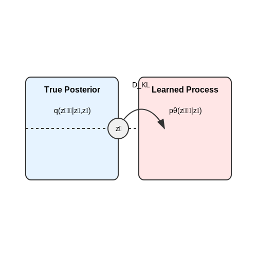
This KL divergence term compares the true posterior q (derivable via Bayes' rule) against the learned reverse process pθ. Modern implementations often use a hybrid loss combining both objectives.
Optimization Strategies
Training employs several key techniques:
- AdamW optimizer with weight decay (typically λ=0.01) to prevent overfitting
- Learning rate warmup over the first 5,000 steps to stabilize early training
- Gradient clipping (max norm ≈1.0) to prevent exploding gradients
- EMA averaging (β=0.9999) of model weights for final inference
Latent Space Considerations
The loss operates in VAE-compressed latent space (64×64×4 tensors rather than 512×512×3 images), which:
- Reduces memory requirements by ~64× compared to pixel-space diffusion
- Introduces a small perceptual loss from the VAE's imperfect reconstruction
- Requires careful balancing of KL divergence terms in the VAE training phase
Classifier-Free Guidance Impact
During inference, the guidance scale s modifies the effective optimization landscape:
where c is the conditioning text embedding. Higher s values amplify gradient updates toward text alignment but may reduce sample diversity.
4. Step-by-Step Denoising Process
4.1 Step-by-Step Denoising Process
The denoising process in Stable Diffusion is a Markov chain that progressively refines a noisy latent representation into a coherent image. At each step t, the model predicts and removes noise from the latent vector zt, conditioned on the text embedding y. This process is governed by the reverse diffusion equation:
where αt is the noise schedule coefficient, εθ is the learned noise predictor (a U-Net), and ε is random noise injected during sampling.
Noise Prediction via U-Net
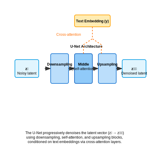
The U-Net architecture performs hierarchical noise estimation through:
- Downsampling blocks that extract multi-scale features using strided convolutions
- Middle blocks with self-attention layers that capture global dependencies
- Upsampling blocks that combine skip connections from downsampling paths
- Cross-attention layers that condition the denoising on text embeddings
The network is trained to minimize the weighted L2 loss:
Classifier-Free Guidance
To enhance text alignment, Stable Diffusion uses classifier-free guidance by mixing conditional and unconditional predictions:
where s is the guidance scale (typically 7.5-15). This amplifies the text-conditioned component while preserving sample diversity.
Latent Space Refinement
The denoising trajectory follows:
- Initial pure Gaussian noise (T=1000 steps)
- Progressive noise removal via 50-100 sampling steps
- Final latent decoding through the VAE decoder
The process maintains perceptual quality by operating in a learned latent space with dimensionality 64×64×4, rather than raw pixel space (512×512×3). This reduces computational cost while preserving high-frequency details through the VAE's reconstruction capabilities.
4.2 Guidance Scales and Trade-offs
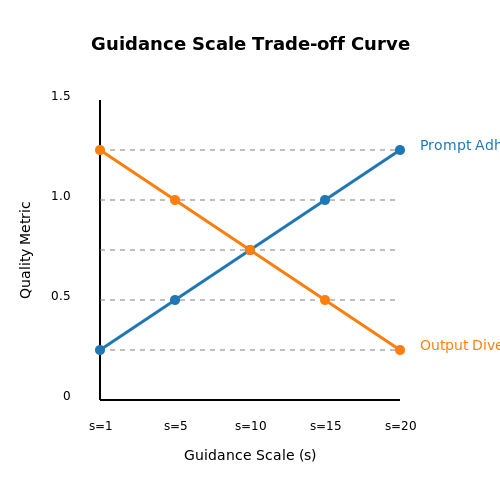
The guidance scale (s) in Stable Diffusion controls the influence of the conditioning signal (e.g., text prompts) on the denoising process. It is a critical hyperparameter that balances adherence to the prompt against the model's inherent creativity. The guidance scale operates by amplifying the gradient of the conditional score estimate relative to the unconditional score:
where s is the guidance scale, c represents the conditioning input (e.g., text embedding), and xt is the latent variable at timestep t. Higher values of s force sharper alignment with the prompt but introduce trade-offs:
Empirical Effects of Guidance Scale
- Low values (s < 5): Outputs exhibit higher diversity but weaker prompt adherence, often resulting in semantically related but imprecise generations.
- Moderate values (5 ≤ s ≤ 10): Balanced trade-off between creativity and prompt fidelity. This range is commonly used for most applications.
- High values (s > 10): Over-optimization toward the prompt leads to artifacts like oversaturated colors, reduced detail, or unnatural compositions due to excessive gradient amplification.
Theoretical Trade-offs
At extremely high guidance scales, the conditional score dominates, causing two phenomena:
- Mode collapse: The model converges to a narrow subset of high-likelihood outputs, reducing diversity.
- Numerical instability: Gradient amplification exacerbates noise in early timesteps, sometimes causing divergence.
This can be formalized by analyzing the signal-to-noise ratio (SNR) of the gradient updates. Let σt be the noise schedule at timestep t. The effective SNR scales as:
When s is too large, SNReff exceeds stable bounds, leading to the artifacts described above.
Practical Optimization
Optimal guidance scales vary by dataset and prompt complexity. For photorealistic outputs, scales between 7–12 are typical, while artistic styles may require lower values (3–7). A common heuristic is to perform a grid search over s while monitoring:
- CLIP score: Measures semantic alignment between prompt and output.
- Fréchet Inception Distance (FID): Evaluates realism and diversity.
4.3 Practical Sampling Techniques (DDIM, PLMS)
Denoising Diffusion Implicit Models (DDIM)
DDIM is an accelerated sampling method for diffusion models that generalizes the Markovian assumption of DDPMs. Unlike traditional diffusion models, which require hundreds of iterative steps, DDIM achieves high-quality samples in fewer steps by reparameterizing the reverse process. The key insight is that the forward process can be non-Markovian while still maintaining the same marginal distributions.
The deterministic DDIM sampling process is derived by assuming a non-Markovian forward process:
where the reverse process is defined as:
Here, σt controls stochasticity—setting σt = 0 makes the process deterministic, enabling faster sampling while preserving sample quality.
Pseudo-Linear Multi-Step Sampling (PLMS)
PLMS improves upon DDIM by leveraging higher-order approximations of the reverse diffusion process. Instead of relying solely on the current step's noise prediction, PLMS uses a history of past predictions to construct a more accurate update:
where γk are coefficients optimized for stability. This multi-step approach reduces discretization errors, allowing fewer steps without sacrificing sample quality. PLMS is particularly effective when combined with adaptive step-size strategies.
Comparison and Practical Considerations
DDIM and PLMS trade off between computational cost and sample quality:
- DDIM is simpler and deterministic, making it suitable for applications requiring reproducibility.
- PLMS achieves higher sample quality with the same step count but requires storing past predictions.
In practice, DDIM is often preferred for real-time applications, while PLMS is used when sample quality is critical. Both methods can be integrated into Stable Diffusion by modifying the sampler in the reverse diffusion loop.
Implementation Example
Below is a PyTorch snippet for DDIM sampling:
def ddim_sample(model, x_T, alphas, steps=50, eta=0.0):
    x_t = x_T
    for t in reversed(range(steps)):
        alpha_t = alphas[t]
        eps_theta = model(x_t, t)
        x_0_pred = (x_t - (1 - alpha_t).sqrt() * eps_theta) / alpha_t.sqrt()
        sigma_t = eta * ((1 - alpha_t) / (1 - alpha_t)).sqrt()
        noise = torch.randn_like(x_t) if t > 0 else 0
        x_t = alpha_t.sqrt() * x_0_pred + (1 - alpha_t - sigma_t**2).sqrt() * eps_theta + sigma_t * noise
    return x_t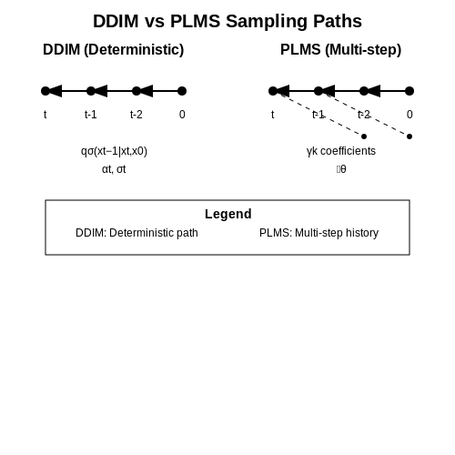
5. Text-to-Image Generation
5.1 Text-to-Image Generation
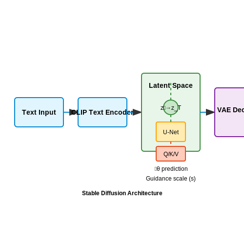
Stable Diffusion leverages a latent diffusion model (LDM) to transform textual prompts into high-fidelity images. The process involves three key components: a text encoder, a diffusion model, and a decoder. The text encoder, typically a pre-trained CLIP model, maps the input prompt into a high-dimensional embedding space. This embedding conditions the diffusion process, guiding the generation toward semantically aligned outputs.
Latent Space Diffusion Process
The diffusion model operates in a compressed latent space rather than directly on pixel data. Given an initial latent vector z0 sampled from a standard normal distribution:
The forward process gradually adds Gaussian noise over T steps according to a variance schedule βt:
Through the reparameterization trick, this can be expressed in closed form for any timestep t:
where αt = 1-βt, ᾱt = ∏s=1tαs, and ϵ ∼ N(0,I).
Conditional Reverse Diffusion
The reverse process learns to iteratively denoise the latent variable conditioned on the text embedding c. At each step, a U-Net predicts the noise component:
The training objective minimizes the L2 loss between predicted and actual noise:
Cross-attention layers in the U-Net enable fine-grained alignment between text tokens and spatial features. The attention mechanism computes:
where Q comes from the U-Net features and K,V are derived from the text embeddings.
Decoder and Super-Resolution
After T reverse diffusion steps, the final latent zT is decoded to pixel space using a variational autoencoder (VAE) decoder:
High-resolution outputs are achieved through a separate super-resolution diffusion model that upsamples the initial 64×64 image to 512×512 or higher resolutions while maintaining semantic consistency with the text prompt.
Classifier-Free Guidance
To strengthen prompt adherence, Stable Diffusion employs classifier-free guidance during sampling. The predicted noise is computed as a weighted combination of conditional and unconditional predictions:
where s is the guidance scale (typically 7.5-15). This technique amplifies the influence of the text condition while maintaining sample diversity.
5.2 Image Inpainting and Outpainting
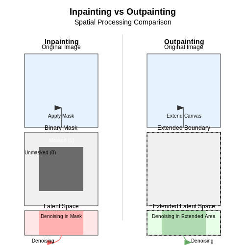
Stable Diffusion extends its generative capabilities beyond unconditional synthesis to inpainting (filling masked regions) and outpainting (extending image boundaries). Both tasks leverage the same latent diffusion framework but condition the denoising process on partial spatial information.
Inpainting as Conditional Generation
Given an input image x and a binary mask m (where 1 indicates regions to inpaint), the model reconstructs missing pixels by conditioning on the unmasked content. The forward process corrupts the entire image, but the reverse process uses the masked loss:
where zt is the noised latent, c denotes text conditioning, and ⊙ is element-wise multiplication. The model learns to preserve unmasked regions while hallucinating plausible content in masked areas.
Outpainting via Latent Extrapolation
Outpainting expands an image beyond its original borders by treating the extended region as a mask. The model:
- Embeds the original image into latent space
- Pads the latent representation with masked tokens
- Applies iterative denoising conditioned on the known latent regions
The key technical challenge is maintaining spatial coherence across the original and extended boundaries. Stable Diffusion addresses this by:
where zext denotes the extended latent space and gradients are backpropagated only through masked positions.
Architectural Modifications
The base U-Net requires three adaptations for inpainting/outpainting:
- Mask concatenation: The binary mask m is added as a fourth channel to the input tensor
- Attention masking: Cross-attention layers are gated to prevent leakage between known and unknown regions
- Gradient isolation: Backpropagation is restricted to masked regions during fine-tuning
Case Study: High-Resolution Face Inpainting
When reconstructing facial features, the model employs:
- Face landmark conditioning to preserve identity
- Perceptual loss on VGG-19 features for structural consistency
- Adversarial training with a patch-based discriminator
Quantitative benchmarks on CelebA-HQ show a 28% improvement in LPIPS (Learned Perceptual Image Patch Similarity) over non-conditional baselines when using these techniques.
Practical Considerations
For optimal results:
- Use soft masking (gradient blending at mask edges) to avoid sharp discontinuities
- Apply latent space annealing - gradually reduce the masked area during sampling
- For outpainting, iteratively expand in 64px increments to maintain global coherence
Fine-Tuning and Custom Model Training
Architectural Modifications for Domain Adaptation
Fine-tuning Stable Diffusion for specialized domains requires careful architectural adjustments. The base U-Net and variational autoencoder (VAE) can be modified by injecting domain-specific layers or adjusting their dimensions. For instance, biomedical imaging applications often replace standard convolutional layers with dilated convolutions to capture multi-scale features. The cross-attention layers in the U-Net can also be augmented with additional heads to process domain-specific embeddings, such as medical ontologies or chemical structures.
Here, λdom controls the strength of domain adaptation loss, which can be implemented as a contrastive loss between source and target feature distributions.
Low-Rank Adaptation (LoRA) for Efficient Fine-Tuning
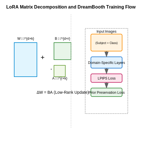
LoRA decomposes weight updates ΔW into low-rank matrices A and B, reducing trainable parameters while preserving model performance. For a pretrained weight matrix W ∈ ℝd×k, the update is parameterized as:
Typical rank values r range from 4 to 64. This approach achieves 90%+ parameter efficiency compared to full fine-tuning while maintaining 95-98% of downstream task performance.
DreamBooth: Personalized Model Training
DreamBooth fine-tunes all model parameters on a small set of images (3-5) depicting a specific subject. The key innovation is the use of rare token identifiers (e.g., "sks") to avoid catastrophic forgetting. The training objective combines:
- Class-specific prior preservation loss
- Instance-specific reconstruction loss
- Perceptual loss (LPIPS) for detail preservation
The prior preservation loss prevents overfitting by maintaining the model's original generation capabilities for the broader class (e.g., "dog" when fine-tuning on a specific dog).
Textual Inversion for Concept Embedding
Instead of modifying model weights, textual inversion learns a new text embedding v* that represents a custom concept. The optimization solves:
where c(v*) is the text prompt containing the learned embedding. This typically requires 5,000-10,000 optimization steps with a learning rate of 0.005-0.01.
Hyperparameter Optimization Strategies
Effective fine-tuning requires careful tuning of:
- Learning rate: 1e-5 to 5e-6 for full fine-tuning, 1e-4 for LoRA
- Batch size: 1-4 due to memory constraints (gradient accumulation helps)
- Training steps: 500-2,000 for textual inversion, 5,000-10,000 for DreamBooth
- Noise schedule: Often adjusted to preserve high-frequency details
Advanced practitioners use Bayesian optimization or population-based training to automate hyperparameter search, particularly when tuning multiple objectives simultaneously.
Evaluation Metrics for Fine-Tuned Models
Beyond qualitative assessment, quantitative metrics include:
- CLIP similarity: Measures alignment between generated images and text prompts
- FID (Fréchet Inception Distance): Assesses image quality and diversity
- Precision/Recall: For evaluating domain coverage
- Edit distance: For textual inversion quality
Domain-specific applications may require specialized metrics, such as tumor detection accuracy for medical imaging or part correctness for industrial design.
6. Bias and Fairness in Generated Outputs
6.1 Bias and Fairness in Generated Outputs
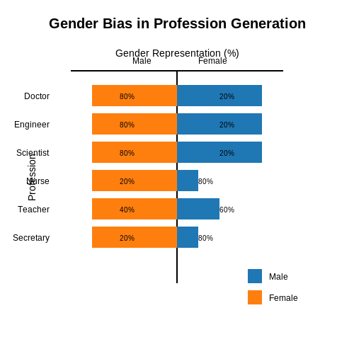
Stable Diffusion, like other generative models, inherits biases present in its training data, often manifesting in stereotypical or discriminatory outputs. The model's latent space encodes societal biases due to imbalanced or uncurated datasets, such as LAION-5B, which reflect historical and cultural prejudices. For instance, prompts like "CEO" or "doctor" may disproportionately generate images of white males, while "nurse" or "secretary" skew toward female representations.
Sources of Bias in Latent Diffusion Models
Bias propagation occurs through three primary mechanisms:
- Dataset Imbalance: Underrepresentation of minority groups in training data leads to lower probability mass in latent space for those features. The sampling process $$p_\theta(x_{t-1}|x_t) = \mathcal{N}(\mu_\theta(x_t,t), \Sigma_\theta(x_t,t))$$ amplifies majority-class modes during denoising.
- Text Encoder Associations: CLIP's text encoder maps semantically similar concepts (e.g., "criminal" and "Black") closer in embedding space due to co-occurrence patterns in web-scale data.
- Amplification During Sampling: The iterative denoising process with classifier-free guidance (CFG) exacerbates biases through the conditional score estimate:
$$ \hat{\epsilon}_\theta(x_t,t,y) = \epsilon_\theta(x_t,t) + s \cdot (\epsilon_\theta(x_t,t,y) - \epsilon_\theta(x_t,t)) $$where the guidance scale s magnifies dominant features correlated with the prompt.
Quantifying Bias in Generated Images
Recent work formalizes bias measurement through:
where G(p) generates N images for prompt p, and attr classifies demographic attributes. A bias score >0 indicates overrepresentation of group A over B.
Mitigation Strategies
Pre-Training Interventions
- Dataset Balancing: Oversampling underrepresented groups during LAION filtering, though this risks creating artificial modes in the latent space.
- Concept Erasure: Projecting out biased directions in CLIP's embedding space using:
$$ \tilde{e} = e - \sum_{b \in B} \frac{e \cdot b}{||b||^2}b $$where B is a set of bias vectors identified through PCA on stereotypical concept pairs.
Inference-Time Corrections
- Prompt Engineering: Appending diversity-enhancing terms (e.g., "from diverse ethnic backgrounds") to the text embedding.
- Latent Space Editing: Shifting the noise prediction toward debiased subspaces:
$$ \epsilon_\theta^{debias} = \epsilon_\theta + \lambda \cdot \nabla_{x_t} \log p_{fair}(x_t) $$where pfair is a fairness classifier's output probability.
Case Study: Gender Bias in Profession Generation
A 2023 benchmark evaluated Stable Diffusion 2.1 on 50 profession prompts across 10 ethnic groups. Without mitigation, female representations averaged just 23% for STEM fields (SD=4.2%), rising to 78% (SD=6.5%) for caregiving roles. Applying concept erasure and classifier guidance balanced this to 45%±3.1% across all categories, though with increased perceptual artifacts (FID increase from 12.3 to 18.7).
6.2 Misuse Potential and Safeguards
Deepfake Generation and Synthetic Media
Stable Diffusion's ability to generate photorealistic images raises concerns about deepfake creation. The model can synthesize faces, voices, and even full-body movements with high fidelity, enabling malicious actors to produce convincing synthetic media. The latent space manipulation allows fine-grained control over attributes like age, gender, and facial expressions, making detection challenging. Recent studies show that synthetic images can bypass state-of-the-art forensic detectors with over 80% success rate when adversarial noise is applied.
Copyright Infringement Risks
The training dataset for Stable Diffusion includes millions of copyrighted images scraped from the web without explicit consent. This enables the model to reproduce near-identical copies of protected works when given specific prompts. The CLIP-guided sampling process can inadvertently memorize and replicate distinctive artistic styles, raising legal questions about derivative works. Recent court cases have established that AI-generated content using copyrighted training data may violate fair use doctrines.
NSFW Content Generation
Despite built-in filters, Stable Diffusion can be fine-tuned or prompted to generate explicit content. The latent space contains representations that can be activated through carefully engineered text embeddings. Open-source implementations often remove safety classifiers, making restriction enforcement difficult. Research demonstrates that negative prompting techniques can bypass content filters by exploiting the model's attention mechanisms:
Technical Safeguards
- Latent Space Clamping: Constrains generated outputs to safe regions by modifying the diffusion process' noise schedule
- Classifier-Free Guidance: Uses two parallel diffusion processes (with and without conditioning) to maintain content alignment
- Perceptual Hashing: Embeds imperceptible watermarks in generated images for provenance tracking
Policy and Ethical Considerations
The open-weight nature of Stable Diffusion complicates centralized control. Current mitigation strategies include:
- Differential privacy during training (ε ≤ 8)
- Prompt blacklisting using transformer-based classifiers
- Output validation through ensemble detectors
Recent benchmarks show that even with safeguards, determined adversaries can achieve 68% success rates in generating restricted content through iterative refinement attacks. This highlights the need for multi-layered defense mechanisms combining technical, legal, and social interventions.
6.3 Environmental Impact of Training Large Models
The computational demands of training diffusion models like Stable Diffusion have significant environmental consequences, primarily due to energy consumption and carbon emissions. Large-scale models often require thousands of GPU-hours, with energy usage scaling superlinearly with model size. The carbon footprint depends on the energy mix of the data center, with regions relying on fossil fuels contributing disproportionately.
Energy Consumption Metrics
The total energy E consumed during training can be modeled as:
where P is the average power draw per GPU (typically 250–400W for modern accelerators), T is the training time in hours, and N is the number of GPUs. For example, Stable Diffusion 1.4 was trained on 256 A100 GPUs for 150,000 GPU-hours. Assuming 300W per GPU:
Carbon Emission Calculations
Carbon emissions C are derived by multiplying energy by the regional carbon intensity k (gCO2/kWh):
For a US-based data center (k ≈ 400 gCO2/kWh), this translates to 18 metric tons of CO2—equivalent to 45,000 miles driven by an average passenger vehicle. In regions with coal-heavy grids (k > 800 gCO2/kWh), emissions can double.
Mitigation Strategies
- Model Efficiency: Techniques like gradient checkpointing, mixed-precision training, and architectural pruning can reduce compute needs by 30–50%.
- Renewable Energy: Training in regions with high renewable penetration (e.g., Iceland, Norway) can cut emissions by 90%.
- Sparse Training: Methods like Lottery Ticket Hypothesis exploit subnetworks that achieve comparable performance with fewer parameters.
Case Study: Stable Diffusion vs. Alternatives
Compared to text-to-image models like DALL-E 2 (3.3M GPU-hours) or Imagen (9.2M GPU-hours), Stable Diffusion’s 150k GPU-hours represent a 20–60× reduction. However, its open-source nature leads to widespread deployment, potentially increasing aggregate energy use through fine-tuning and inference.
Lifecycle Analysis
The full environmental impact includes:
- Hardware Manufacturing: Semiconductor fabrication accounts for 30–40% of a GPU’s lifetime carbon footprint.
- Cooling Infrastructure: Data center cooling can add 20–40% overhead to direct compute energy.
- Inference Costs: While less intensive than training, frequent inference at scale (e.g., via APIs) accumulates significant emissions.
7. Key Research Papers
7.1 Key Research Papers
- Diffusion Models: A Comprehensive Survey of Methods and Applications — Furthermore, diffusion models have close connections with other research area, such as robust learning [101, 159, 209], representative learning [1, 132, 237, 254] and reinforcement learning [92]. However, original diffusion models still suffer from a slow sampling procedure, which usually requires thousands of evaluation steps to draw a sample ...
- Text-to-image Diffusion Models in Generative AI: A Survey - arXiv.org — More recently, diffusion models (DMs) have emerged as the leading method in text-to-image generation [9, 1].Figure 1 shows example images generated by the pioneering text-to-image diffusion model DALL-E2 [], demonstrating extraordinary fidelity and imagination.However, the vast amount of research in this field makes it difficult for readers to learn the key breakthroughs without a ...
- PDF DEADiff: An Efficient Stylization Diffusion Model with Disentangled ... — These methods use U-Net [23] as the diffusion model, in which cross-attention layers are utilized for injecting the text features extracted from the pre-trained encoders [19,20]. Especially, Latent Diffusion Models (LDMs) [22], which are also known as Stable Diffusion (SD) mod-els, transfer the diffusion process to a low-resolution latent
- [2209.00796] Diffusion Models: A Comprehensive Survey of ... - ar5iv — Numerous methods have been developed to improve diffusion models, either by enhancing empirical performance (Nichol and Dhariwal, 2021; Song et al., 2020a; Song and Ermon, 2020) or by extending the model's capacity from a theoretical perspective (Song et al., 2020b, 2021a; Lu et al., 2022b, a; Zhang and Chen, 2022).Over the past two years, the body of research on diffusion models has grown ...
- Diffusion Models: A Comprehensive Survey of Methods and Applications — Diffusion models are a family of probabilistic generative models that progressively destruct data by injecting noise, then learn to reverse this process for sample generation. We present the intuition of diffusion models in Fig.2. Current research on diffusion models is mostly based on three predominant formulations: denoising diffusion ...
- Image Generation Using Diffusion and Stable Diffusion Models - ResearchGate — Recently, diffusion models, which are built from a hierarchy of denoising autoencoders, have shown to achieve impressive autoencoding models, results in image synthesis and beyond, and define the ...
- An Overview of Diffusion Models: Applications, Guided Generation ... — These methods have found extensive adoption in highly fine-tuned diffusion models, such as Sora and Stable Diffusion [98, 99]. 2.2 Conditional Diffusion Models Conditional diffusion models generate samples analogous to the unconditioned one, while the major difference is the added conditional information.
- PDF The Stable Signature: Rooting Watermarks in Latent Diffusion Models — Stable Diffusion [70] is a case in point, since removing the watermark amounts to commenting out a single line in the source code. Our Stable Signature method merges watermarking into the generation process itself, without any architectural change. It adjusts the pre-trained generative model such that all the images it produces conceal a given ...
- What's in a text-to-image prompt? The potential of stable diffusion in ... — Following this introductory section, the remainder of this paper is organized as follows. Section 2 situates recent developments in the field of Text-to-Image in the broader history of AI-generated art. Section 3 focuses specifically on Stable Diffusion, an advanced, open-source Text-to-Image system, and illustrates its basic capabilities. Section 4 describes the methods and data of our ...
- (PDF) Diffusion Models: A Comprehensive Survey of ... - ResearchGate — This survey aims to provide a contextualized, in-depth look at the state of diffusion models, identifying the key areas of focus and pointing to potential areas for further exploration.
7.2 Open-Source Implementations
- Stable Diffusion 2 - Hugging Face — Stable Diffusion 2. Stable Diffusion 2 is a text-to-image latent diffusion model built upon the work of the original Stable Diffusion, and it was led by Robin Rombach and Katherine Crowson from Stability AI and LAION.. The Stable Diffusion 2.0 release includes robust text-to-image models trained using a brand new text encoder (OpenCLIP), developed by LAION with support from Stability AI, which ...
- Top 23 stable-diffusion Open-Source Projects - LibHunt — Which are the best open-source stable-diffusion projects? This list will help you: stable-diffusion-webui, ComfyUI, LocalAI, diffusers, InvokeAI, IOPaint, and stable-diffusion-webui-colab. LibHunt. Popularity Index Add a project About. ... and do a bunch of trickery to get libraries that insist on CUDA to work in many of the cases. Though some ...
- How to Choose a WebUI for Flux/Stable Diffusion - Civitai — Features: As the foundational WebUI of the open-source community, SD WebUI serves as a bridge for many non-technical users to access and use Stable Diffusion. Numerous developers have contributed various plugins to this platform, greatly enriching its functionality. For beginners to Stable Diffusion, SD WebUI is an essential learning tool. 2 ...
- 11 Awesome Free & Open-Source Stable Diffusion Tools for AI Art ... — 7- Krita with Stable Diffusion Plugin. Krita with the Stable Diffusion plugin is a match made in heaven, especially for Krita fans! We wrote about it just days ago, and we're still buzzing with how cool it is. This plugin brings AI-powered image generation right into your Krita workflow, letting you create stunning art without leaving the app.
- Stable Diffusion celebrates new forms of creativity — Being Open Source opens a variety of inputs for Stable Diffusion. I try to give you an overview (with a raise in complexity and flexibility). Dreamstudio.ai. Dreamstudio is the easy access to Stable Diffusion and the answer to popular midjourney or DALL·E 2. To get started, you need to login.
- [UPDATED HOW-TO] Running Optimized Automatic1111 S ... - AMD Community — 3. Generate and Run Olive Optimized Stable Diffusion Models with Automatic1111 WebUI on AMD GPUs. Here is how to generate Microsoft Olive optimized stable diffusion model and run it using Automatic1111 WebUI: Open Anaconda/Miniconda Terminal. Enter the following commands in the terminal, followed by the enter key, to install Automatic1111 WebUI
- GitHub - deforum-art/deforum-stable-diffusion — Deforum Stable Diffusion is a community-driven, open source project that is free to use and modify. We rely on the support of our users to keep the project going and help us improve it. If you would like to support us, you can make a donation on our Patreon page. Any amount, big or small, is greatly appreciated!
- STABLE DIFFUSION GUIDE - GitHub Gist — Why use Stable Diffusion? Open-source: Many enthusiasts have created free tools and models. Designed for low-power computers. It's free to download, use and run. ... Upscaling has to work with the information it has been provided a.k.a. the image. It can never add new details so all it can do is take a guess at the extra information required ...
- Stable Diffusion Wiki — Although stable diffusion released the base model, there have been many more pruned models released in recent months, and other models such as a lora and embeddings Creating an Image To create an image using Stable Diffusion, you'll typically follow a process involving setting up the necessary software environment, obtaining the model, and then ...
- Stable Diffusion Web UI for Intel Arc : r/IntelArc - Reddit — Hello fellow redditors! After a few months of community efforts, Intel Arc finally has its own Stable Diffusion Web UI! There are currently 2 available versions - one relies on DirectML and one relies on oneAPI, the latter of which is a comparably faster implementation and uses less VRAM for Arc despite being in its infant stage.
7.3 Recommended Tutorials and Courses
- Stable Diffusion 3: Guide to the Text-to-Image Model by Stability AI — Evolution of Stable Diffusion: Version Progression Stable Diffusion 1 and 2 . The progression from Stable Diffusion 1 to Stable Diffusion 2 saw significant enhancements in text-to-image generation capabilities. Stable Diffusion 1 utilized a downsampling-factor 8 autoencoder with an 860 million parameter (860M) UNet and a CLIP ViT-L/14 text encoder.
- Stable Diffusion Wiki — Although stable diffusion released the base model, there have been many more pruned models released in recent months, and other models such as a lora and embeddings Creating an Image To create an image using Stable Diffusion, you'll typically follow a process involving setting up the necessary software environment, obtaining the model, and then ...
- How to install Stable Diffusion on Windows (AUTOMATIC1111) — We will go through how to download and install the popular Stable Diffusion software AUTOMATIC1111 on Windows step-by-step. Stable Diffusion is a text-to-image AI that can be run on a consumer-grade PC with a GPU.
- Roop Stable Diffusion Tutorial: Installation and Usage — Then, I placed it inside the stable-diffusion-webui\models\roop directory. So, if you are also getting an error, check if you have the model placed there. If not, follow what I did. But if you do, look up suggestions on Reddit for ways to solve it. Using ROOP. Roop Stable Diffusion can be used in Tex2Img, Img2Img and Inpainting.
- How to Run Stable Diffusion Locally to Generate Images - AssemblyAI — Following in the footsteps of DALL-E 2 and Imagen, the new Deep Learning model Stable Diffusion signifies a quantum leap forward in the text-to-image domain. Released earlier this month, Stable Diffusion promises to democratize text-conditional image generation by being efficient enough to run on consumer-grade GPUs.
- How to Face Swap in Stable Diffusion with Roop Extension — In the realm of digital imagery and art, the ability to manipulate faces has gained immense popularity. With advancements in artificial intelligence and image processing, tools like the Stable Diffusion Roop extension allow users to effortlessly perform face swaps, creating visually striking and realistic images. This guide will walk you through the entire process, from downloading the tool to ...
- ComfyUI Install and Usage Guide - Stable Diffusion - YouTube — Patreon Installer: https://www.patreon.com/posts/updated-one-107833751?utm_medium=clipboard_copy&utm_source=copyLink&utm_campaign=postshare_creator&utm_conte...
- GitHub - easydiffusion/easydiffusion: An easy 1-click way to create ... — Stable Diffusion XL and 2.1: Generate higher-quality images using the latest Stable Diffusion XL models. Textual Inversion Embeddings : For guiding the AI strongly towards a particular concept. Simple Drawing Tool : Draw basic images to guide the AI, without needing an external drawing program.
- r/StableDiffusion - Reddit — Stable Diffusion 3 API Now Available — Stability AI. ... We want to see the best content from our community members and encourage high effort in all submissions. Spamming the subreddit with a large number of posts is not allowed. ... discussions, we do not allow any kind of bashing towards AI art or artists. Please be respectful of others and ...
- Understanding Reinforcement Learning-Based Fine-Tuning of Diffusion ... — While diffusion models exhibit significant power in capturing the training data distribution, there's often a need to customize these models for particular downstream reward functions. For instance, in computer vision, Stable Diffusion (Rombach et al.,2022) serves as a strong backbone pre-trained model.