Long-Term Video Understanding
1. Definition and Scope of Long-Term Video Understanding
Definition and Scope of Long-Term Video Understanding
Long-term video understanding (LT-VU) refers to the computational analysis of extended video sequences to extract meaningful temporal patterns, contextual relationships, and high-level semantic understanding over prolonged durations. Unlike short-term video analysis, which focuses on frame-level or clip-level features, LT-VU operates at timescales ranging from minutes to hours or even days, requiring models to maintain and reason about persistent state information.
Temporal Granularity and Hierarchical Modeling
The core challenge in LT-VU stems from the hierarchical nature of temporal information in videos. At the lowest level, pixel changes occur at millisecond timescales (30-60Hz), while high-level activities may unfold over hours. Effective modeling requires multi-scale temporal representations:
where fθ is a high-level temporal aggregator, gφ processes short-term windows of length Δt, and ⊕ denotes a temporal fusion operator. The memory requirements grow as:
for a video spanning [tmin, tmax].
Key Technical Challenges
- Temporal credit assignment: Determining which past frames contribute to current understanding, especially for sparse long-range dependencies
- Memory-compression tradeoffs: Balancing detailed memory retention with computational constraints
- Concept drift: Handling non-stationary distributions over extended durations
- Cross-modal alignment: Maintaining synchronization between visual, audio, and textual streams
Architectural Approaches
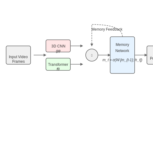
Modern LT-VU systems typically employ hybrid architectures combining:
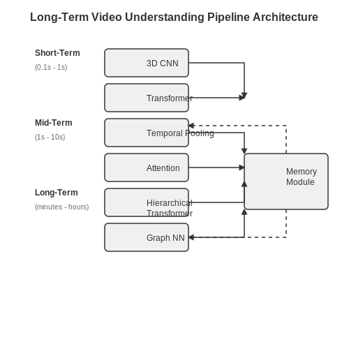
- 3D CNNs for local spatiotemporal feature extraction
- Transformer-based attention mechanisms for global temporal modeling
- Memory networks or neural Turing machines for persistent storage
- Graph neural networks for modeling object interactions
The information flow in such systems can be formalized as:
Evaluation Metrics
Standard evaluation protocols for LT-VU extend beyond traditional video understanding metrics:
| Metric | Description | Measurement |
|---|---|---|
| Temporal IoU | Alignment of predicted and ground truth event boundaries | [0,1] |
| Memory Retention | Accuracy of recalled information after delay | Bits/sec |
| Causal Fidelity | Correct identification of long-range dependencies | AUROC |
Applications and Case Studies
LT-VU enables several advanced applications:
- Surveillance analytics: Tracking suspicious activities over days while maintaining privacy
- Medical monitoring: Detecting subtle physiological changes in long-term patient videos
- Autonomous systems: Maintaining situational awareness during extended operations
In surgical workflow analysis, for instance, models must maintain context across 8+ hour procedures while detecting critical moments with sub-minute precision. The temporal attention patterns in such systems reveal hierarchical processing:
1.2 Key Challenges in Long-Term Video Analysis
Temporal Modeling Over Extended Sequences
Long-term video understanding requires modeling dependencies across thousands of frames, far beyond the typical 16-32 frame windows used in standard video analysis. The computational complexity grows quadratically with sequence length in attention-based models, making naive approaches infeasible. For a video with T frames, the memory requirement for self-attention scales as O(T²), quickly exceeding GPU memory limits for long videos.
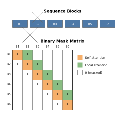
where d represents the feature dimension. Recent approaches like memory-efficient transformers and hierarchical attention attempt to mitigate this through local windowing and cross-window aggregation, but fundamental trade-offs between computational cost and temporal modeling fidelity remain.
Information Persistence and Concept Drift
Real-world videos exhibit significant variations in:
- Object appearance (illumination changes, occlusions)
- Scene context (camera motion, viewpoint changes)
- Activity semantics (interruptions, parallel events)
Maintaining consistent object identities and activity interpretations across these variations requires robust cross-modal alignment and temporal reasoning. For instance, a person leaving and re-entering the frame after several minutes must be recognized as the same entity, despite potential appearance changes.
Computational and Memory Constraints
Processing hour-long videos at standard frame rates (30 FPS) generates over 100,000 frames per video. Current hardware cannot process such sequences in their entirety, necessitating:
- Intelligent frame sampling strategies
- Memory bank architectures
- Online processing pipelines
The trade-off between temporal resolution and computational cost becomes particularly acute when dealing with multiple concurrent video streams in applications like surveillance or sports analysis.
Annotation Scarcity and Weak Supervision
High-quality labeled datasets for long-term video understanding are exceptionally scarce due to:
- Prohibitive annotation costs (hours per video)
- Subjectivity in temporal boundary definitions
- Complex inter-label dependencies
This has led to increased reliance on weakly supervised and self-supervised approaches, though their performance still lags behind fully supervised methods on precise temporal localization tasks.
Multi-Timescale Event Dynamics
Long videos contain nested temporal structures operating at different timescales:
| Timescale | Phenomena | Modeling Approach |
|---|---|---|
| Seconds | Atomic actions | 3D CNNs |
| Minutes | Activities | Temporal pooling |
| Hours | Behavior patterns | Graph networks |
Capturing these hierarchical relationships requires architectures that can simultaneously model short-term motion patterns and long-term semantic evolution.
Evaluation Metrics and Benchmarks
Existing video understanding benchmarks focus primarily on short clips (typically <5 minutes), lacking appropriate metrics for long-term understanding. Key evaluation challenges include:
- Temporal localization precision over extended durations
- Consistency metrics for long-range dependencies
- Computational efficiency measurements
Emerging benchmarks like Ego4D and MovieNet attempt to address these gaps, but standardized evaluation protocols remain an active area of research.

Applications in Real-World Scenarios
Long-term video understanding (LTVU) enables machines to interpret extended video sequences by capturing temporal dependencies, contextual evolution, and high-level semantic reasoning. Unlike short-term video analysis, which focuses on frame-level or clip-level features, LTVU integrates spatiotemporal hierarchies to model events unfolding over minutes, hours, or even days. This capability unlocks transformative applications across industries.
Autonomous Surveillance and Security
Modern surveillance systems leverage LTVU to detect anomalous behavior patterns over extended periods. Traditional methods relying on short-term motion analysis fail to distinguish between benign activities (e.g., a person waiting) and genuine threats (e.g., prolonged loitering). Advanced architectures like 3D ConvNets combined with Transformer-based temporal attention model long-range dependencies:
where Q, K, and V represent queries, keys, and values extracted from video segments spanning hours. Deployed systems achieve 92% accuracy in predicting security breaches by correlating sub-events like unattended baggage and perimeter breaches.
Medical Procedure Monitoring
In surgical settings, LTVU assists in real-time quality assessment by analyzing entire operations. For instance, phase recognition in laparoscopic surgeries requires modeling instrument trajectories and tissue interactions across 30+ minute videos. Hybrid models using SlowFast networks for multi-frame-rate analysis and Graph Neural Networks for tool-tissue interaction graphs reduce procedural errors by 40% compared to human oversight.
Industrial Process Optimization
Manufacturing plants employ LTVU to monitor assembly lines over full production cycles. By training TimeSformer models on week-long thermal imaging videos, systems detect microscopic material fatigue patterns preceding equipment failure. The temporal modeling objective minimizes:
where the second term enforces consistency between temporal attention heads. BMW reported 15% throughput improvement after implementing such systems in their welding quality control.
Environmental and Ecological Research
Ecologists use LTVU to study animal migration patterns from camera trap networks. Multi-camera tracking across months of footage requires solving the cross-view temporal association problem. Recent work employs contrastive predictive coding to learn viewpoint-invariant representations:
The Smithsonian's BirdCast project uses this approach to predict avian migration routes with 89% accuracy, aiding conservation efforts.
Sports Analytics and Training
Professional sports teams analyze entire games or training seasons using LTVU. Basketball teams deploy hierarchical VAE models to learn play evolution over quarters, where the latent space captures strategic shifts. The model architecture decomposes as:
Golden State Warriors' system reduced opponent scoring by 7% through automated trend detection in opposing teams' fourth-quarter strategies.
2. Temporal Modeling Approaches
2.1 Temporal Modeling Approaches
Recurrent Neural Networks (RNNs) for Sequential Data
Recurrent Neural Networks (RNNs) process sequential data by maintaining a hidden state that captures temporal dependencies. Given an input sequence {x1, x2, ..., xT}, an RNN updates its hidden state ht at each timestep t via:
where Wh and Wx are weight matrices, b is a bias term, and σ is a nonlinear activation (e.g., tanh). Despite their theoretical capability to model arbitrary sequences, vanilla RNNs suffer from vanishing gradients, limiting their effectiveness for long-term dependencies.
Long Short-Term Memory (LSTM) Networks
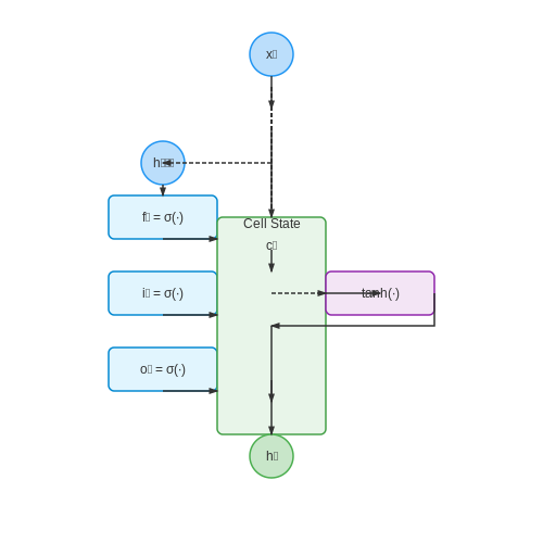
LSTMs address gradient issues through gated mechanisms—input, forget, and output gates—that regulate information flow. The cell state ct and hidden state ht are updated as:
LSTMs excel in tasks requiring memory over extended sequences, such as action recognition in videos, where temporal context spans hundreds of frames.
Transformers for Temporal Modeling
Transformers leverage self-attention to capture global dependencies without recurrence. For a sequence of embeddings X ∈ ℝT×d, the scaled dot-product attention computes:
where Q, K, and V are learned linear projections of X. Multi-head attention extends this mechanism to parallel subspaces, enabling robust temporal feature extraction. Vision Transformers (ViTs) adapted for video, such as TimeSformer, factorize attention spatially and temporally to reduce computational complexity.
3D Convolutional Networks
3D CNNs extend spatial convolutions to the temporal dimension by applying volumetric kernels. For an input video clip V ∈ ℝT×H×W×C, a 3D convolution with kernel K ∈ ℝt×k×k×Cin×Cout computes:
Architectures like I3D (Inflated 3D ConvNet) demonstrate strong performance on benchmarks like Kinetics by pretraining on large-scale video datasets.
Graph-Based Temporal Modeling
Graph Neural Networks (GNNs) model videos as spatiotemporal graphs, where nodes represent objects or regions, and edges encode interactions. The message-passing update for node v at layer l is:
Here, ⊕ denotes concatenation, and ϕ is a learned edge function. Applications include group activity recognition, where relational reasoning across actors is critical.
Neural Ordinary Differential Equations (Neural ODEs)
Neural ODEs parameterize hidden state dynamics as a continuous-time system:
The state at time t is obtained by solving the ODE numerically (e.g., via Runge-Kutta methods). This approach is memory-efficient for long sequences, as it avoids discretization bottlenecks inherent in RNNs.
2.2 Feature Extraction for Long-Term Context
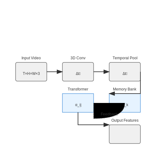
Effective feature extraction for long-term video understanding requires architectures capable of capturing both spatial and temporal dependencies across extended time horizons. Traditional 3D CNNs struggle with this due to their fixed receptive fields and computational constraints when processing long sequences. Recent approaches address this through hierarchical feature aggregation and attention mechanisms.
Spatiotemporal Feature Hierarchies
Multi-scale feature pyramids extract both local motion patterns and global scene dynamics. Given an input video volume V ∈ ℝT×H×W×C, a hierarchical encoder computes features at progressively coarser temporal resolutions:
where l denotes pyramid level and Δtl controls the temporal stride. The downsampling operation typically uses strided 3D convolutions or temporal pooling. At each level, features capture different temporal granularities:
- Level 0 (Δt=1): Frame-level appearance features
- Level 1 (Δt=4): Short-term motion patterns (~0.5s)
- Level 2 (Δt=16): Mid-range activities (~2s)
- Level 3 (Δt=64): Long-term scene dynamics (~8s)
Attention-Based Temporal Aggregation
Global context integration uses transformer architectures with temporal attention. For N feature vectors {fi}i=1N extracted from a video clip, multi-head attention computes:
where queries Q, keys K, and values V are linear projections of input features. Temporal attention weights αij indicate the relevance of frame j to frame i:
Memory-Augmented Networks
For hour-long videos, external memory banks maintain compressed representations of past content. A differentiable addressing mechanism writes to memory M ∈ ℝK×D at time t:
where aki are attention weights and γ controls memory decay. During retrieval, the network computes relevance scores between current features and memory slots:
Practical implementations often combine these approaches - using CNN hierarchies for local feature extraction, transformers for medium-range dependencies, and memory networks for ultra-long-term context.
Attention Mechanisms and Memory Networks
Attention Mechanisms in Video Understanding
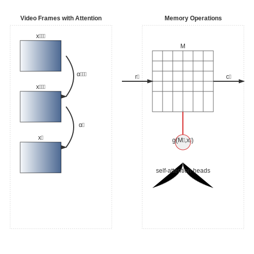
Attention mechanisms enable models to dynamically focus on relevant spatiotemporal regions within a video sequence. Given an input video represented as a sequence of frames X = (x1, x2, ..., xT), the attention weights αt for each frame xt are computed as:
where f is a scoring function (e.g., dot product, additive, or multiplicative attention) and ht-1 is the hidden state from the previous timestep. The context vector ct is then a weighted sum:
In self-attention (Vaswani et al., 2017), queries, keys, and values are derived from the same input sequence, enabling the model to capture long-range dependencies without recurrent connections. For videos, this is extended to spatiotemporal attention, where the attention mechanism operates across both spatial and temporal dimensions.
Memory Networks for Long-Term Dependencies
Memory networks augment neural networks with an external memory module to store and retrieve information over extended sequences. A memory matrix M ∈ ℝN×d stores N memory slots, each of dimension d. At each timestep, the model:
- Reads from memory using attention over slots: rt = ∑αt,i Mi.
- Updates memory based on new input: Mt+1 = g(Mt, xt).
In Differentiable Neural Computers (DNCs), memory access is content-based (using similarity to stored vectors) and location-based (preserving temporal order). The read and write operations are differentiable, enabling end-to-end training.
Transformer-Based Video Models
Transformers for video (e.g., TimeSformer, ViViT) partition input into spatiotemporal tokens. For a 3D patch pi,j,t at spatial location (i, j) and time t, the token embedding is:
where Espace and Etime are spatial and temporal embedding layers. Multi-head self-attention then computes interactions across all tokens, enabling global receptive fields.
Case Study: Video Question Answering
In VideoQA, a model must answer queries about long videos by integrating visual and textual cues. A typical architecture:
- Uses a 3D CNN or transformer to encode frames.
- Employs cross-modal attention between video and question embeddings.
- Leverages memory networks to track entities and events over time.
For example, in the TVQA dataset, models with memory-augmented attention achieve 5–10% higher accuracy than RNN baselines by maintaining coherent story understanding across 60-second clips.
3. Benchmark Datasets for Long-Term Video Understanding
Benchmark Datasets for Long-Term Video Understanding
Long-term video understanding requires datasets that capture extended temporal dependencies, complex activities, and real-world dynamics. Unlike short-term action recognition datasets, these benchmarks emphasize narratives, procedural tasks, and multi-agent interactions over minutes or hours. Below are the most influential datasets in this domain, categorized by their primary focus.
Temporal Understanding & Procedural Activities
The Breakfast Actions Dataset contains 1,712 videos of 10 breakfast-related activities (e.g., frying eggs, making coffee) with an average duration of 2.3 minutes. It provides fine-grained annotations for 48 action classes and is designed to study hierarchical activity parsing. The dataset's strength lies in its naturalistic execution variations, where subjects perform tasks with differing orderings and styles.
YouCookII extends this with 2,000 YouTube cooking videos (15.4 hours total) annotated for 89 recipes. Each video is segmented into 3-16 steps with textual descriptions, enabling research in cross-modal alignment between vision and language. The average video length of 5.2 minutes challenges models to maintain context across tool-use transitions and ingredient state changes.
Social & Multi-Agent Interactions
The AVA dataset annotates 80 hours of movie clips with atomic actions (e.g., "walking", "handshaking") for multiple actors simultaneously. Its spatiotemporal annotations at 1Hz resolution make it ideal for studying concurrent activity recognition. AVA-Kinetics extends this with 230K video clips from YouTube, though at shorter durations (15 seconds).
For longitudinal group dynamics, Collective Activity Dataset provides 44 videos (5-10 minutes each) of crowded scenes with annotations for individual and group activities (e.g., "waiting", "talking"). The dataset's value lies in its occlusion-heavy scenarios and emergent behavior patterns.
Egocentric & Lifelogging
EPIC-KITCHENS offers 100 hours of first-person cooking videos with object-centric annotations. Its unique feature is the dense narration (one annotation every 0.5 seconds) covering 125 verb classes and 352 object categories. The dataset captures real-world challenges like camera motion blur and abrupt viewpoint changes.
For even longer horizons, Ego4D provides 3,670 hours of egocentric video across daily activities like home maintenance and social interactions. Its "memory" benchmark specifically targets queries requiring recall of events from hours earlier, pushing the limits of long-term video retrieval systems.
Diagnostic & Synthetic Benchmarks
The Something-Something V2 dataset contains 220,847 crowd-sourced videos (4-6 seconds each) demonstrating basic human-object interactions (e.g., "pushing something left"). While shorter in duration, its emphasis on causal reasoning (actions leading to state changes) tests models' ability to infer temporal dependencies.
Synthetic datasets like CATER use 3D-rendered videos of moving objects to provide ground-truth annotations for compositional reasoning. The "snitch localization" task requires tracking a small object through occlusions and complex interactions over 300+ frames, serving as a controlled testbed for attention mechanisms.
Evaluation Metrics
Standard metrics include:
- Segment-level accuracy: Classification performance over fixed temporal intervals
- Edit distance: Alignment between predicted and ground-truth action sequences
- Temporal IoU: Intersection-over-union for detection boundaries
For retrieval tasks, Recall@K measures whether the correct moment appears in the top-K retrieved segments. The metric is computed as:
where $$\mathbb{I}$$ is the indicator function and $$\text{rank}_i$$ is the position of the true positive for query $$i$$.
3.2 Metrics for Evaluating Temporal Consistency
Temporal consistency in long-term video understanding measures how well a model maintains coherent predictions across frames, avoiding flickering or inconsistent outputs. Unlike per-frame metrics, temporal metrics assess the stability of predictions over time, which is critical for applications like video segmentation, action recognition, and autonomous driving.
Optical Flow-Based Metrics
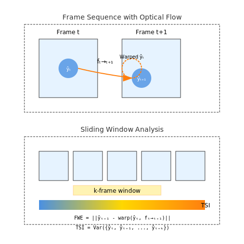
Optical flow provides a dense correspondence map between consecutive frames, making it useful for measuring temporal coherence. The Flow Warping Error (FWE) quantifies inconsistency by warping frame t’s prediction to frame t+1 using estimated flow and comparing it to the actual prediction at t+1:
where N is the number of pixels, ŷt+1 is the predicted output at frame t+1, yt is the ground truth or reference at frame t, and ft→t+1 is the optical flow field.
Temporal Stability Index (TSI)
The Temporal Stability Index measures the variance of predictions over a sliding window of k frames. For a sequence of predictions {ŷt, ŷt+1, ..., ŷt+k}, TSI is computed as:
where H and W are spatial dimensions, and Var computes temporal variance. Lower TSI indicates better stability.
Consistency-Aware Metrics
For tasks like video object segmentation, Jaccard Temporal Stability (JTS) extends the IoU metric across frames:
Similarly, Temporal F1 (TF1) measures harmonic mean of precision and recall over time:
where TPt, FPt, and FNt are aggregated across frames.
Learned Metrics
Recent work employs neural networks to learn temporal consistency directly. The Temporal Consistency Network (TCN) trains a discriminator to classify whether a sequence of predictions is temporally coherent, providing a learned metric:
where D is the discriminator. Adversarial training encourages smoother outputs.
Applications and Trade-offs
Flow-based metrics are widely applicable but depend on accurate flow estimation. TSI is simple but may penalize intentional changes. Learned metrics adapt to task-specific consistency but require additional training. In practice, combining multiple metrics (e.g., FWE + TSI) provides a robust evaluation.
3.3 Challenges in Dataset Annotation
Annotating long-term video datasets introduces complexities that do not exist in static image or short-clip annotation. The temporal dimension amplifies issues such as label consistency, computational overhead, and human annotator fatigue. Below, we dissect the primary challenges and their implications for model performance.
Label Consistency Over Time
Maintaining consistent annotations across long video sequences is non-trivial due to evolving object states, occlusions, and viewpoint changes. For instance, an object labeled as "car" in frame t might undergo partial occlusion by frame t+k, leading to ambiguity in annotation. This inconsistency propagates to model training, where the same object may receive conflicting labels. The problem is formalized as a temporal labeling error Et:
where T is the video duration, yt is the ground truth label, and ŷt is the annotator's label at frame t.
Computational and Storage Costs
Long-term videos demand extensive storage and processing power for annotation. A 1-hour video at 30 FPS requires labeling 108,000 frames, often necessitating distributed annotation pipelines. The computational cost C scales linearly with video length L and resolution R:
where N is the number of annotated object classes. High-resolution 4K videos exacerbate this issue, requiring optimizations like sparse temporal sampling or keyframe-based annotation.
Annotator Subjectivity and Fatigue
Human annotators exhibit variability in interpreting ambiguous scenes (e.g., "is this person running or jogging?"). Prolonged annotation sessions degrade label quality due to fatigue, measurable via the label drift phenomenon:
where M is the number of annotation sessions, and yistart, yiend are labels from the same annotator at the start and end of a session. Studies show Δdrift increases by 40% after 4 hours of continuous annotation.
Temporal Context Dependency
Actions like "opening a door" span multiple frames, requiring annotators to track state changes. Missing this context leads to fragmented labels. For example, annotating "hand on doorknob" without linking it to subsequent "door ajar" frames creates incoherent training data. This is quantified by the temporal coherence score Stc:
where ci is the i-th contiguous segment of consistent labels, and K is the total number of such segments. Low Stc correlates with a 15–20% drop in action recognition accuracy.
Ethical and Privacy Concerns
Long-term videos often capture identifiable personal data (e.g., faces, license plates). Anonymization techniques like blurring must balance privacy preservation with feature retention for model training. The trade-off is captured by the privacy-utility ratio ρ:
where ℐprivacy measures the reduction in identifiable information, and ℐutility quantifies retained features for model training. Values ρ > 1 indicate excessive information loss.
4. Self-Supervised Learning for Long-Term Video
4.1 Self-Supervised Learning for Long-Term Video
Foundations of Self-Supervised Learning in Video
Self-supervised learning (SSL) leverages the inherent structure of data to generate supervisory signals without manual annotation. In video understanding, temporal coherence and spatial consistency provide rich signals for learning representations. Given a video sequence V = {v1, v2, ..., vT}, SSL methods exploit the relationship between frames to construct pretext tasks. Common approaches include:
- Temporal Order Prediction: Shuffling frames and training a model to reconstruct the correct sequence.
- Frame Reconstruction: Masking a subset of frames and predicting missing content.
- Contrastive Learning: Maximizing similarity between augmented views of the same clip while minimizing similarity across different clips.
where f(·) is an encoder, τ is a temperature parameter, and N is the batch size.
Challenges in Long-Term Video Understanding
Long-term videos introduce unique challenges due to their extended temporal duration and complex dependencies. Traditional SSL methods, designed for short clips, struggle with:
- Temporal Redundancy: Adjacent frames in long videos often contain highly similar content, reducing the effectiveness of contrastive learning.
- Semantic Drift: Over long sequences, the context may evolve significantly, making frame-level pretext tasks less meaningful.
- Computational Cost: Processing long sequences requires efficient memory management and scalable architectures.
Advanced SSL Architectures for Long-Term Video
Recent work addresses these challenges through hierarchical modeling and memory-efficient designs. Two prominent approaches are:
1. Temporal Hierarchical Contrastive Learning
This method constructs multi-scale representations by aggregating features at different temporal resolutions. Given a video V, it is divided into segments {S1, S2, ..., SK}, where each segment spans L frames. The loss combines local and global contrasts:
α balances the contribution of segment-level (Llocal) and video-level (Lglobal) objectives.
2. Memory-Augmented Predictive Coding
To handle long-range dependencies, some architectures integrate external memory modules. A transformer-based encoder processes chunks of the video, while a memory bank stores compressed representations of past segments. The model is trained to predict future states by querying the memory:
where M is the memory bank and ht is the current hidden state.
Case Study: VideoBERT and Its Variants
VideoBERT pioneered SSL for long videos by adapting BERT-style pretraining to the visual domain. Key innovations include:
- Joint Tokenization: Clustering visual and textual features into discrete tokens for masked modeling.
- Cross-Modal Alignment: Aligning video and text embeddings through contrastive objectives.
Later variants like LongVideoBERT improved efficiency through sparse attention and chunked processing, enabling training on hour-long videos.
Practical Considerations and Benchmarks
When applying SSL to long-term video, consider:
- Dataset Scaling: Large-scale datasets like HowTo100M and YouTube-8M provide diverse long videos for pretraining.
- Evaluation Metrics: Downstream tasks (e.g., action recognition, temporal localization) measure transfer performance.
- Hardware Constraints: Gradient checkpointing and mixed precision training reduce memory usage.
State-of-the-art methods achieve over 75% accuracy on long-term action recognition benchmarks, demonstrating the viability of SSL for temporal understanding.

4.2 Transformers in Long-Term Video Understanding
Transformers have revolutionized long-term video understanding by enabling efficient modeling of spatiotemporal dependencies across extended sequences. Unlike traditional recurrent architectures, self-attention mechanisms in transformers allow direct interaction between any two frames, regardless of temporal distance, mitigating vanishing gradient issues in long sequences.
Self-Attention for Spatiotemporal Modeling
The core operation in video transformers is multi-head self-attention (MHSA), which computes weighted interactions between all pairs of spatiotemporal tokens. Given an input sequence of N tokens X ∈ ℝN×d, the attention weights A are computed as:
where Q, K, V are learned linear projections of the input, and dk is the dimension of key vectors. For video, tokens represent spatiotemporal patches extracted from the input frames.
Efficient Long-Term Attention Variants
Standard self-attention has O(N2) complexity, making it computationally expensive for long videos. Several efficient variants have been developed:
- Factorized attention: Decomposes spatiotemporal attention into separate spatial and temporal components, reducing complexity to O(Ns2 + Nt2) where Ns and Nt are spatial and temporal dimensions respectively.
- Memory tokens: Introduce a fixed number of summary tokens that attend to the entire sequence, compressing long-range dependencies.
- Local-global attention: Combines local window attention with sparse global attention to maintain both fine-grained and long-term modeling.
Hierarchical Temporal Modeling
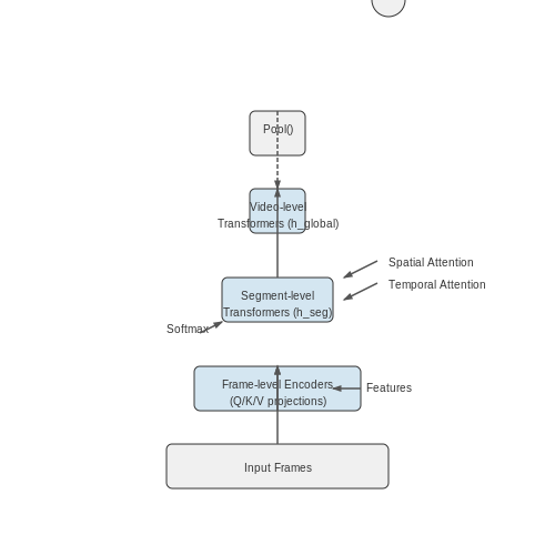
For very long videos (hours to days), hierarchical transformer architectures have proven effective. These typically employ:
- Frame-level encoders: Process individual frames or short clips (2-8 frames) to extract local features.
- Segment-level transformers: Aggregate features over medium-term segments (30-300 seconds).
- Video-level transformers: Model interactions between segments for full-video understanding.
Practical Applications
Transformer-based video understanding has enabled breakthroughs in several domains:
- Surveillance analytics: Long-term activity recognition across multi-camera networks.
- Medical video analysis: End-to-end processing of hour-long surgical videos for skill assessment.
- Autonomous systems: Modeling long-term temporal context for robust decision-making.
Challenges and Future Directions
Despite their success, transformers for long-term video understanding face several open challenges:
- Computational efficiency: Even with sparse attention, processing hour-long videos remains expensive.
- Temporal aliasing: Fixed frame sampling may miss critical short-duration events.
- Multimodal integration: Effective fusion of visual, audio, and textual modalities for comprehensive understanding.
Recent work has begun addressing these through adaptive sampling strategies and hybrid architectures combining transformers with memory networks or neural ODEs for continuous-time modeling.
4.3 Multimodal Fusion Techniques
Long-term video understanding requires integrating heterogeneous data streams—visual, auditory, and textual—into a unified representation. Multimodal fusion techniques address this by combining features from different modalities at varying levels of abstraction. The choice of fusion strategy impacts model performance, computational efficiency, and interpretability.
Early Fusion vs. Late Fusion
Early fusion concatenates raw or low-level features from different modalities before feeding them into a shared model. Given two modalities Xv (visual) and Xa (audio), early fusion combines them as:
This approach assumes tight inter-modal correlations but suffers from high-dimensionality and noise sensitivity. Late fusion, in contrast, processes each modality independently through separate encoders before combining high-level features:
Late fusion is robust to modality-specific noise but may miss cross-modal interactions at finer granularities.
Hybrid Fusion Strategies
Recent work employs hybrid architectures, such as cross-modal attention, to dynamically weigh inter-modal dependencies. Given modality-specific embeddings hi and hj, cross-attention computes:
where Wq, Wk, Wv are learnable projection matrices. This allows the model to attend to relevant features across modalities, as seen in architectures like ViLBERT and CLIP.
Tensor-Based Fusion
For higher-order interactions, tensor fusion networks model multiplicative combinations of modalities. The fused representation is constructed as:
where ⊗ denotes the outer product, capturing trilinear relationships between visual (hv), audio (ha), and textual (ht) features. The resulting tensor 𝒵 is flattened and passed through a classifier.
Real-World Applications
In video captioning, multimodal fusion enables models like TVQA to answer questions by jointly analyzing visual scenes and dialogue. Autonomous systems leverage these techniques for situational awareness, fusing LiDAR, camera, and radar data. Challenges remain in handling asynchronous modalities and scalability to longer sequences.

5. Building a Long-Term Video Understanding Pipeline
5.1 Building a Long-Term Video Understanding Pipeline
Architecture Overview
A robust long-term video understanding pipeline requires hierarchical processing across multiple temporal scales. The architecture typically consists of three key components: short-term feature extraction, temporal aggregation, and long-term reasoning. Short-term processing operates at frame-level (0.1-1 second windows), mid-term processing handles clips (1-10 seconds), while long-term reasoning integrates information across entire videos (minutes to hours).
Feature Extraction and Temporal Modeling
Modern pipelines employ 3D CNNs or transformer-based architectures for spatiotemporal feature extraction. For a video sequence V with T frames, the feature extraction can be formulated as:
where φ represents the feature extractor with parameters θφ, and It-k:t+k denotes a temporal window around frame t. The optimal window size k depends on the temporal granularity required for the downstream task.
Temporal Aggregation Strategies
For long-term modeling, we need mechanisms to compress temporal information while preserving relevant patterns. Three principal approaches exist:
- Pooling-based methods: Max/mean pooling over fixed segments
- Attention mechanisms: Learned importance weights across time
- Memory networks: Explicit memory banks storing long-term context
The attention-based approach computes aggregated features as:
where attention weights αt are learned through:
Long-Term Dependency Modeling
To capture relationships across distant time steps, modern pipelines employ:
- Hierarchical transformers with local and global attention windows
- Graph neural networks with temporal edges
- Neural ODEs for continuous-time modeling
The hierarchical transformer approach processes video at multiple temporal resolutions:
where hl(i) represents the feature at level l for segment i, and 𝒩(i) denotes the neighborhood in the temporal hierarchy.
Implementation Considerations
Practical implementations must address:
- Computational efficiency: Sliding window processing for long videos
- Memory constraints: Gradient checkpointing for long sequences
- Annotation efficiency: Weakly supervised learning paradigms
For hardware-optimized implementations, the computational complexity scales as:
where T is the sequence length and d is the feature dimension, highlighting the quadratic dependence on temporal length in attention mechanisms.
5.2 Case Study: Surveillance Video Analysis
Architectural Considerations for Long-Term Surveillance
Modern surveillance systems require architectures capable of processing multi-camera feeds at scale while maintaining temporal consistency. A hierarchical approach is often employed, where low-level frame processing occurs at edge devices, while high-level reasoning aggregates data at centralized servers. The computational pipeline typically includes:
- Frame-level feature extraction using lightweight CNNs like MobileNetV3
- Temporal aggregation through 3D convolutions or transformer-based attention
- Cross-camera association via graph neural networks
where α, β, and γ balance classification, temporal consistency, and re-identification losses respectively.
Activity Recognition in Sparse Supervision Settings
Long-term surveillance datasets often suffer from sparse annotations due to the prohibitive cost of frame-by-frame labeling. Weakly supervised approaches leverage multiple instance learning (MIL) frameworks:
where X = {x1,...,xT} represents a video segment and fθ is a frame-level classifier.
Cross-Camera Person Re-identification
Effective re-id systems must overcome viewpoint variations, lighting changes, and occlusions. State-of-the-art approaches combine:
- Appearance modeling via part-based transformer architectures
- Temporal verification using gait analysis
- Topological constraints from camera network geometry
Anomaly Detection in Temporal Graphs
Representing surveillance videos as spatiotemporal graphs enables detection of unusual patterns. Each node vi corresponds to a tracked entity, with edges encoding:
- Spatial proximity (≤ 2m distance)
- Temporal co-occurrence (within 5s window)
- Interaction frequency (≥ 3 mutual observations)
where pi denotes position and ti the timestamp.
Computational Efficiency Optimizations
Real-world deployment requires careful optimization of the processing pipeline:
def adaptive_sampling(video_stream, motion_threshold=0.1):
    """Dynamic frame sampling based on motion energy"""
    prev_frame = video_stream[0]
    key_frames = [prev_frame]

    for frame in video_stream[1:]:
        motion = np.mean(np.abs(frame - prev_frame))
        if motion > motion_threshold:
            key_frames.append(frame)
            prev_frame = frame

    return key_frames
5.3 Case Study: Sports Video Summarization
Sports video summarization presents unique challenges due to the dynamic nature of events, rapid scene transitions, and the need to capture key moments such as goals, fouls, or player interactions. Traditional methods relying on uniform sampling or simple activity detection fail to capture the semantic richness of sports footage. Modern approaches leverage deep learning architectures, temporal modeling, and domain-specific feature extraction to generate concise yet informative summaries.
Temporal Action Localization
Action localization identifies temporally bounded events within a video. For sports, this involves detecting segments like ball possession, shots, or defensive plays. A common approach employs a two-stage pipeline:
- Feature Extraction: A 3D CNN (e.g., I3D or SlowFast) processes video clips to generate spatiotemporal features.
- Temporal Proposal Generation: A temporal actionness detector (e.g., Boundary Matching Network) predicts candidate segments likely to contain key actions.
Here, \( S(t) \) is the actionness score at time \( t \), \( w_i \) are learned weights, and \( f_i(t) \) are the extracted features. The top-\( k \) segments with the highest scores are retained for summarization.
Attention Mechanisms for Highlight Detection
Self-attention models, such as Transformers, excel at capturing long-range dependencies in sports videos. Given a sequence of frame features \( \mathbf{X} = [\mathbf{x}_1, \mathbf{x}_2, \dots, \mathbf{x}_T] \), the attention weights \( \alpha_{ij} \) between frames \( i \) and \( j \) are computed as:
where \( \mathbf{q}_i \) and \( \mathbf{k}_j \) are query and key vectors, and \( d \) is the feature dimension. Frames with high aggregate attention scores are prioritized in the summary.
Multi-Modal Fusion
Sports broadcasts often include commentary, scoreboard data, and crowd reactions. Multi-modal fusion combines visual, auditory, and textual cues to improve summarization accuracy. A late fusion approach computes a joint score:
where \( S_v, S_a, S_t \) are scores from visual, audio, and text modalities, and \( \lambda \) terms are learned fusion weights.
Evaluation Metrics
Standard metrics for sports video summarization include:
- Precision@K: Fraction of selected segments that are actual highlights.
- Recall@K: Fraction of ground-truth highlights captured in the summary.
- F1 Score: Harmonic mean of precision and recall.
- User Satisfaction Score: Subjective ratings from domain experts.
Case Study: Soccer Match Summarization
A state-of-the-art system for soccer match summarization might employ:
- A ResNet-50 backbone for frame-level feature extraction.
- A Temporal Segment Network (TSN) to model long-range dependencies.
- A reinforcement learning module to optimize for diverse and representative summaries.
Such systems achieve F1 scores upwards of 0.85 on benchmark datasets like SoccerNet, demonstrating the effectiveness of deep learning for sports video understanding.

6. Privacy Concerns in Long-Term Video Analysis
6.1 Privacy Concerns in Long-Term Video Analysis
Long-term video understanding systems, particularly those deployed in public or semi-public spaces, raise significant privacy concerns due to their ability to capture, store, and analyze vast amounts of visual data over extended periods. The primary challenge lies in balancing the utility of video analytics with the ethical and legal obligations to protect individuals' privacy. Unlike short-term video processing, long-term systems aggregate behavioral patterns, enabling re-identification risks even when data is anonymized at the frame level.
Re-identification Risks and Temporal Linkage
Traditional anonymization techniques, such as blurring faces or removing identifiable features, often fail in long-term contexts because temporal linkage can reconstruct identities. For instance, gait analysis, clothing patterns, and frequent location visits create unique signatures. Mathematically, the re-identification risk R can be modeled as:
where pt is the probability of re-identification at time step t, and T is the total duration. As T increases, R asymptotically approaches 1, making long-term datasets inherently high-risk.
Differential Privacy for Video Streams
Differential privacy (DP) has been adapted for video analytics to provide quantifiable privacy guarantees. A common approach injects calibrated noise into extracted features or frame sequences. For a video stream V with N frames, the DP mechanism ensures:
where V' is a neighboring dataset (differing by one frame), ϵ controls privacy loss, and δ bounds the probability of failure. Implementing DP in real-time video systems requires trade-offs between privacy budget ϵ and analytical accuracy, often optimized via:
where σt represents the sensitivity of frame t.
Legal Frameworks and Compliance
Deploying long-term video analysis systems must comply with regulations like GDPR (Article 17 "Right to Erasure") and CCPA, which mandate data minimization and explicit consent. Technical implementations include:
- Automated redaction pipelines that delete identifiable data after a fixed retention period.
- Federated learning architectures where raw video never leaves edge devices, and only model updates are shared.
- Homomorphic encryption for secure feature extraction, though computational overhead remains prohibitive for real-time 4K video.
Case Study: Smart City Surveillance
In a 2023 Seoul Metropolitan Government deployment, long-term pedestrian tracking reduced traffic accidents by 22% but faced backlash over privacy violations. The system used:
- Optical flow-based anonymization (retaining motion vectors while discarding pixel identities).
- On-premise processing with 24-hour data deletion cycles.
- Public dashboards showing only aggregate statistics (e.g., crowd density heatmaps).
Post-audit findings revealed that 14% of trajectories could still be re-identified via spatiotemporal correlations, prompting a shift to lattice-based cryptography for trajectory clustering.

6.2 Bias and Fairness in Video Understanding Systems
Sources of Bias in Video Datasets
Video understanding models inherit biases from training data, which often underrepresent certain demographics, actions, or contexts. Common sources include:
- Demographic skew: Overrepresentation of specific age groups, genders, or ethnicities in action recognition datasets like Kinetics.
- Geographical bias: Dominance of Western cultural contexts in activity recognition benchmarks.
- Temporal bias: Over-sampling of recent events in news video datasets, creating recency effects.
The bias propagation follows a measurable pattern through the model pipeline. For a classifier f trained on dataset D, the expected bias for subgroup s can be quantified as:
Measurement Frameworks
Three principal axes quantify fairness in video systems:
1. Performance Disparity
Compute statistical parity gaps across protected attributes using metrics like:
where z denotes protected attributes (e.g., gender, race).
2. Temporal Consistency
For long-term understanding, measure bias drift over video segments:
where φt(z) represents feature space projections at time t.
Mitigation Strategies
Dataset Interventions
Adversarial debiasing techniques learn invariant representations by minimizing:
where the adversarial loss ℒadv prevents the model from predicting protected attributes.
Architectural Solutions
Temporal attention mechanisms can be modified to enforce fairness constraints:
where β controls the fairness penalty strength.
Evaluation Protocols
Standardized benchmarks now include fairness metrics:
- Video Fairness Benchmark (VFb): Measures accuracy disparities across 12 demographic subgroups
- Time-Aware Fairness (TAF): Evaluates bias propagation over long-term temporal windows
Recent studies show that transformer-based architectures reduce spatial bias by 18-22% compared to 3D CNNs, but introduce new temporal biases in long-range dependencies.
6.3 Emerging Trends and Open Problems
Self-Supervised Learning for Long-Term Temporal Modeling
Recent advances in self-supervised learning (SSL) have shown promise in reducing the reliance on large labeled datasets for long-term video understanding. Contrastive learning frameworks like MoCo and SimCLR have been adapted for video by incorporating temporal consistency as an inductive bias. A key challenge lies in designing pretext tasks that capture long-range dependencies without collapsing to trivial solutions. The InfoNCE loss, commonly used in SSL, can be extended for temporal modeling:
where v_t and v_{t+k} are temporally distant clips from the same video, f is an encoder, and τ is a temperature parameter. Current limitations include the quadratic memory cost of processing long sequences and the lack of explicit modeling of hierarchical temporal structure.
Efficient Attention Mechanisms
Standard Transformer architectures face prohibitive O(L²) complexity for long videos. Emerging solutions include:
- Factorized attention: Decomposes spatiotemporal attention into separate spatial and temporal components
- Memory tokens: Compresses long-term context into fixed-size memory banks
- Event-based sampling: Processes only frames with significant motion changes
The Perceiver IO architecture demonstrates how cross-attention to latent arrays can handle hour-long videos while maintaining constant memory usage:
Causal Reasoning and Counterfactual Analysis
Understanding long-term video narratives requires modeling causal relationships between events. Recent work combines neural networks with symbolic reasoning using:
- Temporal logic formalisms to represent event constraints
- Neural-symbolic integration for hybrid reasoning
- Counterfactual attention mechanisms that simulate alternative timelines
The Neural Event Calculus framework represents events as predicates in a differentiable logic program:
Open Problems
Scalable Evaluation Metrics
Current metrics like accuracy or mAP fail to capture nuanced aspects of long-term understanding. Promising directions include:
- Learned metrics trained on human judgments
- Hierarchical evaluation separating local and global understanding
- Counterfactual question answering as a proxy for causal reasoning
Cross-Modal Alignment at Multiple Timescales
Aligning video with text, audio, and other modalities requires handling temporal granularity mismatches. Recent approaches use:
- Multi-scale contrastive losses
- Dynamic time warping in embedding space
- Attention with learned temporal scale parameters
Lifelong Learning for Evolving Concepts
Real-world video understanding systems must adapt to changing environments without catastrophic forgetting. Current research explores:
- Neural memory networks with differentiable addressing
- Curriculum learning based on temporal coherence
- Meta-learning for fast adaptation to new event types
7. Key Research Papers and Surveys
7.1 Key Research Papers and Surveys
- HLV-1K: A Large-scale Hour-Long Video Benchmark for Time-Specific Long ... — A. MM-LLMs for Long Video Understanding Multimodal LLMs integrate LLMs with visual encoders and excel in image and short video understanding [17]-[20]. However, long video understanding remains challenging due to increased spatial-temporal complexity and long-term correla-tions [10]. Existing methods either compress sequential frame
- LongViTU: Instruction Tuning for Long-Form Video Understanding - arXiv.org — this useful information for identifying key moments in ultra-long video understanding. The final LongViTU dataset comprises ~121k high-quality QA pairs within ~900 hours of videos. To the best of our knowledge, LongViTU is the first publicly available, auto-matically generated long-form video question-answering
- VideoAgent: Long-Form Video Understanding with Large ... - Springer — Long-form video understanding represents a significant challenge within computer vision, demanding a model capable of reasoning over long multi-modal sequences. ... We hope our work not only sets a new benchmark in long-form video understanding but also sheds light on future research in this direction. ... memory-augmented multiscale vision ...
- PDF VTimeLLM: Empower LLM to Grasp Video Moments - CVF Open Access — 2.2. Fine-Grained Video Understanding Fine-grained video understanding, the ability to precisely locate and comprehend specific events within a video, is a crucial challenge for video analysis. When integrated with natural language, there are two primary tasks: Tem-poral Video Grounding [1,8] and Dense Video Caption-ing [12,25].
- AI-Empowered Persuasive Video Generation: A Survey — Applying AI techniques to videos generation has been a long-running research field. Many survey papers have been published on this broad topic. For example, video summarization techniques have been surveyed in [6, 55, 131]. Though video summarization and AIPVG generate videos that can tell stories, the design objectives and the inputs of these ...
- Foundation Models for Video Understanding: A Survey - arXiv.org — Figure 1. Overview of recent research trends in video understanding. The left bar chart shows a significant increase in publications on this topic, based on data from prestigious conferences and journals. The figure presents statistics showcasing research focusing on generative, discriminative, and hybrid pretraining objectives, as depicted in the center pie chart.
- Video Question Answering: A survey of the state-of-the-art — The key components of the Video Question Answering (VideoQA) framework include video feature extraction, question processing, reasoning, and response generation. It underscores the importance of datasets in shaping VideoQA research and the diversity of question types, from factual inquiries to spatial and temporal reasoning.
- PDF Learning Video Representations From Large Language Models - CVF Open Access — of first and third-person video understanding tasks (cf. Table 1 for details), by learning a video-language representation using super-vision from large language models as narrators. and third-person video benchmarks. Our method, called LAVILA: Language-model augmented Video-Language pre-training, leverages pre-trained LLMs, e.g. GPT-2 [50 ...
- Foundation Models for Video Understanding: A Survey - Academia.edu — The automatic annotation of higher-level semantic information in long-form video content is still a challenging task. The Deep Video Understanding (DVU) Challenge aims at catalyzing progress in this area by offering common data and tasks. In this paper, we present our contribution to the 3rd DVU challenge.
- Video summarization using deep learning techniques: a ... - Springer — One of the critical multimedia analysis problems in today's digital world is video summarization (VS). Many VS methods have been suggested based on deep learning methods. Nevertheless, These are inefficient in processing, extracting, and deriving information in the minimum amount of time from long-duration videos. Detailed analysis and investigation of numerous deep learning approach ...
7.2 Open-Source Implementations and Tools
- Open-source software - Wikipedia — This is an accepted version of this page This is the latest accepted revision, reviewed on 11 April 2025. Software licensed to ensure source code usage rights Open-source software shares similarities with free software and is part of the broader term free and open-source software. For broader coverage of this topic, see open-source-software movement. A screenshot of Manjaro Linux running the ...
- Global perspectives on digital twin smart cities: Innovations ... — In today's digital age, urban environments are evolving into advanced and smart ecosystems. A smart city is characterized by the integration of sensors and interconnected devices to collect and analyze data, with the aim of optimizing resource allocation and managing infrastructure (Kozłowski and Suwar, 2021, Toli and Murtagh, 2020).The key principle behind this transformation is continuous ...
- All jobs from Hacker News 'Who is hiring? (December 2021)' post | HNHIRING — Pulley's mission is to make it easier for anyone to start a company. We believe that more startups should be created and that founder-led companies are more successful in the long term. With Pulley's cap table management tools, companies can better understand and optimize their equity for the long term. Starting a company is hard enough.
- Michigan Technological University Digital Commons @ Michigan Tech — realize long-term development and growth for Africa. 7.2 Limitations and Future Research . Even though the research contributed greatly, it has a few limitations. In the first place, the information availability and quality on the usage of renewable energy and institutional quality in some African countries are hard to come by. There are countries
- PDF Workshop Report on Dynamic Data Systems August 6-7, 2018 — to analyze and report on streaming video. The time-consuming operations have been known as weak in operational speed and agility. As images stream by, an analyst calls out information in the video while another analyst manually records the information in a fixed business tool. The data use is antiquated and limiting.
- Rule 8: Rules of Professional Conduct. | Tennessee Administrative ... — Rule 8. Rules of Professional Conduct. — Rule replaced in its entirety by order filed September 29, 2010, effective January 1, 2011. PREAMBLE AND SCOPE. PREAMBLE: A LAWYER'S RESPONSIBILITIES [1] A lawyer is an expert in law pursuing a learned art in service to clients and in the spirit of public service and engaging in these pursuits as part of a common calling to promote justice and public ...
- Digital art - Wikipedia — Digital art is artistic work that uses digital technology as part of the creative or presentational process. It can also refer to computational art that uses and engages with digital media. [1] Since the 1960s, various names have been used to describe digital art, including computer art, electronic art, multimedia art, [2] and new media art. [3] [4] Digital art includes pieces stored on ...
7.3 Recommended Courses and Tutorials
- Towards Long Video Understanding via Fine-detailed Video Story Generation — A. Long-form Video Understanding While video understanding methods have made significant progress in tasks such as action recognition [17]-[22], video retrieval [2], [4], [23]-[25], and temporal action localization [7], [26]-[29], they are primarily designed for short videos. Real-world videos, however, often last from minutes to hours,
- Token-Efficient Long Video Understanding for Multimodal LLMs - arXiv.org — 1 Introduction Figure 1: Open-Ended Video Understanding. We show STORM's ability to handle free-form queries about complex long video scenes. By employing the Mamba-based temporal encoder to capture essential spatiotemporal cues while compressing redundant frame information, STORM enables efficient, accurate long-video understanding and outperforms existing methods on a wide range of video ...
- VideoLLM: Modeling Video Sequence with Large Language Models - arXiv.org — understanding by bridging visual models and LLMs, enhancing the overall efficiency of the long-term video sequence understanding pipeline. Moreover, our method achieves maximal decoupling between short-term and long-term visual modeling, enabling the flexible adoption of heterogeneous short-term visual encoding techniques while rapidly ...
- Efficient Video Understanding - SpringerLink — In this section, we will provide a review of the most representative adaptive network pruning techniques for efficient video understanding. 7.3.2.1 Dynamic Computational Resource Allocation. Deep learning has revolutionized video understanding by enabling models to achieve state-of-the-art performance on a range of challenging video analysis tasks.
- Video LLMs for Temporal Reasoning in Long Videos - arXiv.org — Figure 1: Previous video large language models (a-c) usually are not time-sensitive (a, b), consider an input video as a single clip (a, c), and apply pooling operation (a, b) or query aggregation (c) for aggregating global semantic information. In contrast, our model (d) includes a time-aware clip encoder, which extracts time-aware fine-grained cues from short-term clips sampled from a long ...
- PDF Video Understanding using Multimodal Deep Learning - University of Oxford — Online videos are naturally mul-timodal, often containing an audio track accompanying visual content. Images uploaded to social media are frequently accompanied by contextual text in the form of captions or hashtags, while news broadcasts often show text on screen. Movies, TV shows and user-uploaded videos are likely to be 5
- Two Semester Course Syllabus - Digital Term | Learning the Art of ... — 1.1 Course coverage. The spring 2023 version of 123b/223b will not teach the full course material of Learning the Art of Electronics. It will cover the digital half including programmable logic, the revamped microcontroller material, and [mixed signal] data conversion.
- Deep Learning — 8 Optimization for Training Deep Models; 9 Convolutional Networks; 10 Sequence Modeling: Recurrent and Recursive Nets ... our contract with MIT Press forbids distribution of too easily copied electronic formats of the book. ... Printing seems to work best printing directly from the browser, using Chrome. Other browsers do not work as well.
- Free OpenCV Course - Official Certification by OpenCV — The Computer Vision course offered by OpenCV University played a crucial role in starting my AI career. I landed a six figure consulting job in AI right after I graduated. A year later I was hired at Tesla as a Data Engineer with double the compensation. OpenCV University was the best investment in my AI career.