Neural Style Transfer in Real-Time
1. Key Concepts: Content and Style Representations
Key Concepts: Content and Style Representations
Neural Style Transfer (NST) relies on disentangling and recombining content and style representations from deep convolutional neural networks (CNNs). The foundational work by Gatys et al. (2015) demonstrated that these representations emerge in distinct layers of a pretrained CNN, typically VGG-19. Content is encoded in the spatial arrangement of high-level feature maps, while style is captured by the statistical properties of feature correlations across layers.
Content Representation
Given an input image x, the content representation is extracted from the activations of a selected layer l in the CNN. Let Fl ∈ ℝNl×Ml denote the feature matrix at layer l, where Nl is the number of filters and Ml is the spatial dimension (height × width). The content loss Lcontent between a generated image G and target content image C is:
This L2 norm minimization preserves the spatial arrangement of high-level features while allowing low-level details to vary. Intermediate layers (e.g., conv4_2 in VGG-19) optimally balance structural preservation and stylistic flexibility.
Style Representation
Style is quantified through the Gram matrix Gl ∈ ℝNl×Nl, which captures feature correlations by computing the inner product between vectorized filter responses:
The style loss Lstyle compares Gram matrices across multiple layers L (typically conv1_1 through conv5_1):
where wl are layer-specific weights. This formulation captures texture information at multiple scales, with earlier layers encoding local patterns (e.g., brush strokes) and deeper layers encoding global composition.
Practical Implementation Considerations
For real-time NST, three optimizations are critical:
- Layer selection: Shallow layers (e.g., conv3_1) reduce computational cost while maintaining perceptual quality
- Gram matrix approximation: Channel-wise mean subtraction improves style representation with minimal overhead
- Loss weighting: Adaptive balancing of content/style losses (typically 1:1e3 to 1:1e5 ratio) prevents mode collapse
Modern implementations often replace the iterative optimization with feed-forward networks trained on specific style-content pairs, achieving 1000× speedup while preserving the underlying mathematical framework.
1.2 The Role of Convolutional Neural Networks (CNNs)
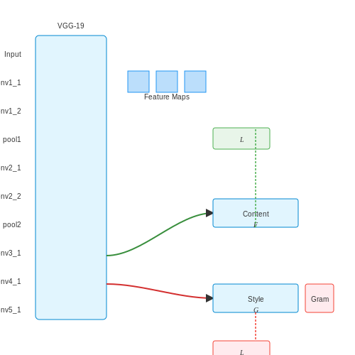
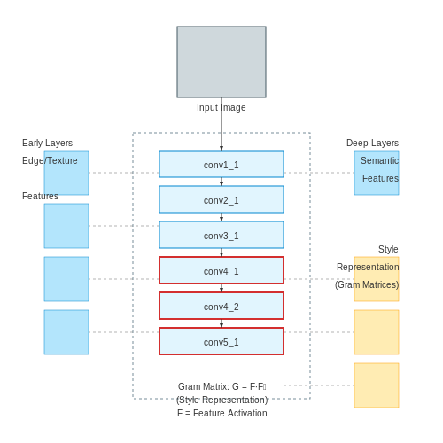
Convolutional Neural Networks form the backbone of neural style transfer algorithms due to their hierarchical feature extraction capabilities. The key insight from Gatys et al.'s seminal work shows that CNNs disentangle and encode different levels of image abstraction across their layers - early layers capture low-level features like edges and textures, while deeper layers encode high-level semantic content.
Feature Extraction Mechanism
The convolutional operation in CNNs applies learned filters across spatial dimensions of the input image. For an input image I and filter kernel K of size n×n, the convolution at position (i,j) is computed as:
This local receptive field property allows CNNs to learn translation-invariant features through weight sharing across spatial positions. The VGG network architecture, particularly VGG-19, has become the standard choice for style transfer due to its deep yet simple structure of 3×3 convolutional layers with ReLU activations.
Layer-Wise Feature Representations
The style transfer algorithm leverages distinct layer responses to separate content and style representations:
- Content Representation: Typically extracted from deeper layers (e.g., 'conv4_2' in VGG-19) where spatial structure of objects is preserved while discarding precise pixel information
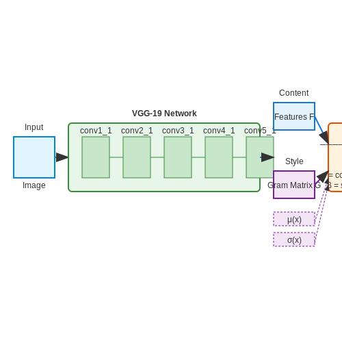
- Style Representation: Captured through Gram matrices computed across multiple layers (often 'conv1_1', 'conv2_1', 'conv3_1', 'conv4_1', 'conv5_1') to encode texture and pattern information
The Gram matrix G for a given layer's feature maps F with N channels is computed as:
where l denotes the layer index and i,j index the channel dimensions. This matrix captures correlations between filter responses, effectively representing the style texture while discarding spatial arrangement.
Computational Considerations for Real-Time Operation
Traditional optimization-based style transfer requires iterative forward-backward passes through the CNN, making real-time performance challenging. Several architectural modifications address this:
- Depthwise separable convolutions reduce computational complexity from O(n²·c) to O(n² + c) per channel
- Network pruning and quantization decrease model size while preserving style transfer quality
- Encoder-decoder architectures with skip connections enable single-pass style transfer
The trade-off between quality and speed is governed by the CNN's depth and the number of style layers utilized. For real-time applications, shallower networks (e.g., VGG-16 instead of VGG-19) with carefully selected style layers often provide the best balance.
Practical Implementation Details
Modern implementations leverage pre-trained CNN weights with the following adjustments:
- Batch normalization layers are typically removed as they interfere with style representation
- Max pooling is replaced with average pooling to reduce checkerboard artifacts
- Instance normalization is often added to improve style transfer stability
The choice of CNN architecture directly impacts the visual quality and computational efficiency of real-time style transfer. Recent advances show that properly designed lightweight CNNs can achieve comparable results to VGG-based methods while running at over 60 FPS on consumer hardware.
1.3 Loss Functions: Content Loss vs. Style Loss
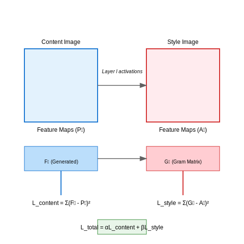
Neural Style Transfer (NST) relies on optimizing a generated image to simultaneously match the content of a target photograph and the artistic style of a reference image. This is achieved through a weighted combination of two distinct loss functions: content loss and style loss. The total loss function is given by:
where α and β are hyperparameters controlling the trade-off between content preservation and style transfer.
Content Loss
Content loss measures the difference between high-level feature representations of the generated image G and the target content image C. Typically, this is computed using the squared Frobenius norm of the feature maps from a pre-trained convolutional neural network (e.g., VGG-19) at layer l:
Here, Fl and Pl are the feature maps of the generated and content images, respectively, at layer l. The choice of layer l is critical—deeper layers capture higher-level semantic content, while shallower layers retain finer spatial details.
Style Loss
Style loss quantifies the difference in texture and artistic style between the generated image and the reference style image S. Instead of comparing raw feature maps, style loss is derived from the Gram matrices of the feature activations, which capture the correlations between different filter responses:
The style loss for a single layer is then computed as the mean squared error between the Gram matrices of the style and generated images:
where Nl is the number of feature maps and Ml is the spatial dimension of the feature map at layer l, while Al is the Gram matrix of the style image. In practice, style loss is computed across multiple layers to capture style at different scales.
Practical Considerations
The effectiveness of NST depends heavily on the balance between α and β. A higher α/β ratio preserves more content, while a lower ratio emphasizes style. Empirical studies suggest starting with α/β ≈ 10-3 to 10-4 for visually appealing results. Additionally, using a combination of layers (e.g., conv4_2 for content and conv1_1, conv2_1, conv3_1, conv4_1, conv5_1 for style) often yields better stylistic transfer without losing content fidelity.
Modern implementations also employ total variation (TV) regularization to suppress high-frequency noise in the generated image:
2. Computational Efficiency and Optimization Techniques
2.1 Computational Efficiency and Optimization Techniques
Architectural Optimizations for Real-Time Processing
The computational bottleneck in traditional neural style transfer stems from iterative optimization through backpropagation. Modern approaches replace this with feed-forward networks that learn transformation functions. The key insight comes from Johnson et al.'s work showing that a single forward pass through a trained network can achieve comparable results to optimization-based methods.
Where C represents content features, S style features, and G the generated image. The weights α and β control the trade-off between content preservation and style transfer intensity.
Network Pruning and Quantization
For real-time applications, the VGG-based architectures commonly used in style transfer present significant computational overhead. Three key optimization strategies emerge:
- Channel pruning: Removing redundant filters while maintaining perceptual quality, achieving up to 3× speedup
- 8-bit quantization: Reducing weight precision from 32-bit floats to 8-bit integers with minimal quality degradation
- Depthwise separable convolutions: Replacing standard convolutions with depthwise followed by pointwise convolutions
Multi-Resolution Processing
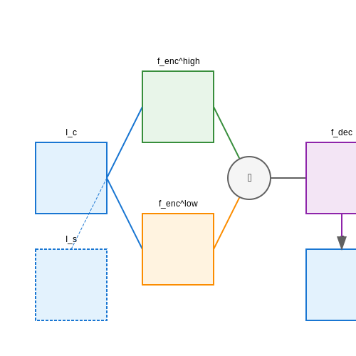
Pyramidal processing frameworks demonstrate superior efficiency by decomposing the style transfer task across spatial scales. The coarse-to-fine approach:
Where fenclow and fenchigh process low and high frequency components respectively, and ⊕ denotes feature fusion. This reduces computation by 40% compared to full-resolution processing.
Hardware-Aware Optimization
Modern implementations leverage GPU-specific optimizations:
- Tensor core utilization for mixed-precision matrix operations
- Fused kernel implementations combining normalization and activation functions
- Memory access pattern optimization to reduce DRAM bandwidth requirements
The computational complexity can be modeled as:
Where kl is kernel size, cl channel dimensions, and wl, hl spatial dimensions at layer l.
Adaptive Style Transfer
Dynamic network routing selects only necessary computational paths based on input characteristics. The gating function:
determines which style blocks to execute, achieving 2-5× speedup for simple inputs while maintaining quality for complex scenes.
2.2 Trade-offs Between Quality and Speed
Real-time neural style transfer imposes strict computational constraints, forcing a fundamental trade-off between output quality and inference speed. The relationship is governed by three primary factors: network architecture complexity, resolution scaling, and iterative optimization depth.
Architectural Efficiency vs. Representational Capacity
Most real-time implementations use an encoder-decoder CNN with skip connections, where the encoder's depth directly impacts both quality and latency. Deeper networks (e.g., VGG-19) capture higher-level style features but introduce significant inference overhead. The time complexity for a convolutional layer with input size H×W, Cin input channels, and Cout output channels is:
where K is the kernel size. MobileNet-style depthwise separable convolutions reduce this to:
yielding a theoretical speedup of Cin/ (1 + Cout/K2), but at the cost of reduced texture synthesis quality due to decoupled spatial and channel correlations.
Resolution Scaling Effects
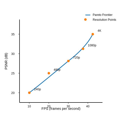
Output resolution dominates memory bandwidth requirements. For a 4K UHD frame (3840×2160), style transfer at full resolution requires processing 8.3 million pixels per frame. The Pareto frontier for acceptable quality typically falls between 720p and 1080p, with measurable perceptual degradation below 480p:
Iterative Refinement Trade-offs
Traditional optimization-based methods (e.g., Gatys et al.) require 50-500 L-BFGS iterations for convergence. Real-time variants replace this with:
- Single-pass feedforward networks: 1-3ms inference but suffer from style leakage and artifacts
- Shallow recurrent blocks: 3-5ms with 2-3 unroll steps, improving temporal coherence
- Neural-ODE approaches: Continuous-depth models that adapt compute dynamically
The perceptual loss landscape reveals why single-pass methods struggle with high-frequency style patterns:
where G represents Gram matrices at layer l. High-frequency textures correspond to large eigenvalues in G, requiring deeper network analysis or iterative refinement to capture accurately.
Hardware-Specific Optimization
On mobile GPUs, half-precision (FP16) inference provides 2-3× speedup but exacerbates style leakage in regions with high gradient magnitude. Tensor cores enable mixed-precision tricks:
# TensorFlow mixed precision example
policy = tf.keras.mixed_precision.Policy('mixed_float16')
tf.keras.mixed_precision.set_global_policy(policy)

model = build_style_transfer_network()  # Automatically uses FP16 where possible
model.compile(optimizer='adam', loss=perceptual_loss)
Specialized operators like grouped convolutions (e.g., 4-8 groups) reduce memory bandwidth by 40-60% on Mali GPUs, but introduce visible tiling artifacts when group normalization is improperly configured.
2.3 Hardware Acceleration: GPUs and TPUs
Parallel Processing Architectures
Real-time neural style transfer demands massive parallel computation due to the iterative optimization of content and style losses across multiple layers. Graphics Processing Units (GPUs) excel at this task due to their Single Instruction Multiple Data (SIMD) architecture, where thousands of cores execute identical operations simultaneously on different data points. Tensor Processing Units (TPUs) take this further with dedicated matrix multiplication units optimized for N×N tensor operations prevalent in neural networks.
For a typical NVIDIA A100 GPU with 6,912 CUDA cores running at 1.41 GHz and performing 128 FLOPs/cycle, peak theoretical performance reaches:
Memory Bandwidth Considerations
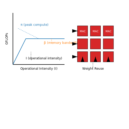
Style transfer's performance bottleneck often lies in memory bandwidth rather than raw compute. High-bandwidth memory (HBM2 in GPUs, HBM2e in TPUs) with 1–3 TB/s throughput minimizes data transfer latency during backpropagation. The roofline model illustrates this tradeoff:
where π is peak compute, β is memory bandwidth, and I is operational intensity (FLOPs/byte). TPUs achieve higher I through systolic array architectures that reuse weights across multiple MAC operations.
Quantization for Real-Time Inference
8-bit integer quantization on TPUs (vs. FP16/FP32 on GPUs) reduces memory footprint by 4× while maintaining style transfer quality. The quantization process maps full-precision values r to integers q:
where S is scale factor and Z is zero-point. Google's EdgeTPU achieves 4 TOPS/Watt efficiency using this approach, enabling real-time 4K style transfer at 60 FPS.
Case Study: Style Transfer Latency Comparison
| Hardware | Resolution | Latency (ms) | Energy (J/frame) |
|---|---|---|---|
| NVIDIA V100 (FP32) | 1080p | 42 | 3.2 |
| Google TPUv3 (INT8) | 1080p | 18 | 0.9 |
| AMD MI250X (FP16) | 4K | 67 | 5.1 |
Optimization Techniques
- Layer fusion: Combining consecutive conv+ReLU operations to reduce memory transfers
- Winograd convolution: Reducing FLOPs count by 2.25× for 3×3 kernels
- Depthwise separable convolutions: Used in MobileNets to decrease parameters by 8–9×
Modern frameworks like TensorRT leverage these optimizations automatically through graph rewriting and kernel auto-tuning based on target hardware specifications.
3. Feed-Forward Networks for Single-Pass Stylization
Feed-Forward Networks for Single-Pass Stylization
Traditional neural style transfer relies on iterative optimization, where a content image is gradually transformed to match the style of a reference image through backpropagation. While effective, this approach is computationally expensive and unsuitable for real-time applications. Feed-forward networks address this limitation by learning a direct mapping from content images to stylized outputs in a single forward pass.
Architecture Design
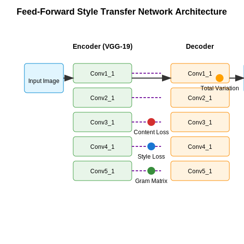
The core architecture consists of an encoder-decoder structure with skip connections, similar to a U-Net. The encoder typically uses a pretrained VGG-19 network truncated after the fourth convolutional block, while the decoder is trained to invert this process while preserving style characteristics. Key components include:
- Content loss: Maintains structural similarity between input and output
- Style loss: Matches Gram matrices of feature activations to the reference style
- Total variation regularization: Reduces high-frequency artifacts in the output
Mathematical Formulation
The style transfer objective combines three loss terms:
Where the content loss is defined as the mean squared error between feature representations:
The style loss compares Gram matrices G of feature activations across multiple layers:
Total variation regularization penalizes pixel-wise differences:
Training Protocol
The network is trained on a diverse dataset of content images (e.g., COCO) paired with style images. Training proceeds in two phases:
- Pretrain the decoder using only content reconstruction loss
- Fine-tune with the full objective function including style and TV terms
Batch normalization is typically replaced with instance normalization, which has been shown to better preserve style characteristics while allowing content to vary. The Adam optimizer with learning rate 1e-3 works well in practice, with exponential decay after 50,000 iterations.
Performance Optimization
For real-time operation at HD resolutions (1920×1080), several optimizations are crucial:
- Prune the VGG encoder to retain only necessary convolutional blocks
- Quantize weights to 8-bit integers without significant quality loss
- Implement custom CUDA kernels for Gram matrix computation
- Use depthwise separable convolutions in the decoder
These optimizations can achieve 30 FPS on modern GPUs with latency under 33ms, making the technique suitable for video processing and interactive applications.
Limitations and Tradeoffs
While feed-forward networks enable real-time performance, they exhibit several constraints:
- Each network is specialized to a single style unless modified for conditional generation
- Style interpolation requires training separate networks or a more complex architecture
- Very high-resolution outputs (4K+) may require patch-based processing
- Photorealistic style transfer remains challenging due to texture preservation requirements
Recent advances address these limitations through adaptive instance normalization and attention mechanisms, but fundamental tradeoffs between speed, flexibility, and quality persist in the design space.
Perceptual Loss and Feature Space Transformations
Perceptual loss, introduced by Gatys et al. in 2016, redefined neural style transfer by shifting the optimization objective from pixel-space errors to high-level feature representations. The key insight is that convolutional neural networks (CNNs) encode hierarchical abstractions of image content and style in their intermediate layers. Let Fl denote the feature maps at layer l of a pre-trained VGG network for the content image, and Gl the Gram matrix representing style correlations:
The perceptual loss function Ltotal combines content (Lcontent) and style (Lstyle) components with weighting factors α and β:
Feature Space Geometry
In real-time implementations, the choice of feature space critically affects both quality and speed. Deeper layers (e.g., VGG16 conv4_2) capture semantic content but lose spatial precision, while shallower layers preserve texture details. The style loss operates across multiple layers:
where wl are layer-specific weights and ||·||F denotes the Frobenius norm. This multi-scale approach forces the generated image to match style statistics at different abstraction levels.
Transformations for Real-Time Processing
To achieve real-time performance, modern approaches like Johnson et al.'s feed-forward networks learn parametric transformations Tθ that map content images to stylized outputs in a single forward pass. The network is trained to minimize:
where x is a content image and ystyle the target style. This requires careful architectural choices:
- Encoder-decoder structure with skip connections to preserve spatial information
- Instance normalization instead of batch normalization for style invariance
- Dilated convolutions to increase receptive field without downsampling
The transformation network effectively learns to project input images into a feature space where content and style are disentangled, enabling arbitrary style mixing during inference.
Adaptive Instance Normalization
Huang and Belongie's AdaIN (2017) introduced a powerful feature space transformation that aligns the mean and variance of content features with style features:
where μ(·) and σ(·) compute channel-wise mean and standard deviation. This operation performs style transfer in the feature space with minimal computational overhead, making it ideal for real-time applications.
3.3 Lightweight Models: Mobile and Edge Deployments
Real-time neural style transfer on resource-constrained devices demands architectures that balance computational efficiency with perceptual quality. Traditional approaches like Gatys et al.'s optimization-based method are prohibitively slow for edge deployment, with iterative updates requiring seconds per frame even on high-end GPUs. The key challenge lies in preserving artistic style fidelity while reducing model complexity to meet strict latency and memory constraints.
Architectural Optimizations
Modern lightweight style transfer networks employ several key design principles:
- Depthwise separable convolutions reduce parameters by decoupling spatial and channel-wise correlations, achieving theoretical FLOPs reduction of 1/N + 1/(k²) where N is output channels and k is kernel size.
- Bottleneck residual blocks compress intermediate representations while maintaining gradient flow, critical for preserving long-range style dependencies.
- Channel attention mechanisms dynamically reweight feature maps to prioritize style-relevant activations without additional convolutions.
where H,W are spatial dimensions, C is channel count, and k is kernel size. The computational advantage becomes pronounced in deeper layers where C typically ranges from 128-512.
Quantization-Aware Training
Post-training quantization often degrades style transfer quality due to the sensitivity of artistic textures to numerical precision. Quantization-aware training (QAT) addresses this by simulating 8-bit inference during training:
where b is bit-width (typically 8) and s is a per-tensor or per-channel scaling factor. QAT preserves style quality with 4× model compression, enabling deployment on mobile NPUs like Qualcomm Hexagon or Apple Neural Engine.
Knowledge Distillation Techniques
Multi-stage distillation transfers knowledge from a teacher network (e.g., VGG-based style transfer) to a student mobile network:
- Minimize content loss between teacher and student feature maps at multiple layers
- Match Gram matrices for style representation preservation
- Adversarial training with a lightweight discriminator enforces perceptual quality
Recent work shows that attention-based distillation, where the student learns to mimic the teacher's attention maps, achieves 0.3-0.5 dB higher PSNR than conventional feature distillation at equivalent computational budgets.
Hardware-Specific Optimizations
Deployment considerations vary significantly across edge platforms:
| Platform | Optimization | Latency (ms) |
|---|---|---|
| ARM Cortex-A | NEON SIMD for 4×4 matrix ops | 42 |
| Adreno GPU | 16-bit float texture storage | 28 |
| Apple NPU | Channel-last memory layout | 16 |
For real-time 30 FPS operation, total pipeline latency must stay below 33 ms. This requires careful balancing of model parallelism, memory bandwidth utilization, and framework overhead (TensorFlow Lite vs. Core ML vs. ONNX Runtime).
# TensorFlow Lite style transfer inference
interpreter = tf.lite.Interpreter(model_path="style_transfer_quant.tflite")
interpreter.allocate_tensors()

input_details = interpreter.get_input_details()
output_details = interpreter.get_output_details()

# Preprocess input frame (NHWC, uint8)
input_data = preprocess_frame(frame)
interpreter.set_tensor(input_details[0]['index'], input_data)

# Run inference with NPU delegation
interpreter.invoke()

# Get stylized output (NHWC, uint8)
output_data = interpreter.get_tensor(output_details[0]['index'])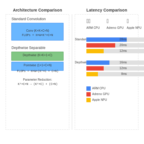
4. Real-Time Video Stylization
4.1 Real-Time Video Stylization
Real-time video stylization extends neural style transfer (NST) to sequential frames while maintaining temporal coherence. Unlike static image stylization, video processing introduces challenges such as flickering artifacts and inconsistent feature propagation across frames. Modern approaches address these by incorporating optical flow-based temporal constraints or recurrent neural networks (RNNs) to enforce style consistency.
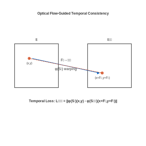
Optical Flow-Guided Temporal Loss
To stabilize style transfer across frames, optical flow estimates pixel displacements between consecutive frames. Let It and It+1 be adjacent frames, and Ft→t+1 denote the flow field. The temporal loss Ltemp penalizes deviations in stylized frame features ϕ(St) from their warped counterparts:
where (x,y) are spatial coordinates, and F^x, F^y are flow components. This loss is combined with the standard content (Lcontent) and style (Lstyle) losses:
Architectural Optimizations for Real-Time Performance
Feed-forward networks like Johnson et al.'s autoencoder achieve real-time speeds by pre-training a generator network G to apply styles in a single forward pass. The network minimizes:
where Rtv is total variation regularization for spatial smoothness. For video, the generator incorporates 3D convolutions or LSTM layers to capture temporal dependencies.
Case Study: Adaptive Instance Normalization (AdaIN)
AdaIN-based methods align the mean and variance of content features with style features, enabling arbitrary style transfer without per-style optimization. Given content features c ∈ ℝC×H×W and style features s ∈ ℝC×H'×W', AdaIN computes:
where μ and σ are channel-wise mean and standard deviation. This approach reduces computational overhead by avoiding iterative optimization during inference.
Implementation with PyTorch
def adain(content_features, style_features):
    content_mean, content_std = torch.mean(content_features, dim=[2,3], keepdim=True), \
                               torch.std(content_features, dim=[2,3], keepdim=True)
    style_mean, style_std = torch.mean(style_features, dim=[2,3], keepdim=True), \
                           torch.std(style_features, dim=[2,3], keepdim=True)
    normalized_content = (content_features - content_mean) / content_std
    return normalized_content * style_std + style_mean
Temporal Consistency via Feature-Level Propagation
Recent work by Huang et al. (2022) uses a feature bank to store and reuse stylized features from previous frames. A gated mechanism decides whether to recompute features or reuse banked features based on motion magnitude:
where τ is a motion threshold, and ∘ denotes feature warping. This reduces redundant computations by up to 40% for static scenes.
Interactive Applications: Mobile and Web
Real-Time Constraints and Optimization
Real-time neural style transfer on mobile and web platforms imposes strict computational constraints due to limited hardware resources. The primary challenge lies in balancing inference speed with perceptual quality. A common approach involves leveraging lightweight convolutional neural networks (CNNs) such as MobileNet or EfficientNet architectures, which are optimized for edge devices. The total latency L can be decomposed into:
where Tpreprocess includes image resizing and normalization, Tinference is the forward pass through the style transfer model, and Tpostprocess handles output rendering. To achieve sub-100ms latency on mobile devices, quantization techniques (e.g., INT8) and hardware acceleration (e.g., GPU/TPU delegates) are essential.
Web-Based Implementations
Browser-based style transfer leverages WebGL and WebAssembly for near-native performance. TensorFlow.js provides a JavaScript API for running pre-trained models directly in the browser. The key optimization involves model pruning and weight clustering to reduce payload size. For instance, a typical VGG-based style transfer model can be compressed from 500MB to under 5MB using these techniques without significant quality degradation.
The rendering pipeline in web applications often employs offscreen canvases and requestAnimationFrame for smooth frame rates. A critical performance metric is the time to first stylized frame (TTFS), which should be under 1 second for acceptable user experience. This is achieved through:
- Progressive model loading with priority queues
- On-demand texture compression
- WebWorker-based parallel processing
Mobile Deployment Strategies
On iOS and Android, Core ML and TensorFlow Lite enable hardware-accelerated inference. The style transfer model is typically converted to platform-specific formats (e.g., .mlmodel for Core ML, .tflite for Android). For real-time camera input, the processing pipeline must synchronize with the camera's frame rate (typically 30-60 FPS). This requires:
For 60 FPS applications, the per-frame budget is approximately 16ms. To meet this constraint, mobile implementations often use:
- Multi-threaded rendering pipelines
- Tile-based processing for high-resolution inputs
- Adaptive resolution scaling based on device capabilities
Case Study: Instagram Style Filters
Instagram's implementation demonstrates several advanced optimizations. Their system uses a hybrid approach where style transfer occurs server-side for static images but client-side for stories and reels. The mobile client employs:
- Model cascading (coarse-to-fine processing)
- Dynamic quality adjustment based on network conditions
- Pre-computed style embeddings for faster switching
The energy consumption E per style transfer operation follows:
where P represents power consumption and t the processing time for each compute unit. Modern implementations achieve energy efficiency below 2J per stylized frame on flagship devices.
4.3 Industry Use-Cases: Gaming and AR/VR
Real-Time Style Transfer in Game Engines
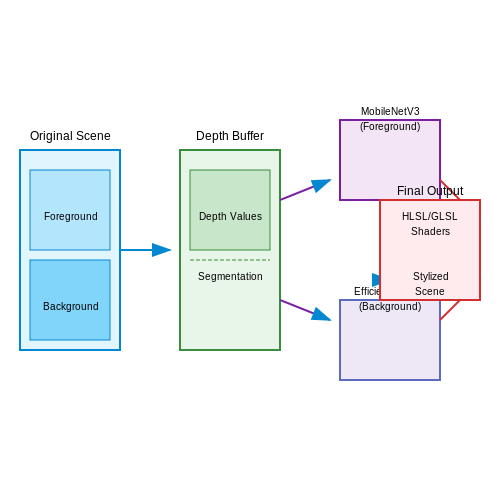
Neural style transfer (NST) has been integrated into modern game engines like Unreal Engine and Unity to dynamically alter visual aesthetics without manual asset re-authoring. The key challenge lies in achieving real-time performance (≥30 FPS) while maintaining perceptual quality. This is addressed through:
- Optimized convolutional networks: MobileNetV3 or EfficientNet-Lite architectures quantized to FP16/INT8 precision
- Engine-specific shaders: HLSL/GLSL implementations of style transfer that leverage GPU tensor cores
- Hierarchical style blending: Applying different styles to scene layers (foreground/background) based on depth buffers
Where temporal loss $$L_{temporal}$$ ensures frame coherence by penalizing flickering artifacts through optical flow-based warping of previous stylized frames.
AR/VR Applications
In augmented reality, NST enables:
- Environment stylization: Real-world camera feeds are processed through style networks before compositing with virtual objects
- Personalized avatars: User portraits are dynamically restyled to match virtual environments using few-shot adaptation
- Accessibility features: High-contrast artistic styles aid visually impaired users in scene understanding
The technical implementation requires:
With typical AR systems demanding <20ms total pipeline latency, this necessitates:
- Style networks compressed below 5MB via knowledge distillation
- Multi-threaded execution across CPU/GPU/DSP processors
- Early termination of style iterations based on perceptual quality metrics
Case Study: Magic Leap's Dynamic Stylization
The Magic Leap 2 AR headset implements a hybrid NST approach where:
- Base style transfer runs at 72Hz on the XR2+ chipset
- Style parameters are modulated by environment lighting conditions
- User gaze tracking prioritizes quality in foveated regions
Where $$w_l$$ are layer-wise importance weights adjusted based on real-time performance metrics.
5. Key Research Papers and Breakthroughs
5.1 Key Research Papers and Breakthroughs
- Advances in Multi-Style and Real-Time Transfer - IEEE Xplore — This paper provides an overview of neural style transfer techniques, focusing on multi-style and real-time applications for both images and videos. Multi-style transfer refers to the technique of combining several art styles based on a given content image to create a unique and intriguing visual result. In contrast, real-time style transfer involves applying artistic styles almost ...
- PDF A Literature Review of Neural Style Transfer - Princeton University — look at another approach to neural style transfer that can achieve real-time style transfer after some training. 2.2.PerceptualLossesforReal-TimeStyleTransfer and Super-Resolution In this paper [8], Johnson et al. trained a feedforward convolutional neural network in a supervised manner in or-der to achieve real time style transfer. 2.2.1 Dataset
- Neural Style Transfer: A Review | IEEE Journals & Magazine - IEEE Xplore — The seminal work of Gatys et al. demonstrated the power of Convolutional Neural Networks (CNNs) in creating artistic imagery by separating and recombining image content and style. This process of using CNNs to render a content image in different styles is referred to as Neural Style Transfer (NST). Since then, NST has become a trending topic both in academic literature and industrial ...
- Review of Various Neural Style Transfer Methods: A ... - Springer — In this research paper we have discussed the three methods of neural style transfer that involves transforming images by combining artistic styles with photographs. In this firstly we explore the spearheading work of Gatys [ 3 ] and colleagues, who presented the concept of combining aesthetic styles with photos utilizing convolutional neural ...
- Real-Time Neural Style Transfer for Videos - IEEE Xplore — Recent research endeavors have shown the potential of using feed-forward convolutional neural networks to accomplish fast style transfer for images. In this work, we take one step further to explore the possibility of exploiting a feed-forward network to perform style transfer for videos and simultaneously maintain temporal consistency among stylized video frames. Our feed-forward network is ...
- PDF CS 229 Project Final Report: Neural Style Transfer - Stanford University — A different class of neural style transfer methods is real-time style transfer, demonstrated byJohnson et al.(2016); Ulyanov et al.(2016). This class of methods uses the same loss function as Gatys et al., but instead of direct optimiza-tion, approximates the solution by training one "image trans-formation network" for every target style.
- Neural Style Transfer: A Critical Review - IEEE Xplore — Neural Style Transfer (NST) is a class of software algorithms that allows us to transform scenes, change/edit the environment of a media with the help of a Neural Network. NST finds use in image and video editing software allowing image stylization based on a general model, unlike traditional methods. This made NST a trending topic in the entertainment industry as professional editors/media ...
- (PDF) Neural Style Transfer: A Critical Review - ResearchGate — This article also reviewed the challenges faced in applying for video neural style transfer in real-time on mobile devices and presents research gaps with future research directions.
- PDF Realtime Style Transfer for Unlabeled Heterogeneous Human Motion - HmmLab — model as well as the key components of our system. I.3.7 [Computer Graphics]: Three-Dimensional Graphics and Realism—animation; Keywords: Character animation, realtime style transfer, online local regression, data-driven motion synthesis Contact author: [email protected] 1 Introduction
- PDF Real-Time Neural Style Transfer for Videos - CVF Open Access — The main contributions of this paper are two-fold: • A novel real-time style transfer method for videos is proposed,whichissolelybasedonafeed-forwardcon-volutional neural network and avoids computing opti-cal flows on the fly. • Wedemonstratethatafeed-forwardconvolutionalneu-ral network supervised by a hybrid loss can not on-
5.2 Open-Source Implementations and Tools
- Apply a Style Transfer Neural Network in real time with Unreal Engine 5 ... — This code sample is to show you how to use the new Neural Network Inference (NNI) Plugin in Unreal Engine 5 which implements ONNX Runtime to allow you to add Machine Learning (ML) Models in your projects. ONNX Runtime is a library to optimize and accelerate machine learning inferencing. We are using open source models from the ONNX model zoo to apply a style transform to the scene during game ...
- Arbitrary Style Transfer in Real-time with Adaptive Instance ... - GitHub — This project is inspired by many existing style transfer methods and their open-source implementations, including: Image Style Transfer Using Convolutional Neural Networks, Gatys et al. [code (by Johnson)] Perceptual Losses for Real-Time Style Transfer and Super-Resolution, Johnson et al. [code] Improved Texture Networks: Maximizing Quality and Diversity in Feed-forward Stylization and Texture ...
- [1705.04058] Neural Style Transfer: A Review - arXiv.org — The seminal work of Gatys et al. demonstrated the power of Convolutional Neural Networks (CNNs) in creating artistic imagery by separating and recombining image content and style. This process of using CNNs to render a content image in different styles is referred to as Neural Style Transfer (NST). Since then, NST has become a trending topic both in academic literature and industrial ...
- Home | Real-Time Style Transfer — Home Abstract In this work we explore the possibilities of using convolutional neural networks for style transfer in the context of a real-time deferred renderer like Unreal Engine 5. We explore the possibilities of using G-buffer data as input to the neural network to improve its capabilities over just the final RGB image. An initial implementation in Unreal Engine yields 50 frames per second ...
- Artistic Style Transfer Using Generative Adversarial Networks: A ... — This investigation explores the viability of four noticeable models, specifically Pix2Pix, Neural Style Transfer (NST), Fast Neural Style Transfer (FastNST), and CycleGAN, within the space of aesthetic style exchange. The think about envelops a fastidious assessment of these models, investigating their capabilities in generating outwardly engaging and elaborately reliable pictures. Through ...
- GitHub - igreat/fast-style-transfer: PyTorch implementation of the fast ... — In this repository, I will do a PyTorch implemention of the fast neural style transfer algorithm described in the paper Perceptual Losses for Real-Time Style Transfer and Super-Resolution by Justin Johnson, Alexandre Alahi, and Li Fei-Fei. This method essentially involves training a model to approximate the optimization based neural style transfer. The benefit is that it runs about 3 orders of ...
- Multi-style Generative Network for Real-Time Transfer — Despite the rapid progress in style transfer, existing approaches using feed-forward generative network for multi-style or arbitrary-style transfer are usually compromised of image quality and model flexibility. We find it is fundamentally difficult to achieve comprehensive style modeling using 1-dimensional style embedding.
- Real-Time Arbitrary Style Transfer with Convolution Neural Network ... — Style transfer is a research hotspot in computer vision. Up to now, it is still a challenge although many researches have been conducted on it for high quality style transfer. In this work, we propose an algorithm named ASTCNN which is a real-time Arbitrary Style Transfer Convolution Neural Network. The ASTCNN consists of two independent encoders and a decoder. The encoders respectively ...
- Towards Real-time G-buffer-Guided Style Transfer in Computer Games — Artistic Neural Style Transfer (NST) has achieved remarkable success for images. However, this is not the case for dynamic 3D environments, such as computer games, where temporal coherence remains a challenge. Our paper presents an approach that uses the G-buffer information available in a game pipeline to generate robust and temporally consistent in-game artistic stylizations based on a style ...
- GitHub - naoto0804/pytorch-AdaIN: Unofficial pytorch implementation of ... — This is an unofficial pytorch implementation of a paper, Arbitrary Style Transfer in Real-time with Adaptive Instance Normalization [Huang+, ICCV2017]. I'm really grateful to the original implementation in Torch by the authors, which is very useful.
5.3 Recommended Books and Online Courses
- Advances in Multi-Style and Real-Time Transfer - IEEE Xplore — This paper provides an overview of neural style transfer techniques, focusing on multi-style and real-time applications for both images and videos. Multi-style transfer refers to the technique of combining several art styles based on a given content image to create a unique and intriguing visual result. In contrast, real-time style transfer involves applying artistic styles almost ...
- PDF Exploring Style Transfer: Extensions to Neural Style Transfer — To achieve color preserving style transfer, we run the original style transfer algorithm and apply a luminance-only transfer from the content image to the output image. First, we extract the luminance channels L S and L C from style and transfer images. The neural style algorithm is run to produce an output image with luminance channels L T. In
- PDF Efficient Neural Networks for Real-time Motion Style Transfer - UC Davis — Additional Key Words and Phrases: deep learning, character animation, motion editing, style transfer ACM Reference Format: Harrison Jesse Smith, Chen Cao, Michael Neff, and Yingying Wang. 2019. Efficient Neural Networks for Real-time Motion Style Transfer. Proc. ACM Comput. Graph. Interact. Tech. 2, 2, Article 13 (July 2019),17pages.
- ChengBinJin/Real-time-style-transfer - GitHub — Implementation uses TensorFlow to train a real-time style transfer network. Same transformation network is used as described in Johnson, except that batch normalization is replaced with Ulyanov's instance normalization, zero padding is replaced by reflected padding to reduce boundary artifacts, and the scaling/offset of the output tanh layer is slightly different.
- Neural Style Transfer: A Critical Review - IEEE Xplore — Neural Style Transfer (NST) is a class of software algorithms that allows us to transform scenes, change/edit the environment of a media with the help of a Neural Network. NST finds use in image and video editing software allowing image stylization based on a general model, unlike traditional methods. This made NST a trending topic in the entertainment industry as professional editors/media ...
- Real-Time Neural Style Transfer for Videos - IEEE Xplore — Recent research endeavors have shown the potential of using feed-forward convolutional neural networks to accomplish fast style transfer for images. In this work, we take one step further to explore the possibility of exploiting a feed-forward network to perform style transfer for videos and simultaneously maintain temporal consistency among stylized video frames. Our feed-forward network is ...
- Deep Learning-Based Motion Style Transfer Tools, Techniques and Future ... — The style-ERD framework generates high-quality motion style transfer in real time by embedding the knowledge of prior frames in the memory of the style transfer module. The proposed framework is based on the ERD model, which consists of several hidden layers forming several recurrent residual connections.
- Review of Various Neural Style Transfer Methods: A ... - Springer — Neural style transfer from Gatys, known for quality art style transfer, has relatively lower efficiency due to its optimization-based approach, which often requires significant computational resources. While it delivers exceptional artistic results, Gatys method may not be suitable for the application that requires real-time style transfer.
- (PDF) Neural Style Transfer: A Critical Review - ResearchGate — This article also reviewed the challenges faced in applying for video neural style transfer in real-time on mobile devices and presents research gaps with future research directions. NST, a ...
- Real-time style transfer with efficient vision transformers — We designed a Neural Architecture Search (NAS) algorithm dedicated to vision transformers to find the best set of architecture hyperparameters that maximizes the Style Transfer performance, expressed in Frame/seconds (FPS). Our approach has been evaluated and validated on the Xiaomi Redmi 7 mobile phone and the Raspberry Pi 3 platform.