Evaluating Robustness in Vision Models
1. Defining Robustness: Key Concepts and Metrics
1.1 Defining Robustness: Key Concepts and Metrics
Robustness in vision models refers to their ability to maintain performance under distributional shifts, adversarial perturbations, or noisy inputs. Unlike accuracy, which measures performance on i.i.d. test data, robustness evaluates generalization under non-i.i.d. conditions. Key dimensions include:
1. Adversarial Robustness
Adversarial robustness quantifies a model’s resilience to worst-case perturbations. Given an input image $$x$$ and classifier $$f$$, the adversarial example $$x'$$ is crafted to maximize the loss $$L(f(x'), y)$$ while constraining $$||x' - x||_p \leq \epsilon$$. Common norms include:
Metrics like Adversarial Accuracy measure the fraction of test samples correctly classified after perturbation.
2. Corruption Robustness
Models are evaluated on synthetically corrupted data (e.g., Gaussian noise, motion blur). The Corruption Error (CE) is computed as:
where $$\delta$$ is a corruption operator. Benchmarks like ImageNet-C standardize this evaluation.
3. Domain Shift Robustness
Measures performance under natural distribution shifts (e.g., lighting changes, geographic variations). Key metrics include:
- Relative Performance Drop (RPD): $$\frac{\text{Accuracy}_{\text{source}} - \text{Accuracy}_{\text{target}}}{\text{Accuracy}_{\text{source}}}$$
- Area Under the Risk-Change Curve (AURC): Integrates performance across increasing shift severity.
4. Calibration and Uncertainty
Robust models should output calibrated confidence scores. Expected Calibration Error (ECE) bins predictions by confidence and compares to empirical accuracy:
where $$B_m$$ is the m-th bin and $$n$$ is the sample count.
5. Gradient-Based Metrics
Sensitivity to input perturbations can be analyzed via gradient norms. The Jacobian Norm $$||J_f(x)||_F$$ (Frobenius norm of the model’s Jacobian) indicates local Lipschitzness—lower values suggest smoother decision boundaries.

1.2 Common Failure Modes in Vision Models
Adversarial Attacks
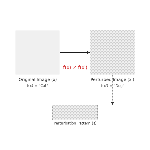
Vision models are particularly vulnerable to adversarial perturbations—small, often imperceptible noise patterns added to input images that cause misclassification. Formally, given an input image x and a target model f, an adversarial example x' satisfies:
where ε is a small perturbation budget under Lp norm constraints. Fast Gradient Sign Method (FGSM) and Projected Gradient Descent (PGD) are widely studied attack methods that exploit gradient information to craft perturbations. For instance, FGSM computes:
where J is the loss function and y is the true label. These attacks reveal that vision models often rely on non-robust features that humans disregard.
Distributional Shift
Models trained on i.i.d. data frequently fail under distribution shifts, such as:
- Covariate shift: Changes in input distribution P(x) while P(y|x) remains constant (e.g., daylight vs. night-time images).
- Label shift: Shifts in P(y) while P(x|y) stays fixed (e.g., rare classes becoming prevalent).
- Concept drift: Changes in P(y|x) over time (e.g., redefinition of diagnostic criteria in medical imaging).
The performance drop can be quantified using the Kullback-Leibler divergence between training and test distributions:
Texture Bias
Convolutional Neural Networks (CNNs) exhibit a strong bias toward texture over shape, as demonstrated by style-transfer experiments. When tested on images with conflicting shape and texture cues (e.g., elephant texture on a cat shape), models often classify based on texture alone. This stems from the inductive bias of local receptive fields in early convolutional layers, which prioritize high-frequency patterns.
Occlusion Sensitivity
Vision models degrade nonlinearly under partial occlusions. For a given occlusion mask M applied to image region Ω, the output logits z change as:
where ⊙ denotes element-wise multiplication. Critical failure occurs when Ω contains class-discriminative regions identified via saliency maps or Grad-CAM visualizations.
Contextual Overfitting
Models often exploit spurious correlations with contextual features (e.g., classifying cows based on grassy backgrounds). This becomes apparent when testing on out-of-context samples (e.g., cows on beaches) or via adversarial background perturbations. The phenomenon is quantified by comparing performance on original images versus context-ablated versions.
Quantization and Hardware Failures
Deployed models face additional failure modes from hardware constraints:
- Quantization artifacts: Reduced bit-depth (e.g., FP32 → INT8) introduces rounding errors that accumulate nonlinearly:
- Thermal noise: Analog components in vision sensors introduce Poisson-distributed noise that corrupts input signals.
The Role of Data Distribution in Model Robustness
Model robustness in vision systems is fundamentally tied to the statistical properties of the training data distribution. A model's ability to generalize to unseen inputs—particularly under distribution shifts—depends on how well the training set captures the underlying data manifold. The joint distribution P(X,Y), where X represents input images and Y their labels, must sufficiently cover the variations expected during deployment.
Data-Centric Factors Influencing Robustness
Three key properties of the data distribution determine robustness:
- Support Coverage: The extent to which the training data spans the test distribution. Incomplete coverage leads to brittle models that fail on out-of-distribution (OOD) samples.
- Label Consistency: The reliability of annotations across similar inputs. Noisy or inconsistent labels degrade decision boundaries.
- Feature Diversity: The variety of nuisance variables (lighting, occlusion, etc.) present during training. Limited diversity causes oversensitivity to these factors.
Quantifying Distribution Gaps
The discrepancy between training (Ptrain) and test (Ptest) distributions can be measured using divergence metrics. The Kullback-Leibler (KL) divergence provides a theoretically-grounded measure:
For continuous vision data, we often use the Wasserstein distance, which accounts for the geometric structure of image space:
where Γ represents all joint distributions with marginals Ptrain and Ptest, and d(x,y) is a distance metric (typically L2 for images).
Practical Implications for Dataset Construction
Modern robustness benchmarks like ImageNet-C and ObjectNet explicitly test distribution shift scenarios through:
- Controlled Corruptions: Systematic application of noise, blur, and digital artifacts
- Natural Variations: Changes in viewpoint, background, and illumination
- Adversarial Examples: Worst-case perturbations optimized to fool models
Training strategies must account for these factors through techniques such as domain randomization, where synthetic data spans a wider distribution than the expected test set. The effectiveness of this approach follows from the probably approximately correct (PAC) learning framework—expanding the training distribution's support reduces the generalization gap.
Case Study: Autonomous Vehicle Perception
In self-driving systems, the data distribution must cover rare but critical scenarios (e.g., pedestrians at night, adverse weather). The long-tail nature of real-world data requires either:
- Exponentially larger datasets to capture rare events
- Strategic oversampling of edge cases during training
- Generative augmentation to expand distribution support
Recent work has shown that models trained on synthetic data from physics-based simulators (e.g., CARLA) can achieve comparable robustness to real-world training when the simulator's parameter space sufficiently covers the test distribution's variability.

2. Types of Adversarial Attacks on Vision Models
2.1 Types of Adversarial Attacks on Vision Models
White-Box Attacks
White-box attacks assume complete knowledge of the target model, including its architecture, parameters, and gradients. The attacker leverages this information to craft perturbations that maximize the model's prediction error. One of the most widely studied white-box attacks is the Fast Gradient Sign Method (FGSM), which generates adversarial examples by linearizing the loss function J(θ, x, y) with respect to the input x:
Here, ϵ controls the perturbation magnitude. More sophisticated variants like Projected Gradient Descent (PGD) iteratively refine the perturbation under an Lp-norm constraint:
where Π denotes projection onto the feasible set 𝒮, and α is the step size. These attacks are particularly effective against convolutional neural networks (CNNs) and vision transformers.
Black-Box Attacks
Black-box attacks operate without access to the model's internal parameters. They rely on query-based strategies or transferability from surrogate models. Score-based attacks estimate gradients via finite differences:
where u is a random unit vector and δ is a small step size. Decision-based attacks, such as the Boundary Attack, modify inputs until they cross the decision boundary:
These attacks are computationally expensive but pose significant threats to real-world systems like autonomous vehicles and facial recognition.
Universal Adversarial Perturbations
Unlike input-specific perturbations, universal adversarial perturbations are designed to fool a model on most inputs from a data distribution. They solve the optimization problem:
where δ is the desired success rate. These perturbations exploit geometric correlations in decision boundaries across different inputs.
Physical-World Attacks
Physical attacks modify real-world objects to deceive vision systems under varying viewpoints and lighting conditions. Techniques include:
- Adversarial patches: Optimized textures placed in the scene
- Camouflage: Patterns that blend with backgrounds
- 3D adversarial objects: Printed objects that fool multiple viewpoints
These attacks raise critical security concerns for applications like traffic sign recognition and surveillance systems.
Certified Defenses and Robustness Metrics
Evaluating attack effectiveness requires rigorous metrics:
- Attack Success Rate (ASR): Fraction of inputs successfully misclassified
- Perturbation Magnitude: L2 or L∞ norms of adversarial noise
- Transferability: Cross-model attack success rates
Certified defenses provide mathematical guarantees against perturbations within a specified radius r:

2.2 Evaluating Model Vulnerability to Adversarial Examples
Adversarial examples are carefully perturbed inputs designed to deceive machine learning models while remaining imperceptible to human observers. Evaluating a vision model's robustness against such attacks involves quantifying its susceptibility under controlled adversarial conditions. The process typically consists of three key steps: attack generation, perturbation measurement, and robustness assessment.
Attack Generation Methods
White-box attacks assume full knowledge of the model architecture and parameters. The Fast Gradient Sign Method (FGSM) remains a fundamental approach, generating adversarial examples through a single step in the direction of the loss gradient:
where x is the original input, y the true label, J the loss function, and ϵ controls perturbation magnitude. More sophisticated iterative methods like Projected Gradient Descent (PGD) apply FGSM multiple times with smaller steps:
Black-box attacks, by contrast, operate without model internals. Transfer-based attacks leverage adversarial examples crafted on surrogate models, while score-based methods estimate gradients through query outputs. Decision-based attacks like the Boundary Attack perturb inputs until crossing decision boundaries.
Perturbation Metrics
The Lp norm family quantifies perturbation strength:
- L∞: Maximum pixel-wise difference (max|xi - xi'|)
- L2: Euclidean distance between original and adversarial examples
- L0: Count of modified pixels
Structural similarity metrics like SSIM assess perceptual quality degradation, while domain-specific measures (e.g., PSNR for images) provide application-relevant evaluations.
Robustness Assessment
Adversarial accuracy measures the model's performance under attack:
where f is the model and N the test set size. The robustness curve plots accuracy against increasing perturbation budgets, revealing failure thresholds. Certified robustness methods provide theoretical guarantees by calculating the largest perturbation radius r within which no adversarial example exists:
Empirical evaluations should test against diverse attack types and strengths, as robustness often varies significantly across threat models. The CleverHans library provides standardized benchmarks, while frameworks like RobustBench maintain leaderboards for comparing model performances.

2.3 Defensive Strategies: Adversarial Training and Robust Optimization
Adversarial Training
Adversarial training is a defense mechanism where a model is explicitly trained on adversarial examples to improve its robustness. The objective is to minimize the worst-case loss over a perturbation set, formalized as:
Here, θ represents the model parameters, Δ defines the allowable perturbation space (e.g., ℓ∞-bounded), and ℒ is the loss function. The inner maximization generates adversarial examples, while the outer minimization updates the model to resist them. Practical implementations often use Projected Gradient Descent (PGD) for the inner maximization:
where ΠΔ projects perturbations back into the feasible set Δ. This process is computationally expensive but empirically effective, as demonstrated by Madry et al. (2018) on CIFAR-10 and ImageNet.
Robust Optimization Variants
Standard adversarial training can overfit to specific attack types. Robust optimization techniques address this by:
- TRADES (Zhang et al., 2019): Decouples natural and adversarial loss terms:
$$ \min_\theta \mathbb{E}_{(x,y)} \left[ \mathcal{L}(f_\theta(x), y) + \lambda \cdot \max_\delta \text{KL}(f_\theta(x) \| f_\theta(x+\delta)) \right] $$
- MART (Wang et al., 2020): Focuses on misclassified examples via a modified loss:
$$ \mathcal{L}_{\text{MART}} = \text{BCE}(f_\theta(x+\delta), y) \cdot (1 - p_\theta(y|x)) $$
Certifiable Defenses
For provable robustness, methods like interval bound propagation (Gowal et al., 2018) compute guaranteed bounds on output variations under input perturbations. Given a perturbation budget ϵ, the certified robust accuracy is:
These methods trade off computational complexity for verifiable guarantees, often using convex relaxations of activation functions.
Practical Considerations
Key implementation challenges include:
- Balancing clean and adversarial accuracy (typically a 2-5% drop in standard accuracy)
- Scaling to high-resolution images (requires approximate attacks or surrogate models)
- Defense against adaptive attacks (must evaluate on unseen attack types)
Recent work (Salman et al., 2020) shows that combining adversarial training with pre-training and large models (e.g., Wide ResNet-70-16) achieves 66.6% robust accuracy on CIFAR-10 under ℓ∞ attacks with ϵ=8/255.
3. Standardized Datasets for Robustness Evaluation
Standardized Datasets for Robustness Evaluation
Robustness evaluation in vision models requires carefully curated datasets that expose model vulnerabilities across diverse conditions. Unlike standard benchmarks that measure accuracy on clean data, robustness datasets systematically introduce controlled variations—such as adversarial perturbations, natural corruptions, or distribution shifts—to quantify failure modes under stress.
Key Properties of Robustness Datasets
Effective robustness datasets exhibit three critical properties:
- Controlled variation: Perturbations are systematically generated with known parameters (e.g., noise levels, transformation magnitudes) to enable precise measurement of degradation.
- Real-world relevance: Corruptions mimic actual deployment conditions like weather effects, sensor noise, or compression artifacts.
- Benchmark consistency: Fixed evaluation protocols enable direct comparison across model architectures and research teams.
Standardized Benchmark Suites
ImageNet-C & ImageNet-P
The ImageNet-C (Corruption) dataset applies 15 algorithmic corruptions—grouped into noise, blur, weather, and digital categories—at 5 severity levels to ImageNet validation images. Each corruption type follows a parameterized generation process:
where σ scales with severity level. ImageNet-P (Perturbation) extends this with temporal sequences of gradually increasing perturbations to test stability.
ObjectNet
ObjectNet introduces controlled viewpoint variations, background clutter, and rotation challenges absent in standard datasets. Unlike synthetic perturbations, it captures natural imaging conditions through carefully designed photography protocols.
MNIST-C & CIFAR-10-C
These benchmarks extend classic datasets with 15 corruption types matching ImageNet-C's taxonomy. Their smaller scale enables rapid iteration on robustness techniques while maintaining comparable evaluation rigor.
Adversarial Benchmark Datasets
Specialized datasets evaluate resistance to worst-case perturbations:
- ImageNet-A: Naturally occurring adversarial examples that fool models without artificial perturbation.
- AdvGLUE: Text-vision pairs designed to test multimodal robustness against adversarial language.
- RobustBench leaderboard: Curated set of gradient-based and score-based attacks with standardized evaluation protocols.
Domain-Specific Robustness Sets
Medical imaging benchmarks like Corrupted Medical MNIST introduce realistic MRI artifacts and CT noise patterns. Autonomous vehicle datasets such as nuScenes-C apply weather and sensor degradation scenarios with temporal consistency.
Dataset Generation Methodologies
Controlled corruption generation follows either:
Recent work employs generative models to create more realistic perturbations while maintaining measurement controllability through latent space interpolation.
3.2 Metrics for Measuring Robustness: Accuracy, Consistency, and Generalization
Accuracy Under Adversarial Perturbations
Standard accuracy measures a model's performance on clean, unperturbed test data, but robustness evaluation requires testing under adversarial conditions. The adversarial accuracy metric quantifies a model's resilience by computing its classification correctness on inputs perturbed within an ε-bounded norm ball:
Here, f is the model, δi is the worst-case perturbation for sample xi, and 𝕀 is the indicator function. Common norms include L2 (Euclidean) and L∞ (max pixel deviation). For example, a model with 80% standard accuracy but 40% adversarial accuracy under L∞ ≤ 8/255 reveals significant vulnerability.
Consistency Across Transformations
Robust models should maintain consistent predictions under semantically invariant transformations (e.g., rotations, lighting changes). Consistency Score (CS) measures the agreement between predictions on original and transformed inputs:
T(xi) applies a transformation like Gaussian noise or affine warping. High CS indicates stability, but low scores may reveal overfitting to superficial features. For instance, a model trained on ImageNet with CS < 60% under mild Gaussian noise (σ = 0.1) lacks invariance to sensor noise.
Generalization Across Domains
Domain generalization (DG) metrics evaluate performance on unseen distributions. Key measures include:
- Out-of-Distribution (OOD) Accuracy: Test accuracy on data from a different domain (e.g., model trained on photos evaluated on sketches).
- Relative Drop (RD): RD = (ID Acc - OOD Acc) / ID Acc, where ID is in-distribution data. RD > 0.3 suggests poor generalization.
For example, a model achieving 95% ID accuracy but 55% on OOD data (RD = 0.42) fails to generalize. Advanced variants include Corruption Robustness (e.g., benchmarking on CIFAR-10-C) and Domain-Adversarial Training (DAT) metrics.
Trade-offs and Practical Considerations
Optimizing one metric may degrade others. For instance, adversarial training (improving AdvAcc) often reduces OOD accuracy due to over-regularization. A balanced evaluation should report:
- Clean Accuracy: Baseline performance on unperturbed data.
- Robust Accuracy: Worst-case performance under adversarial or corrupted inputs.
- Effective Robustness (ER): Proposed by Taori et al. (2020), ER = Robust Acc - Expected Robust Acc (based on clean accuracy). ER > 0 indicates genuine robustness beyond trivial accuracy gains.
Here, 𝔽 represents a family of models with similar clean accuracy. ER disentangles robustness from standard performance, addressing the "accuracy-robustness trade-off" paradox.
3.3 Comparative Analysis of State-of-the-Art Models
Modern vision models exhibit varying degrees of robustness against adversarial attacks, distribution shifts, and noise corruption. Evaluating them requires standardized benchmarks such as ImageNet-C, ImageNet-A, and ObjectNet, which simulate real-world perturbations. Key metrics include accuracy under corruption (mCE), relative robustness (RR), and adversarial robustness (AR).
Benchmarking Frameworks
The most widely adopted framework is ImageNet-C, which introduces 15 synthetic corruptions (e.g., Gaussian noise, motion blur) across five severity levels. The mean Corruption Error (mCE) normalizes a model’s performance against a baseline ResNet-50:
where \(E_{c,\text{model}}^{(s)}\) denotes the top-1 error rate for corruption \(c\) at severity \(s\). Lower mCE values indicate better robustness.
Model-Specific Robustness Tradeoffs
Vision Transformers (ViTs) and ConvNeXt exhibit distinct robustness profiles:
- ViTs (e.g., ViT-L/16): Excel under synthetic corruptions (mCE ≈ 45.2) due to self-attention’s global context aggregation but struggle with spatial transformations like rotations.
- ConvNeXt: Achieves mCE ≈ 48.7 but maintains stability under geometric perturbations, leveraging convolutional inductive biases.
- Hybrid architectures (e.g., Swin Transformer): Balance locality and global attention, yielding mCE ≈ 46.9 with improved scalability.
Adversarial Robustness Metrics
For adversarial attacks, the Robust Accuracy (RA) measures performance under projected gradient descent (PGD) attacks with \(L_\infty\) bounds:
where \(\delta\) is the adversarial perturbation constrained by \(\|\delta\|_\infty \leq \epsilon\). Models like Robust ResNet (RA ≈ 62%) and AdvProp-trained EfficientNet (RA ≈ 58%) outperform standard architectures (RA < 30%).
Cross-Dataset Generalization
Performance on out-of-distribution datasets like ObjectNet reveals generalization gaps. For instance, a ViT-B/32 trained on ImageNet achieves 58.3% top-1 accuracy on ObjectNet, while a similarly sized ConvNeXt attains 61.7%, highlighting the impact of architectural priors.
Computational Robustness Efficiency
The Pareto frontier between robustness and computational cost is critical for deployment. For example, a DeiT-III model requires 2.3× fewer FLOPs than a ViT-L for comparable mCE (47.1 vs. 45.2), making it preferable for edge devices.
4. Data Augmentation and Synthetic Data Generation
4.1 Data Augmentation and Synthetic Data Generation
Data augmentation and synthetic data generation are critical techniques for improving the robustness of vision models by expanding the training dataset's diversity without requiring additional real-world data collection. These methods simulate variations in lighting, orientation, occlusion, and noise, forcing models to learn invariant representations.
Geometric and Photometric Transformations
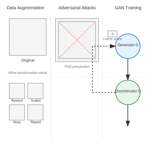
Standard data augmentation applies geometric transformations (e.g., rotation, scaling, translation) and photometric distortions (e.g., brightness, contrast, hue adjustments) to existing images. For a given input image I, a transformed version I' is generated via:
where aij defines affine transformations, (tx, ty) is translation, and ε represents additive noise. Advanced techniques like elastic deformations simulate non-rigid object variations, improving performance in medical imaging applications.
Adversarial Data Augmentation
Adversarial augmentation introduces worst-case perturbations to training data, enhancing model resilience. Given a model fθ with parameters θ, the adversarial example xadv is generated by solving:
where δ is a bounded perturbation within set Δ, and ℒ is the loss function. Projected Gradient Descent (PGD) is commonly used to approximate this optimization:
Training on such adversarially augmented data improves robustness against both natural corruptions and adversarial attacks.
Synthetic Data Generation
When real-world data is scarce or expensive to acquire, synthetic data generation techniques like Generative Adversarial Networks (GANs) or physics-based simulators create photorealistic training samples. For GANs, the generator G and discriminator D are trained via minimax optimization:
Modern variants like StyleGAN3 and Diffusion Models produce high-fidelity images with controllable attributes. In autonomous driving, simulators like CARLA generate diverse driving scenarios with precise ground truth annotations for lidar, segmentation, and depth estimation tasks.
Domain Randomization
Domain randomization bridges the sim-to-real gap by randomizing rendering parameters (e.g., textures, lighting, camera angles) during synthetic data generation. This forces the model to focus on invariant features rather than simulator-specific artifacts. The technique is particularly effective in robotics, where real-world data collection is prohibitively expensive.
Recent work in neural rendering, such as Neural Radiance Fields (NeRFs), enables photorealistic novel view synthesis from sparse input images. By combining NeRF-based data generation with domain randomization, models can be trained on diverse, high-quality synthetic data that closely mimics real-world conditions.
Architectural Choices for Robust Vision Models
Robustness in vision models is heavily influenced by architectural design choices, which determine how well a model generalizes under distribution shifts, adversarial attacks, or noisy inputs. Advanced architectures must balance expressiveness with stability, leveraging inductive biases that align with the structure of visual data while mitigating vulnerabilities.
Residual Connections and Skip Connections
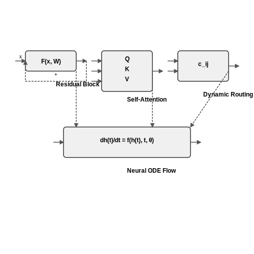
Residual networks (ResNets) introduced skip connections to mitigate vanishing gradients in deep networks. The residual block computes:
where F(x, W) represents the learned transformation, and x is the identity shortcut. This design ensures gradients flow directly through the network, improving training stability and adversarial robustness. Variants like Wide ResNets increase the number of channels per layer, enhancing feature diversity without sacrificing gradient propagation.
Self-Attention and Vision Transformers
Vision Transformers (ViTs) replace convolutional inductive biases with self-attention mechanisms, capturing long-range dependencies critical for robustness. The self-attention operation for an input patch xi is:
where Q, K, V are learned query, key, and value matrices. ViTs exhibit strong out-of-distribution generalization due to their global receptive field, but require large-scale pretraining for optimal robustness. Hybrid architectures like ConvNeXt blend convolutional locality with transformer-like scaling.
Stochastic Depth and Dynamic Routing
Stochastic depth randomly drops layers during training, acting as a regularizer that forces the network to maintain robust feature hierarchies. Dynamic routing mechanisms, as seen in Capsule Networks, learn part-whole relationships through iterative agreement:
where bij are logits updated via routing-by-agreement. These methods improve invariance to spatial transformations but increase computational overhead.
Neural ODEs and Continuous-Depth Models
Neural Ordinary Differential Equations (ODEs) parameterize hidden state evolution as:
solved through adaptive numerical integration. This formulation provides memory efficiency and smooth decision boundaries, reducing sensitivity to input perturbations. However, trade-offs exist in training speed versus robustness guarantees.
Architectural Invariance Inductive Biases
Equivariant networks enforce symmetry constraints through weight sharing patterns. For rotation equivariance in group convolutional networks:
where G is the symmetry group. Such architectures achieve certified robustness against predefined transformations but may lack flexibility for complex real-world variations.
Emerging directions include sparse mixture-of-experts models, which dynamically activate subnetworks based on input, and neural memory-augmented designs that separate feature extraction from robust memory access. The choice of architecture must align with the specific robustness requirements—whether adversarial defense, domain generalization, or noise immunity—while considering computational constraints.
4.3 Post-Training Robustness Enhancements
Post-training robustness enhancements focus on improving model resilience without retraining the underlying architecture. These techniques are particularly valuable when computational resources for full retraining are limited or when deploying pre-trained models in adversarial environments.
Adversarial Fine-Tuning
Adversarial fine-tuning introduces perturbations during the fine-tuning phase to expose the model to worst-case inputs. Given a pre-trained model fθ with parameters θ, the objective function becomes:
where δ represents the adversarial perturbation bounded by ϵ under some norm (typically L∞ or L2). This min-max optimization forces the model to maintain performance under input variations.
Randomized Smoothing
Randomized smoothing constructs a robust classifier g from the base model f by averaging predictions over noise-corrupted inputs:
The method provides certified robustness guarantees against L2 perturbations of size R, where:
with pA and pB being the top two class probabilities, and Φ the standard normal CDF.
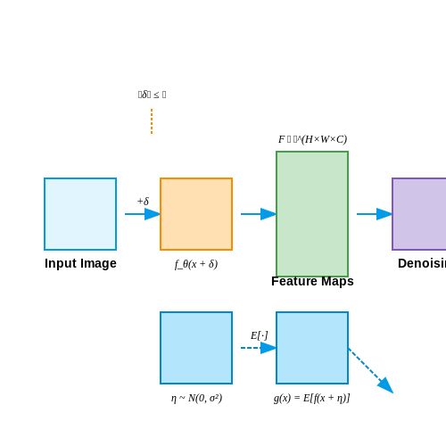
Feature Denoising
Feature denoising modules inserted into pre-trained networks filter adversarial artifacts in intermediate representations. For a feature map F ∈ ℝH×W×C, non-local means denoising computes:
where 𝒞(F) normalizes the weights. This operation preserves semantic content while attenuating high-frequency adversarial patterns.
Gradient Masking Mitigation
Models hardened via gradient masking often exhibit false robustness. Effective post-hoc solutions include:
- Input diversification: Applying random transformations (rotations, crops) before inference
- Stochastic activation pruning: Randomly dropping neurons during forward passes
- Ensemble distillation: Combining predictions from multiple perturbed versions of the model
Certifiable Defenses
Recent advances in convex relaxation provide post-training certification methods. For a neural network with ReLU activations, the robustness verification problem can be formulated as:
where zi represents layer activations and the constraints encode ReLU behavior. Solving this linear program yields guaranteed robustness bounds.
Practical Implementation Considerations
When applying these techniques:
- Measure both clean accuracy and robust accuracy (under PGD, AutoAttack)
- Profile computational overhead - some methods (e.g., randomized smoothing) require 100-1000× more inferences
- Evaluate transferability across threat models (Lp norms, geometric transformations)
- Monitor for gradient obfuscation that may produce false robustness measurements
5. Bias and Fairness in Robust Vision Models
5.1 Bias and Fairness in Robust Vision Models
Bias in vision models arises when a model systematically underperforms for certain demographic groups due to skewed training data or flawed optimization objectives. Fairness, in contrast, requires equitable performance across subgroups, often quantified using statistical parity, equalized odds, or other group-based metrics. The interplay between robustness and fairness is non-trivial: adversarial training, for instance, can exacerbate bias by disproportionately affecting underrepresented classes.
Sources of Bias in Vision Models
Bias can originate from multiple stages of the machine learning pipeline:
- Dataset bias: Training data may underrepresent certain groups or contain stereotypical associations. For example, face recognition datasets historically overrepresented lighter-skinned individuals, leading to higher error rates for darker-skinned faces.
- Labeling bias: Annotators may inject subjective judgments, such as associating certain occupations with specific genders.
- Architectural bias: Model capacity or inductive biases may favor certain feature distributions. Convolutional networks, for instance, prioritize local texture over global shape, which can disadvantage some classes.
Quantifying Fairness
Formally, let Y be the model's predictions, A the sensitive attribute (e.g., gender, race), and Y* the ground truth. Common fairness metrics include:
Violations of these conditions indicate bias. For vision models, these are often measured per-class (e.g., accuracy disparities in object detection across geographic regions).
Bias-Robustness Trade-offs
Adversarial training improves robustness by minimizing the worst-case loss:
However, this can amplify bias. Underrepresented groups may have fewer adversarial examples in the training set, causing the model to over-optimize robustness for majority groups. Empirical studies show that standard adversarial training increases the performance gap between gender subgroups by up to 40% in some face recognition tasks.
Mitigation Strategies
Several approaches jointly optimize for robustness and fairness:
- Fair adversarial training: Modify the adversarial objective to include subgroup-specific perturbations:
- Reweighting: Assign higher loss weights to underrepresented groups during adversarial training.
- Feature disentanglement: Use auxiliary networks to isolate sensitive attributes from robust features.
Case Study: Medical Imaging
In chest X-ray classification, models trained on US hospital data exhibit racial bias—lower sensitivity for Black patients. Adversarial robustness further reduces sensitivity for this group by 12-18% compared to White patients when tested on perturbed images. Mitigation via subgroup-specific adversarial training restores parity while maintaining overall robustness.
5.2 Security Risks and Mitigation Strategies
Vision models, particularly deep neural networks, are vulnerable to adversarial attacks that exploit their decision boundaries. These attacks often involve small, carefully crafted perturbations to input images that are imperceptible to humans but cause misclassification. The vulnerability stems from the high-dimensional, non-linear nature of deep learning models, where slight input variations can lead to disproportionate changes in output.
Types of Adversarial Attacks
Adversarial attacks can be categorized based on the attacker's knowledge and goals:
- White-box attacks: The attacker has full knowledge of the model architecture, parameters, and training data. Common methods include the Fast Gradient Sign Method (FGSM) and Projected Gradient Descent (PGD).
- Black-box attacks: The attacker has no internal knowledge of the model but can query it to observe input-output behavior. Transferability of adversarial examples across models enables these attacks.
- Targeted vs. non-targeted: Targeted attacks aim to misclassify inputs into a specific wrong class, while non-targeted attacks simply cause any incorrect classification.
Mathematical Formulation of Adversarial Examples
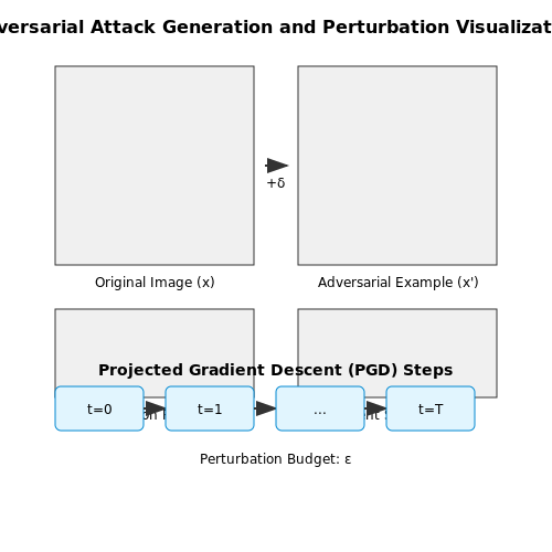
Given a classifier f and input x with true label y, an adversarial example x' satisfies:
where ε is a small perturbation budget and ‖·‖p is typically the L∞ or L2 norm. The FGSM attack generates perturbations as:
where J is the loss function. More sophisticated iterative methods like PGD solve:
where Π projects back to the ε-ball around x and α is the step size.
Defensive Strategies
Adversarial Training
The most empirically robust defense involves training on adversarial examples generated during the learning process. The min-max objective becomes:
where θ represents model parameters. This forces the model to learn more stable decision boundaries.
Input Transformation and Randomization
Preprocessing defenses include:
- Feature squeezing: Reducing color bit depth or spatial smoothing to eliminate adversarial perturbations
- Random resizing/padding: Breaking the spatial structure of adversarial patterns
- Certifiable defenses: Methods like randomized smoothing that provide provable robustness guarantees
Architectural Improvements
Modified network architectures can improve robustness:
- Lipschitz constraints: Limiting the maximum change in output relative to input changes
- Denoising layers: Explicit modules to remove adversarial perturbations
- Attention mechanisms: Focusing on semantically meaningful regions less susceptible to local perturbations
Evaluation Metrics for Robustness
Standard evaluation protocols include:
- Attack success rate: Percentage of adversarial examples that cause misclassification
- Robust accuracy: Accuracy on adversarially perturbed test sets
- Certified radius: Largest perturbation radius for which robustness can be mathematically guaranteed
Recent benchmarks like RobustBench provide standardized evaluations across different threat models and perturbation budgets.
Emerging Threats and Countermeasures
New attack vectors continue to emerge:
- Physical-world attacks: Adversarial patterns that work under varying viewpoints and lighting conditions
- Universal perturbations: Single perturbation pattern that fools a model on most inputs
- Backdoor attacks: Training-time attacks that embed triggers activated by specific input patterns
Defenses against these require combinations of formal verification, anomaly detection, and ensemble methods. Research in certified defenses using convex relaxations or interval bound propagation shows promise for providing mathematical guarantees of robustness.
5.3 Regulatory and Industry Standards for Robust AI
Regulatory frameworks and industry standards play a critical role in ensuring the robustness of vision models, particularly in high-stakes applications such as autonomous vehicles, medical imaging, and surveillance. Compliance with these standards mitigates risks associated with adversarial attacks, distributional shifts, and unintended biases.
Key Regulatory Frameworks
The EU AI Act categorizes AI systems based on risk levels, mandating rigorous robustness testing for high-risk applications. Vision models deployed in critical infrastructure must undergo conformity assessments, including adversarial robustness evaluations under standardized threat models. Similarly, the U.S. NIST AI Risk Management Framework provides guidelines for stress-testing models against perturbations, with specific provisions for computer vision systems.
Industry-Specific Standards
In healthcare, the FDA’s Software as a Medical Device (SaMD) framework requires vision models to demonstrate robustness against noise, occlusions, and domain shifts. For autonomous systems, ISO 21448 (SOTIF) addresses robustness in perception modules by formalizing metrics for failure modes under environmental uncertainties. These standards often reference quantitative robustness benchmarks, such as:
where f is the model, xi are test samples, yi their true labels, and δ denotes bounded adversarial perturbations.
Certification Protocols
Third-party certifications like UL 4600 for autonomous vehicles enforce robustness testing protocols, including:
- Lp-norm bounded attacks (e.g., PGD under L∞ constraints)
- Natural corruption benchmarks (e.g., ImageNet-C)
- Out-of-distribution detection via metrics like AUROC
These tests are often integrated into CI/CD pipelines, with tools like IBM’s Adversarial Robustness Toolbox automating compliance checks.
Ethical and Legal Implications
Standards such as IEEE 7000-2021 extend robustness requirements to ethical dimensions, mandating fairness audits across demographic subgroups. Legal precedents, like liability cases involving misclassified traffic signs, further underscore the need for adherence to these frameworks. For instance, a vision model’s failure mode analysis must document:
where 𝒟edge represents edge-case scenarios and ε is a risk threshold defined by domain-specific regulations.
6. Key Research Papers and Surveys
6.1 Key Research Papers and Surveys
- SpecFormer: Guarding Vision Transformer Robustness via ... - Springer — These datasets are commonly adopted in studies involving the robustness of vision models [33, 37]. CIFAR-10 and CIFAR-100 datasets each comprise 60, 000 images, categorized into 10 classes and 100 classes, respectively. ImageNet encompasses over 1.2 million training images and 50, 000 test images, distributed across 1, 000 classes.
- Establishing and evaluating trustworthy AI: overview and research ... — Ensuring robustness can be done in two principal ways: (1) by restricting potential models to model types shown to be more robust (e.g., multilinear regression is generally more robust than deep learning), or (2) by explicitly evaluating model robustness and incorporating it in the model selection process.
- A Survey on Evaluation of Large Language Models — In Section 6, we summarize the key findings of this paper. We discuss grand future challenges ... For instance, computer vision models leverage static test sets such as ImageNet ... adversarial robustness, and fine-tuning. GLUE-X is a novel attempt to create a unified benchmark aimed at evaluating the robustness of NLP models in OOD scenarios ...
- Review of large vision models and visual prompt engineering — Recently, the Segment Anything Model (SAM) 53 has brought about a new trend in solving downstream tasks. Models with prompt engineering modules can solve a wide range of downstream tasks through prompts. 12, 53, 54 These models' remarkable zero-shot generalization capability highlights the significance of prompt engineering in downstream tasks. 55 However, applying large vision model (LVM) to ...
- A survey of efficient fine-tuning methods for Vision-Language Models ... — Vision Language Model (VLM) is a popular research field located at the fusion of computer vision and natural language processing (NLP). With the emergence of transformer networks and mass web data, numerous large scale VLMs or Vision-Language Pre-training Models (VLPM) have been achieving state-of-the-art results in many tasks, such as retrieval (CLIP) and generation (DALL-E).
- Rain Rendering for Evaluating and Improving Robustness to ... - Springer — Rain fills the atmosphere with water particles, which breaks the common assumption that light travels unaltered from the scene to the camera. While it is well-known that rain affects computer vision algorithms, quantifying its impact is difficult. In this context, we present a rain rendering pipeline that enables the systematic evaluation of common computer vision algorithms to controlled ...
- A Survey of Robustness and Safety of 2D and 3D Deep Learning Models ... — The significant strides of deep learning (DL) algorithms have driven considerable technological progress in computer vision (CV) tasks, which are widely deployed in various safety-critical and mission-critical systems like identity authentication and self-driving vehicles. These applications depend on the assumption that these deep learning models are trustworthy and robust against small ...
- Evaluating the Robustness of Deep Learning Models against ... - MDPI — This study evaluated the generation of adversarial examples and the subsequent robustness of an image classification model. The attacks were performed using the Fast Gradient Sign method, the Projected Gradient Descent method, and the Carlini and Wagner attack to perturb the original images and analyze their impact on the model's classification accuracy. Additionally, image manipulation ...
- A.I. Robustness: a Human-Centered Perspective on Technological ... — One of the core principles of Trustworthy AI is robustness [], defined in Machine Learning (ML) as the insensitivity of a model's performance to miscalculations of its parameters [158, 273].Examples like Tesla's Full Self-Driving mechanism erroneously identifying the moon as a yellow traffic light, 1 or Autopilot being fooled by stickers placed on the ground, 2 show that AI systems might ...
- A comprehensive evaluation framework for deep model robustness — Consequently, conducting rigorous and comprehensive evaluation on model robustness becomes particularly important. To comprehensively evaluate the model robustness for DNNs, a number of works have been proposed. A uniform platform for adversarial robustness analysis named DEEPSEC [8] is proposed to measure the vulnerability of deep learning ...
6.2 Open-Source Tools and Libraries
- Analyzing the Quality Attributes of AI Vision Models in Open ... — The growth of open-source artificial intelligence (AI) models has significant advancements in computer vision technologies (Dosovitskiy et al., 2020; Liu et al., 2022; Wu et al., 2021; Liu et al., 2021; Xie et al., 2021; He et al., 2016).These state-of-the-art models, increasingly accessible in the open community (Wolf et al., 2019) facilitate a wide range of applications across various domains.
- Robin: a Suite of Multi-Scale Vision-Language Models and the CHIRP ... — The advent of powerful foundation models like GPT-4V offers a new way to evaluate weaker models, moving beyond traditional, rigid metrics such as exact string matching, as done in Hudson & Manning (); Mishra et al. (); Singh et al. ().Early evidence from benchmarks like MM-Vet Yu et al. and VQA tasks Agrawal et al. suggests that evaluating with stronger models offers a promising path towards ...
- PDF SAFARI: Versatile and Efficient Evaluations for Robustness of ... — of how robust in general the model is whenever a misin-terpretation can be found (in line with the insight gained from evaluating classification robustness [45]). We intro-duce two metrics concerning the worst-case interpretation discrepancy and a probabilistic metric to calculate the pro-portion of misinterpretations in the local norm-ball around
- Adversarial Robustness Toolbox (ART) - GitHub — 中文README请按此处. Adversarial Robustness Toolbox (ART) is a Python library for Machine Learning Security. ART is hosted by the Linux Foundation AI & Data Foundation (LF AI & Data). ART provides tools that enable developers and researchers to defend and evaluate Machine Learning models and applications against the adversarial threats of Evasion, Poisoning, Extraction, and Inference.
- Welcome to the Adversarial Robustness Toolbox — Welcome to the Adversarial Robustness Toolbox¶. Adversarial Robustness Toolbox (ART) is a Python library for Machine Learning Security. ART provides tools that enable developers and researchers to evaluate, defend, certify and verify Machine Learning models and applications against the adversarial threats of Evasion, Poisoning, Extraction, and Inference.
- RobustCheck: A Python package for black-box robustness assessment of ... — A contributing factor to this oversight is the complexity involved in assessing model robustness. This paper introduces RobustCheck, a Python package designed for evaluating the adversarial robustness of computer vision models. Utilizing black-box adversarial techniques, it allows for the assessment of model resilience without internal model ...
- Top Computer Vision Libraries : OpenCV, TensorFlow, PyTorch — Discover the essential computer vision libraries for your projects. This comprehensive guide covers OpenCV, TensorFlow, PyTorch, scikit-image, Dlib, SimpleCV, Mahotas, OpenFace, Kornia, and YOLO. Learn about installation, key features, and practical examples like image classification, object detection, and face recognition. Compare libraries and choose the best one for your needs while ...
- PDF Towards Robust Vision Transformer - CVF Open Access — ysis, we design a robust vision transformer and introduce two novel techniques to further reduce the fragility of ViT models. 3. Robustness Analysis of Designed Compo-nents We give the robustness analysis of four main components in ViTs: patch embedding, position embedding, transformer blocks and classification head. DeiT-Ti [40] is used as the ...
- A comprehensive evaluation framework for deep model robustness — Consequently, conducting rigorous and comprehensive evaluation on model robustness becomes particularly important. To comprehensively evaluate the model robustness for DNNs, a number of works have been proposed. A uniform platform for adversarial robustness analysis named DEEPSEC [8] is proposed to measure the vulnerability of deep learning ...
- Towards adversarial robustness verification of no-reference image- and ... — Overall, neural-networks-based solutions show state-of-the-art results for a wide range of computer-vision tasks. Despite their remarkable success, neural-network methods have proven to be vulnerable to perturbations of the inputs (Szegedy et al., 2013, Goodfellow et al., 2014).Adversarial attacks became famous for their application to fool object classification and detection methods.
6.3 Recommended Courses and Tutorials
- AVIBench: Towards Evaluating the Robustness of Large Vision-Language ... — In this section, we analyze the relationship between the robustness to AVIs and factors such as model structure, training data, and training methods, using evaluation results from various LVLMs. Despite the differences in LVLMs' structures and training data, the overall framework remains consistent, involving visual encoders, Large Language ...
- PDF Benchmarking Robustness of Adaptation Methods on Pre-trained Vision ... — Benchmarking Robustness of Adaptation Methods on Pre-trained Vision-Language Models (Supplementary) Shuo Chen 1,3∗Jindong Gu 2Zhen Han4 †Yunpu Ma Philip Torr Volker Tresp1 1Institute of Informatics, LMU Munich 2Department of Engineering Science, University of Oxford 3 Siemens AG 4Amazon [email protected], [email protected] 1 ...
- GitHub - MadryLab/robustness: A library for experimenting with ... — For each value of ε-test, we highlight the best robust accuracy achieved over different ε-train in bold. Note #1: We did not perform any hyperparameter tuning and simply used the same hyperparameters as standard training. It is likely that exploring different training hyperparameters will increasse these robust accuracies by a few percent points.
- SpecFormer: Guarding Vision Transformer Robustness via ... - Springer — They evaluate the efficacy of these models in terms of corruption robustness for semantic segmentation and object detection, achieving state-of-the-art results. Additionally, [ 14 ] compared the DeiT [ 49 ], CaiT [ 50 ], and XCiT [ 1 ] ViT variants in adversarial training and discovered that XCiT was the most effective.
- PDF A Large-scale Robustness Analysis of Video Action Recognition Models — tations in model robustness and present a real-world dataset, UCF101-DS, which contains realistic distribution shifts, to further validate some of these findings. We believe this study will serve as a benchmark for future research in robust video action recognition 1. 1. Introduction Robustness of deep learning models against real-world
- PDF Visual Place Recognition: Building an Evaluation Framework for Model ... — works in the eld of GAN models, we generated two long-term corrupted datasets: night time and rainy weather starting from a single ground truth subset of the MSLS validation dataset. [32] 2 PREVIOUS WORK 2.1 Robustness in Visual Place Recognition The need for robust models in VPR is inferred from the applications in which this technology is ...
- PDF SAFARI: Versatile and Efficient Evaluations for Robustness of ... — fied the best training scheme to improve both aspects. In summary, the key contributions of this paper include: •Two diverse metrics, worst-case interpretation discrep-ancy and probabilistic interpretation robustness, com-plement each other as a versatile approach, allowing for a holistic evaluation of interpretation robustness.
- [2105.07926] Towards Robust Vision Transformer — Robustness Benchmarks. The rigorous benchmarks are important for evaluating and understanding the robustness of deep models. Early works focus on the model safety under the adversarial examples with constrained perturbations [11, 38].In real-world applications, the phenomenon of image corruption or out-of-distribution is more commonly appeared.
- A Dynamic Visual Benchmark for Evaluating Mathematical Reasoning ... — We present DynaMath, a curated evaluation dataset aimed at assessing the robustness of visual language models (VLMs) in multimodal mathematical reasoning across a wide variety of mathematical tasks with dynamic visual and textual contexts.Our benchmark consists of 501 seed questions, each represented as a Python program. There are 227 (45.3%) sourced from established visual math datasets ...
- A comprehensive evaluation framework for deep model robustness — Consequently, conducting rigorous and comprehensive evaluation on model robustness becomes particularly important. To comprehensively evaluate the model robustness for DNNs, a number of works have been proposed. A uniform platform for adversarial robustness analysis named DEEPSEC [8] is proposed to measure the vulnerability of deep learning ...